
Use of a Dielectric Sensor for Salinity Determination on an Extensive Green Roof Substrate


Abstract
:1. Introduction
2. Materials and Methods
2.1. Experimental Setup
2.2. Turfgrass Establishment and Irrigation
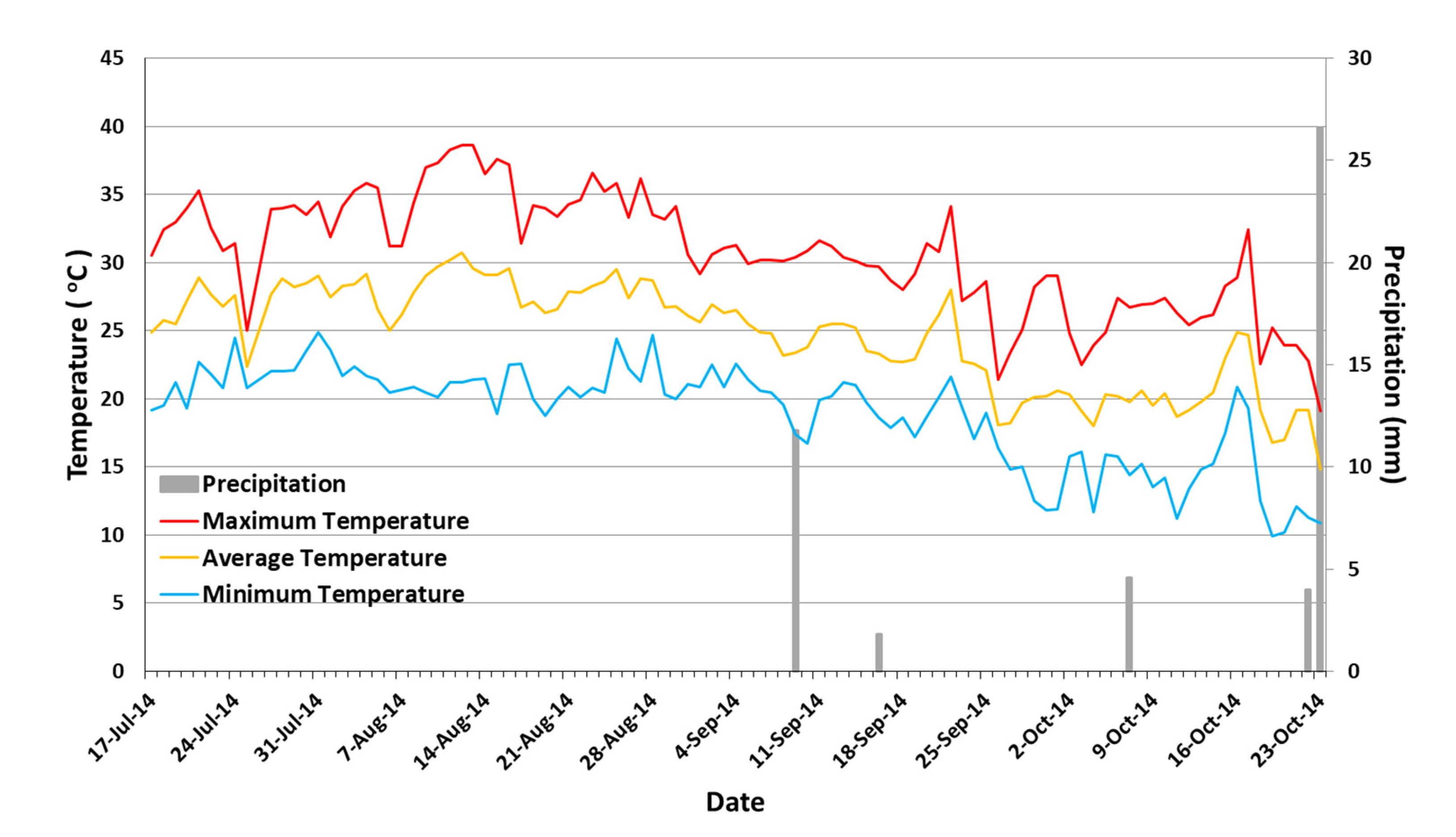
2.3. Meteorological Data
2.4. Measurements
2.5. Experimental Methodology and Statistics
3. Results and Discussion
4. Conclusions
Author Contributions
Funding
Institutional Review Board Statement
Informed Consent Statement
Data Availability Statement
Conflicts of Interest
References
- Cascone, S. Green roof design: State of the art on technology and materials. Sustainability 2019, 11, 3020. [Google Scholar] [CrossRef] [Green Version]
- Forschungsgesellschaft Landschaftsentwicklung Landschaftsbau e.V. (FLL). Guidelines for the Planning, Construction and Maintenance of Green Roofing-Green Roofing Guideline; Forschungsgesellschaft Landschaftsentwicklung Landschaftsbau e.V. (FLL): Bonn, Germany, 2008. [Google Scholar]
- Ntoulas, N.; Nektarios, P.A.; Kapsali, T.-E.; Kaltsidi, M.-P.; Han, L.; Yin, S. Determination of the physical, chemical, and hydraulic characteristics of locally available materials for formulating extensive green roof substrates. HortTechnology 2015, 25, 774–784. [Google Scholar] [CrossRef] [Green Version]
- Eksi, M.; Sevgi, O.; Akburak, S.; Yurtseven, H.; Esin, I. Assessment of recycled or locally available materials as green roof substrates. Ecol. Eng. 2020, 156, 105966. [Google Scholar] [CrossRef]
- Nektarios, P.; Ntoulas, N.; Kotopoulis, G.; Ttoulou, T.; Ilia, P. Festuca arundinacea drought tolerance and evapotranspiration when grown on two extensive green roof substrate depths and under two irrigation regimes. Eur. J. Hortic. Sci. 2014, 79, 142–149. [Google Scholar]
- Graceson, A.; Hare, M.; Hall, N.; Monaghan, J. Use of inorganic substrates and composted green waste in growing media for green roofs. Biosyst. Eng. 2014, 124, 1–7. [Google Scholar] [CrossRef]
- Ntoulas, N.; Nektarios, P.A.; Kotopoulis, G.; Ilia, P.; Ttooulou, T. Quality assessment of three warm-season turfgrasses growing in different substrate depths on shallow green roof systems. Urban For. Urban Green 2017, 26, 163–168. [Google Scholar] [CrossRef]
- Ntoulas, N.; Varsamos, I. Performance of two seashore paspalum (Paspalum vaginatum Sw.) varieties growing in shallow green roof substrate depths and irrigated with seawater. Agronomy 2021, 11, 250. [Google Scholar] [CrossRef]
- Ntoulas, N.; Nektarios, P.A. Paspalum vaginatum NDVI when grown on shallow green roof systems and under moisture deficit conditions. Crop. Sci. 2017, 57, S-147–S-160. [Google Scholar] [CrossRef]
- Xu, C.; Liu, Z.; Cai, G.; Zhan, J. Experimental study on the selection of common adsorption substrates for extensive green roofs (EGRs). Water Sci. Technol. 2021, 83, 961–974. [Google Scholar] [CrossRef]
- Williams, N.S.; Rayner, J.P.; Raynor, K.J. Green roofs for a wide brown land: Opportunities and barriers for rooftop greening in Australia. Urban For. Urban Green 2010, 9, 245–251. [Google Scholar] [CrossRef]
- Dwivedi, A.; Mohan, B.K. Impact of green roof on micro climate to reduce urban heat island. Remote Sens. Appl. Soc. Environ. 2018, 10, 56–69. [Google Scholar] [CrossRef]
- Motlagh, S.H.B.; Pons, O.; Hosseini, S.A. Sustainability model to assess the suitability of green roof alternatives for urban air pollution reduction applied in Tehran. Build. Environ. 2021, 194, 107683. [Google Scholar] [CrossRef]
- Soulis, K.X.; Ntoulas, N.; Nektarios, P.A.; Kargas, G. Runoff reduction from extensive green roofs having different substrate depth and plant cover. Ecol. Eng. 2017, 102, 80–89. [Google Scholar] [CrossRef]
- Akbari, H.; Pomerantz, M.; Taha, H. Cool surfaces and shade trees to reduce energy use and improve air quality in urban areas. Sol. Energy 2001, 70, 295–310. [Google Scholar] [CrossRef]
- Agra, H.; Solodar, A.; Bawab, O.; Levy, S.; Kadas, G.J.; Blaustein, L.; Greenbaum, N. Comparing grey water versus tap water and coal ash versus perlite on growth of two plant species on green roofs. Sci. Total Environ. 2018, 633, 1272–1279. [Google Scholar] [CrossRef]
- Stratigea, D.; Makropoulos, C. Balancing water demand reduction and rainfall runoff minimisation: Modelling green roofs, rainwater harvesting and greywater reuse systems. Water Supply 2015, 15, 248–255. [Google Scholar] [CrossRef]
- Richards, L.A. Diagnosis and Improvement of Saline and Alkali Soils; Agriculture Handbook No. 60; United States Department of Agriculture: Washington, DC, USA, 1954. [Google Scholar]
- Kargas, G.; Popescou, P.; Kaliontzis, N.; Marougas, D.; Kerkides, P. Estimation of the electrical conductivity of saturated paste extract using a dielectric sensor. J. Irrig. Drain. Eng. 2017, 143, 04016086. [Google Scholar] [CrossRef]
- Rhoades, J.; Raats, P.; Prather, R. Effects of liquid-phase electrical conductivity, water content, and surface conductivity on bulk soil electrical conductivity. Soil Sci. Soc. Am. J. 1976, 40, 651–655. [Google Scholar] [CrossRef]
- Malicki, M.; Walczak, R. Evaluating soil salinity status from bulk electrical conductivity and permittivity. Eur. J. Soil Sci. 1999, 50, 505–514. [Google Scholar] [CrossRef]
- Hilhorst, M.A. A pore water conductivity sensor. Soil Sci. Soc. Am. J. 2000, 64, 1922–1925. [Google Scholar] [CrossRef] [Green Version]
- Kargas, G.; Kerkides, P. Evaluation of a dielectric sensor for measurement of soil-water electrical conductivity. J. Irrig. Drain. Eng. 2010, 136, 553–558. [Google Scholar] [CrossRef]
- Kargas, G.; Kerkides, P. Comparison of two models in predicting pore water electrical conductivity in different porous media. Geoderma 2012, 189–190, 563–573. [Google Scholar] [CrossRef]
- Kargas, G.; Persson, M.; Kanelis, G.; Markopoulou, I.; Kerkides, P. Prediction of soil solution electrical conductivity by the permittivity corrected linear model using a dielectric sensor. J. Irrig. Drain. Eng. 2017, 143, 04017030. [Google Scholar] [CrossRef]
- Wilczek, A.; Szypłowska, A.; Skierucha, W.; Cieśla, J.; Pichler, V.; Janik, G. Determination of soil pore water salinity using an FDR sensor working at various frequencies up to 500 MHz. Sensors 2012, 12, 10890–10905. [Google Scholar] [CrossRef]
- Regalado, C.M.; Ritter, A.; Rodríguez-González, R.M. Performance of the commercial WET capacitance sensor as compared with Time Domain Reflectometry in volcanic soils. Vadose Zone J. 2007, 6, 244–254. [Google Scholar] [CrossRef]
- Bañón, S.; Álvarez, S.; Bañón, D.; Ortuño, M.F.; Sánchez-Blanco, M.J. Assessment of soil salinity indexes using electrical conductivity sensors. Sci. Hortic. 2001, 285, 110171. [Google Scholar] [CrossRef]
- Kargas, G.; Kerkides, P. Determination of soil salinity based on WET measurements using the concept of salinity index. J. Plant Nutr. Soil Sci. 2018, 181, 600–605. [Google Scholar] [CrossRef]
- Lee, G.; Carrow, R.N.; Duncan, R.R. Growth and water relation responses to salinity stress in halophytic seashore paspalum ecotypes. Sci. Hortic. 2005, 104, 221–236. [Google Scholar] [CrossRef]
- Delta-T Devices. User Manual for the WET Sensor Type WET-2, Version 1.3; Delta-T Devices: Burwell/Cambridge, UK, 2005. [Google Scholar]
- Liu, H.; Todd, J.L.; Luo, H. Turfgrass Salinity Stress and Tolerance—A Review. Plants 2023, 12, 925. [Google Scholar] [CrossRef] [PubMed]
- Pessarakli, M. Screening various cultivars of seashore paspalum (Paspalum vaginatum Swartz) for salt tolerance for potential use as a cover plant in combatting desertification. Int. J. Water Res. Arid Environ. 2018, 7, 36–43. [Google Scholar]
- Kargas, G.; Kerkides, P.; Seyfried, M.S. Response of three soil water sensors to variable solution electrical conductivity in different soils. Vadose Zone J. 2014, 13, vzj2013.09.0169. [Google Scholar] [CrossRef]
- Incrocci, L.; Incrocci, G.; Pardossi, A.; Lock, G.; Nicholl, C.; Balendonck, J. The calibration of wet-sensor for volumetric water content and pore water electrical conductivity in different horticultural substrates. Acta Hortic. 2009, 807, 289–294. [Google Scholar] [CrossRef] [Green Version]


| Parameter | Value (±SE) | Mechanical Analysis | |
|---|---|---|---|
| Particle Size | Percent Retained | ||
| mm | % (w/w) | ||
| pH (CaCl2) | 7.2 (±0.02) | 9.5–6.3 | 1.9 |
| Electrical conductivity, dS m−1 (water, 1:10, m:v) | 0.60 (±0.02) | 6.3–3.2 | 23.6 |
| Dry bulk density, kg L−1 | 0.80 (±0.02) | 3.2–2.0 | 17.3 |
| Saturated bulk density, kg L−1 | 1.30 (±0.05) | 2.0–1.0 | 25.9 |
| Bulk density at maximum field capacity, kg L−1 | 1.20 (±0.03) | 1.0–0.25 | 20.4 |
| Maximum water holding capacity, % (v/v) | 54.2 (±1.65) | 0.25–0.05 | 4.4 |
| Total pore volume, % | 63.8 (±2.30) | 0.05–0.002 | 5.4 |
| Hydraulic conductivity, mm·min−1 | 7.62 (±0.67) | <0.002 | 1.1 |
| Plant available water, % (v/v) | 7.8 (±0.30) | ||
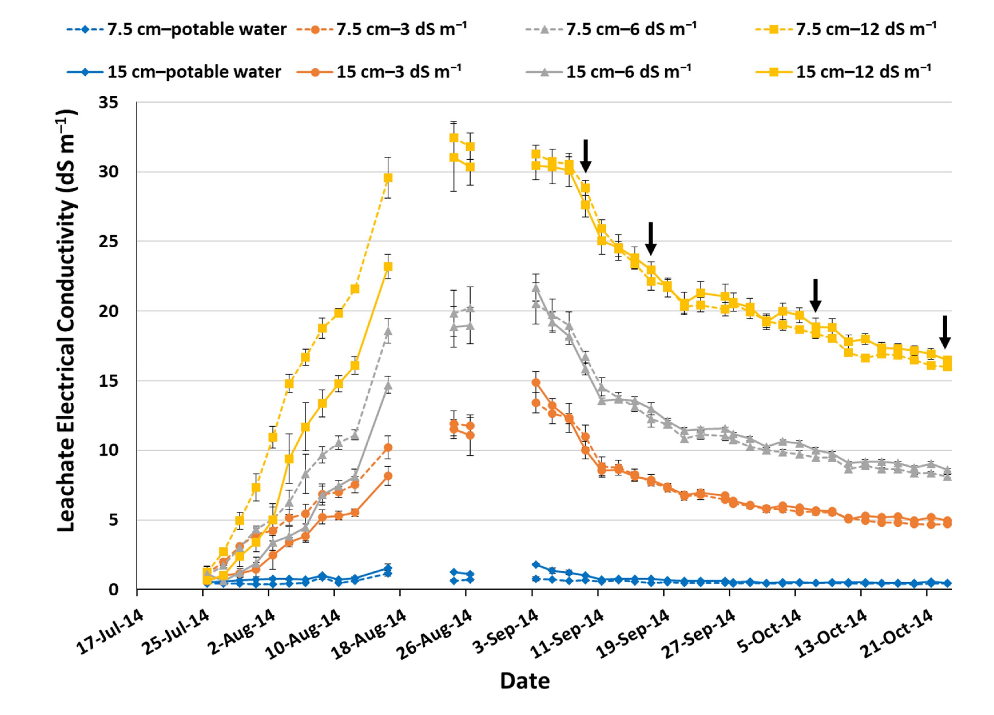
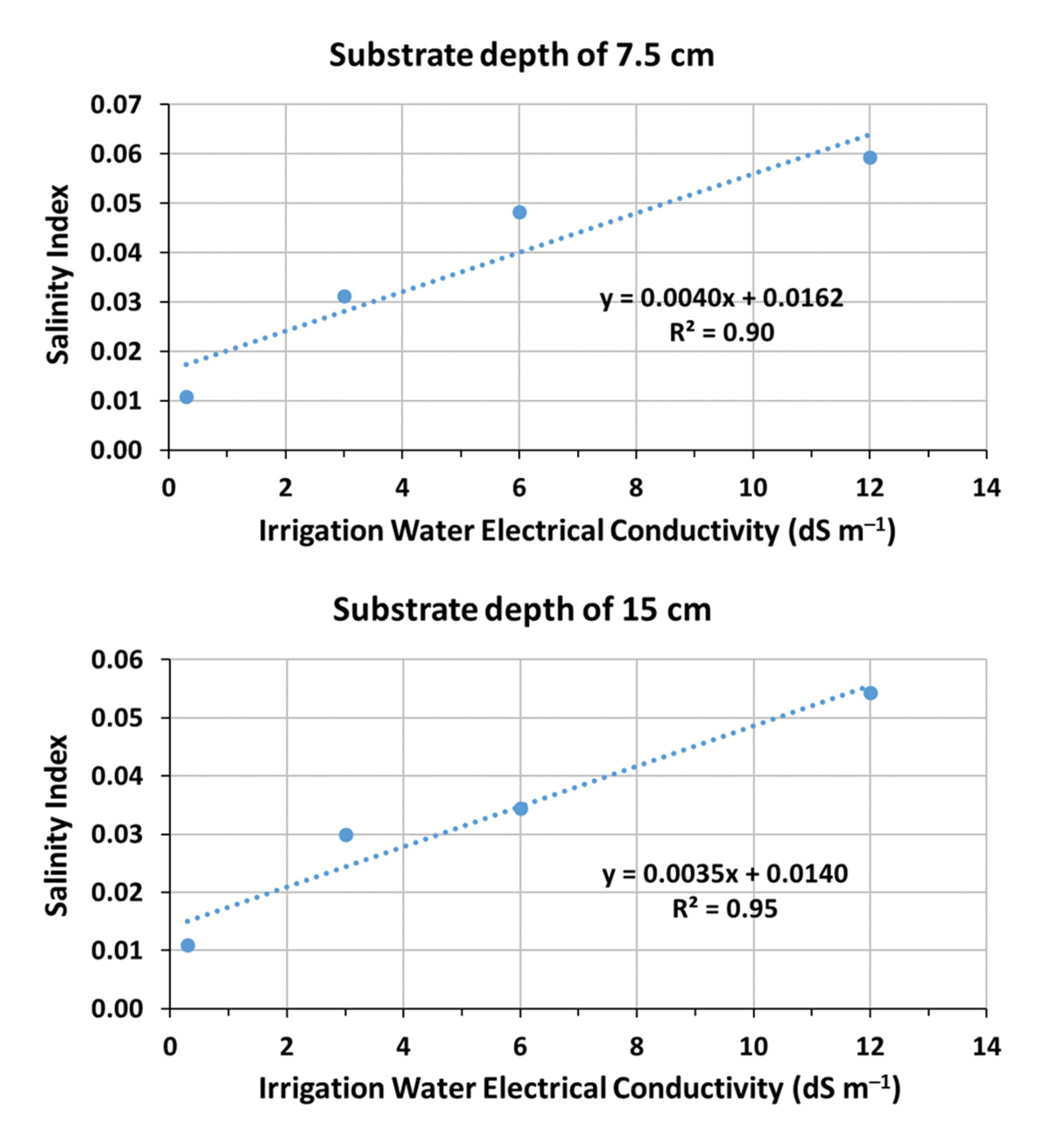
| Irrigation Water Electrical Conductivity (dS m−1) | Salinity Index | Regression Slope between Salinity Index and Irrigation Water Electrical Conductivity | Estimated Mean Substrate Electrical Conductivity (dS m−1) | Measured Mean Leachate Electrical Conductivity (dS m−1) | Relative Error (%) |
|---|---|---|---|---|---|
| Substrate depth of 7.5 cm | |||||
| 0.3 | 0.0109 | 0.0040 | 2.73 | 0.53 | 415.1 |
| 3 | 0.0312 | 0.0040 | 7.80 | 6.86 | 13.7 |
| 6 | 0.0483 | 0.0040 | 12.08 | 11.14 | 8.4 |
| 12 | 0.0593 | 0.0040 | 14.83 | 19.73 | −24.8 |
| Substrate depth of 15 cm | |||||
| 0.3 | 0.0109 | 0.0035 | 3.11 | 0.78 | 298.7 |
| 3 | 0.0300 | 0.0035 | 8.57 | 7.51 | 14.1 |
| 6 | 0.0344 | 0.0035 | 9.83 | 10.54 | −6.7 |
| 12 | 0.0544 | 0.0035 | 15.54 | 18.56 | −16.3 |
Disclaimer/Publisher’s Note: The statements, opinions and data contained in all publications are solely those of the individual author(s) and contributor(s) and not of MDPI and/or the editor(s). MDPI and/or the editor(s) disclaim responsibility for any injury to people or property resulting from any ideas, methods, instructions or products referred to in the content. |
© 2023 by the authors. Licensee MDPI, Basel, Switzerland. This article is an open access article distributed under the terms and conditions of the Creative Commons Attribution (CC BY) license (https://creativecommons.org/licenses/by/4.0/).
Share and Cite
Kargas, G.; Ntoulas, N.; Tsapatsouli, A. Use of a Dielectric Sensor for Salinity Determination on an Extensive Green Roof Substrate. Sensors 2023, 23, 5802. https://doi.org/10.3390/s23135802
Kargas G, Ntoulas N, Tsapatsouli A. Use of a Dielectric Sensor for Salinity Determination on an Extensive Green Roof Substrate. Sensors. 2023; 23(13):5802. https://doi.org/10.3390/s23135802
Chicago/Turabian StyleKargas, Georgios, Nikolaos Ntoulas, and Andreas Tsapatsouli. 2023. "Use of a Dielectric Sensor for Salinity Determination on an Extensive Green Roof Substrate" Sensors 23, no. 13: 5802. https://doi.org/10.3390/s23135802
APA StyleKargas, G., Ntoulas, N., & Tsapatsouli, A. (2023). Use of a Dielectric Sensor for Salinity Determination on an Extensive Green Roof Substrate. Sensors, 23(13), 5802. https://doi.org/10.3390/s23135802