

Wavelet-Based Output-Only Damage Detection of Composite Structures

Abstract
:1. Introduction
2. Modal Identification
- CWT on the recorded response signals is carried out using analytical Morlet function and storing complex-valued CWT coefficients in a matrix form:where is the vector of scale factors, is the vector of translation parameters, and is the signal length.
- Wavelet ridges (in terms of scale parameters ) of each response signal are found by, firstly, finding the and parameters (denoted by and ) corresponding to the maximum value of modulus of CWT coefficients and, secondly, testing the ridge condition at a fixed parameter (time instant when vibration amplitude is maximum).
- Damped natural frequencies are calculated from the derivative of phase between the real and imaginary parts of CWT coefficients along the wavelet ridge line with respect to time. The wavelet ridge line is defined at the ridge scales along the whole time span of free vibrations starting from the time instant .
3. Damage Detection Algorithm
3.1. Phase I—Signal Collection
3.2. Phase II—Feature Extraction
3.3. Phase III—Statistical Control
- Perform a cross-validation partition on the data to create 10 folds where one fold is used for testing and 9 folds are for training. Perform 10 iterations of such a partition, where a different fold is used for testing in each iteration.
- Define a range of bandwidth parameters to test.
- In each training fold and the single testing fold, compute the KDE according to Equation (8) for each value of the bandwidth parameter. Then, compute an error between the KDEs of the testing and each training set according towhere is the number of folds.
- Calculate the cross-validation error as a mean-squared-error of the errors in Equation (9) across all folds for each value according to
- Find the optimum bandwidth parameter by calculating the minimum of these cross-validation errors across all bandwidth values
- 6.
- Consider all available structures of the same type at their reference state.
- 7.
- Perform a modal parameters estimation to form feature vectors and calculate their centroid values for each structure.
- 8.
- Calculate the Euclidean distance between centroid values in all possible combinations of structure pairs.
- 9.
- Calculate the median value of these Euclidean distances and confidence bounds as
4. Experimental Campaign
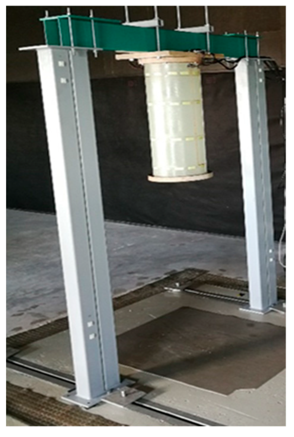
4.1. Specimens
- Item 1—composite cylinder made of fiberglass and epoxy resin;
- Items 2 and 3 —top and bottom annular flanges for cylinder fixation made of laminated plywood (30 mm thickness), respectively;
- Item 4—a network of 48 piezoelectric strain sensors;
- Item 5—wires connecting the sensors;
- Item 6—4 D-SUB type connectors at the places for connector fastening.
4.2. Measurement Subsystem
4.3. Modal Testing
4.4. Test Cases
5. Results
5.1. Time-Frequency Analysis
5.2. Modal Parameter Estimation
5.2.1. Resonant Frequencies
5.2.2. Damping Ratio
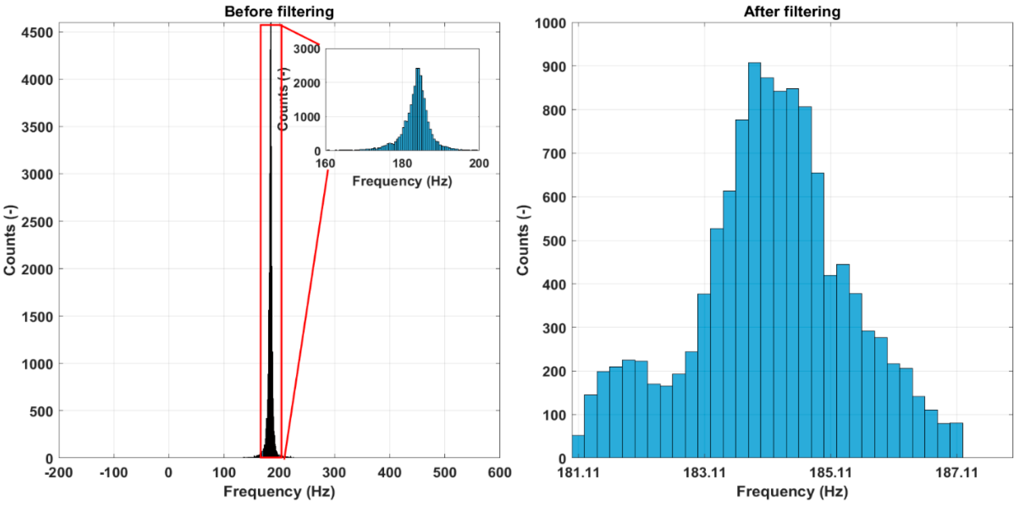
5.2.3. Frequency Filtering
5.3. Kernel Smoothing
5.4. Damage Detection
5.4.1. Threshold Estimation
5.4.2. Damage Indication
5.4.3. Comparison with Mahalanobis Distance
6. Conclusions
- The Euclidean distance of the centroids of the modal features KDEs between the reference and damage states can be used to detect damage.
- The damage indicator proposed shows an upward trend for damage progression, meaning that it is effective in detecting increasing severities of damage.
- Some vibration modes are more sensitive to damage than others. Therefore, multiple vibration modes have to be identified in order to increase the reliability of the damage detection. For example, features originating from the vibration modes at 106 and 176 Hz have significantly higher deviations from the reference than the vibration mode at 185 Hz. Therefore, these vibration modes were more effective in damage detection. On the other hand, these vibration modes could not be identified for all damage cases, while the vibration mode at 185 Hz was present in all scenarios.
- There is a significant scatter of the feature value deviations from reference among the test samples. For the most part, this is due to inconsistencies in the sample design and instrumentation, as mentioned in Section 4.1. Specimens.
- The damage indicator proposed was compared to the Mahalanobis distance metric for damage detection. Both methods yield comparable damage detection accuracy. Therefore, there is no reason to use a more computationally costly Mahalanobis distance approach.
Author Contributions
Funding
Institutional Review Board Statement
Acknowledgments
Conflicts of Interest
References
- Qing, X.P.; Beard, S.J.; Kumar, A.; Ooi, T.K.; Chang, F.-K. Built-in Sensor Network for Structural Health Monitoring of Composite Structure. J. Intell. Mater. Syst. Struct. 2017, 18, 39–49. [Google Scholar] [CrossRef]
- Liu, D.; Luo, M.; Zhang, Z.; Hu, Y.; Zhang, D. Operational modal analysis based dynamic parameters identification in milling of thin-walled workpiece. Mech. Syst. Signal Process 2022, 167, 108469. [Google Scholar] [CrossRef]
- Janeliukstis, R.; Mironovs, D.; Safonovs, A. Statistical Structural Integrity Control of Composite Structures Based on an Automatic Operational Modal Analysis—A Review. Polym. Mech. 2022, 58, 181–208. [Google Scholar] [CrossRef]
- Reynders, E.; De Roeck, G. Reference-based combined deterministic–stochastic subspace identification for experimental and operational modal analysis. Mech. Syst. Signal Process 2008, 22, 617–637. [Google Scholar] [CrossRef]
- Guillaume, P.; Verboven, P.; Vanlanduit, S.; Van Der Auweraer, H.; Peeters, B. A polyreference implementation of the least-squares complex frequency domain-estimator. In Proceedings of the of the IMAC XXI, International Modal Analysis Conference, Kissimmee, FL, USA, 3–6 February 2003. [Google Scholar]
- Zhu, Q.; Wang, Y.; Shen, G. Research and Comparison of Time-frequency Techniques for Nonstationary Signals. J. Comput. 2012, 7, 954–958. [Google Scholar] [CrossRef] [Green Version]
- Hamtaei, M.R.; Anvar, S.A. Estimation of modal parameters of buildings by wavelet transform. In Proceedings of the the 14th World Conference on Earthquake Engineering 14 WCEE, Beijing, China, 12–17 October 2008. [Google Scholar]
- Staszewski, W.J. Identification of Damping in Mdof Systems Using Time-Scale Decomposition. J. Sound Vib. 1997, 203, 283–305. [Google Scholar] [CrossRef]
- Zhang, M.; Huang, X.; Li, Y.; Sun, H.; Zhang, J.; Huang, B. Improved Continuous Wavelet Transform for Modal Parameter Identification of Long-Span Bridges. Shock. Vib. 2020, 2020, 4360184. [Google Scholar] [CrossRef]
- Su, W.C.; Huang, C.S.; Chen, C.H.; Liu, C.Y.; Huang, H.C.; Le, Q.T. Identifying the Modal Parameters of a Structure from Ambient Vibration Data via the Stationary Wavelet Packet. Comput. Civ. Infrastruct. Eng. 2014, 29, 738–757. [Google Scholar] [CrossRef]
- Wei, P.; Li, Q.; Sun, M.; Huang, J. Modal identification of high-rise buildings by combined scheme of improved empirical wavelet transform and Hilbert transform techniques. J. Build. Eng. 2023, 63, 105443. [Google Scholar] [CrossRef]
- Sun, H.; Di, S.; Du, Z.; Wang, L.; Xiang, C. Application of multisynchrosqueezing transform for structural modal parameter identification. J. Civ. Struct. Health Monit. 2021, 11, 1175–1188. [Google Scholar] [CrossRef]
- Nagarajaiah, S.; Basu, B.; Yang, Y. Output-only modal identification and structural damage detection using time–frequency and wavelet techniques for assessing and monitoring civil infrastructures. Sensor Technologies for Civil Infrastructures. In Volume 1: Sensing Hardware and Data Collection Methods for Performance Assessment, 2nd ed.; Woodhead Publishing Series in Civil and Structural Engineering; Woodhead Publishing: Sawston, UK, 2022; pp. 481–529. [Google Scholar]
- Janeliukstis, R. Continuous wavelet transform-based method for enhancing estimation of wind turbine blade natural fre-quencies and damping for machine learning purposes. Measurement 2021, 172, 108897. [Google Scholar] [CrossRef]
- Zimek, A.; Schubert, E. Outlier Detection. In Encyclopedia of Database Systems; Liu, L., Özsu, M., Eds.; Springer: New York, NY, USA, 2017. [Google Scholar]
- Helbing, G.; Ritter, M. Deep Learning for fault detection in wind turbines. Renew. Sustain. Energy Rev. 2018, 98, 189–198. [Google Scholar] [CrossRef]
- Bangalore, P.; Patriksson, M. Analysis of SCADA data for early fault detection, with application to the maintenance management of wind turbines. Renew. Energy 2018, 115, 521–532. [Google Scholar] [CrossRef]
- García, D.; Tcherniak, D.; Trendafilova, I. Damage assessment for wind turbine blades based on a multivariate statistical approach. J. Phys. Conf. Ser. 2015, 628, 12086. [Google Scholar] [CrossRef]
- Movsessian, A.; Cava, D.G.; Tcherniak, D. An artificial neural network methodology for damage detection: Demonstration on an operating wind turbine blade. Mech. Syst. Signal Process. 2021, 159, 107766. [Google Scholar] [CrossRef]
- Sarmadi, H.; Yuen, K. Early damage detection by an innovative unsupervised learning method based on kernel null space and peak-over-threshold. Comput. Civ. Infrastruct. Eng. 2021, 36, 1150–1167. [Google Scholar] [CrossRef]
- Mironov, A.; Mironovs, D. Modal passport of dynamically loaded structures: Application to composite blades. In Proceedings of the 13th International Conference Modern Building Materials, Structures and Techniques, Vilnius, Lithuania, 16–17 May 2019. [Google Scholar] [CrossRef]
- Mironov, A.; Doronkin, P. The Demonstrator of Structural Health Monitoring System of Helicopter Composite Blades. In Proceedings of the ICSI 2021 The 4th International Conference on Structural Integrity, Procedia Structural Integrity 37, Online, 30 August–2 September 2022. [Google Scholar]
- Yang, G.; Yang, Z.-B.; Zhu, M.-F.; Tian, S.-H.; Chen, X.-F. Directional wavelet modal curvature method for damage detection in plates. J. Phys. Conf. Ser. 2022, 2184, 12027. [Google Scholar] [CrossRef]
- Dziedziech, K.; Staszewski, W.J.; Mendrok, K.; Basu, B. Wavelet-Based Transmissibility for Structural Damage Detection. Materials 2022, 15, 2722. [Google Scholar] [CrossRef]
- Colone, L.; Hovgaard, M.; Glavind, L.; Brincker, R. Mass detection, localization and estimation for wind turbine blades based on statistical pattern recognition. Mech. Syst. Signal Process. 2018, 107, 266–277. [Google Scholar] [CrossRef]
- Yang, C.; Zhang, S.; Liu, Y.; Yu, K. Damage detection of bridges under changing environmental temperature using the characteristics of the narrow dimension (CND) of damage features. Measurement 2022, 189, 110640. [Google Scholar] [CrossRef]
- Luo, J.; Huang, M.; Lei, Y. Temperature Effect on Vibration Properties and Vibration-Based Damage Identification of Bridge Structures: A Literature Review. Buildings 2022, 12, 1209. [Google Scholar] [CrossRef]
- Shan, W.; Wang, X.; Jiao, Y. Modeling of Temperature Effect on Modal Frequency of Concrete Beam Based on Field Monitoring Data. Shock. Vib. 2018, 2018, 8072843. [Google Scholar] [CrossRef] [Green Version]


| Specimen | 1 | 2 | 3 | 4 | 5 | |
|---|---|---|---|---|---|---|
| Ridge # | Scale s (-) | f (Hz) | f (Hz) | f (Hz) | f (Hz) | f (Hz) |
| 1 | 5 | 198.6 | - | - | 198.6 | - |
| 2 | 6 | 185.3 | 185.3 | 185.3 | 185.3 | 185.3 |
| 3 | 7 | 172.9 | - | 172.9 | 172.9 | 172.9 |
| 4 | 14 | 106.4 | 106.4 | 106.4 | 106.4 | 106.4 |
| Specimen No. | 1 | 1 | 2 | 2 | 3 | 3 | 4 | 4 | 5 | 5 |
|---|---|---|---|---|---|---|---|---|---|---|
| Filtering | No | Yes | No | Yes | No | Yes | No | Yes | No | Yes |
| Mean (Hz) | 187.38 | 186.49 | 183.58 | 184.15 | 178.41 | 180.03 | 182.38 | 182.21 | 142.70 | 180.77 |
| Variance (Hz2) | 359.10 | 4.97 | 99.40 | 1.54 | 421.48 | 0.94 | 364.81 | 5.29 | 1474.56 | 1.49 |
| Range (Hz) | 1512.70 | 11.48 | 701.68 | 6.08 | 2501.22 | 4.37 | 2061.54 | 10.86 | 872.45 | 6.02 |
| Vibration Mode | Scale 14 (106 Hz) | Scale 7 (176 Hz) | Scale 6 (185 Hz) |
|---|---|---|---|
| 1.432 | 0.871 | 2.863 | |
| CB_lower | 0.614 | 0.289 | 1.455 |
| CB_upper | 3.464 | 2.34 | 4.274 |
Disclaimer/Publisher’s Note: The statements, opinions and data contained in all publications are solely those of the individual author(s) and contributor(s) and not of MDPI and/or the editor(s). MDPI and/or the editor(s) disclaim responsibility for any injury to people or property resulting from any ideas, methods, instructions or products referred to in the content. |
© 2023 by the authors. Licensee MDPI, Basel, Switzerland. This article is an open access article distributed under the terms and conditions of the Creative Commons Attribution (CC BY) license (https://creativecommons.org/licenses/by/4.0/).
Share and Cite
Janeliukstis, R.; Mironovs, D. Wavelet-Based Output-Only Damage Detection of Composite Structures. Sensors 2023, 23, 6121. https://doi.org/10.3390/s23136121
Janeliukstis R, Mironovs D. Wavelet-Based Output-Only Damage Detection of Composite Structures. Sensors. 2023; 23(13):6121. https://doi.org/10.3390/s23136121
Chicago/Turabian StyleJaneliukstis, Rims, and Deniss Mironovs. 2023. "Wavelet-Based Output-Only Damage Detection of Composite Structures" Sensors 23, no. 13: 6121. https://doi.org/10.3390/s23136121