
Bridge Damage Identification Using Deep Neural Networks on Time–Frequency Signals Representation


Abstract
:1. Introduction
2. Related Works
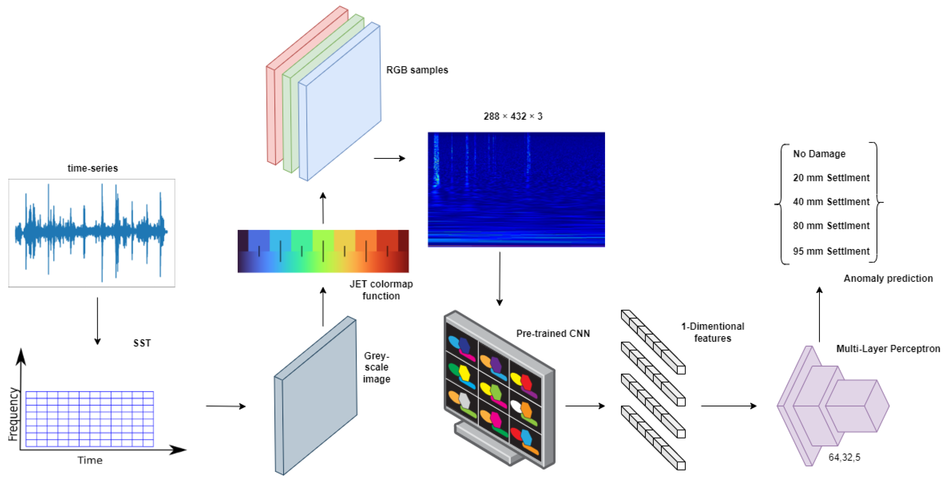
3. Proposed Methods
3.1. Data Pre-Processing
3.2. Feature Extraction and Classification
3.3. Image-Splitting
3.4. Signal-Splitting
4. Implementation Details
4.1. Dataset
- A long-term continuous monitoring test for the year prior to the harm. The purpose of this test was to look at the effects of the environment on the dynamics of the bridge structure.
- A month before the bridge was destroyed, short-term progressive damage testing under various damage scenarios.
4.2. Ambient Vibration Test vs. Forced Vibration Test
4.3. Task and Dataset Definition: The Lowering of Pier Task
4.4. Hyperparameters
4.5. Performance Metrics
5. Results
6. Conclusions
Author Contributions
Funding
Institutional Review Board Statement
Data Availability Statement
Conflicts of Interest
Abbreviations
| SHM | Structural health monitoring |
| SST | Synchrosqueezing transform |
| SDD | System damage detection |
| ML | Machine learning |
| CNN | Convolutional neural networks |
| ANN | Artificial neural networks |
| TF | Time–frequency |
| STFT | Short-time Fourier transform |
| WT | Wavelet transform |
| CWT | Continuous wavelet transform |
| VDD | Vibration-based damage detection |
| AR | Auto-regressive |
| ARMA | Auto-regressive moving-average |
| ARX | Auto-regressive exogenous input |
| CCWT | Continuous Cauchy wavelet transform |
| DL | Deep learning |
| FCN | Fully convolutional networks |
| RNN | Recurrent neural networks |
| Re LU | Rectified linear unit |
| GPU | Graphics processing unit |
| LSTM | Long short-term memory |
| RGB | Red, green and blue |
| EMPA | Swiss Federal Laboratories for Materials Testing |
| FFT | Fast Fourier transform |
| TDNN | Time-delay neural network |
| MLP | Multi-layer perceptron |
References
- Rytter, A. Vibrational Based Inspection of Civil Engineering Structures. Ph.D. Thesis, Aalborg University, Aalborg, Denmark, 1993. [Google Scholar]
- Farrar, C.; Sohn, H.; Hemez, F.; Anderson, M.; Bement, M.; Cornwell, P.; Doebling, S.; Schultze, J.; Lieven, N.; Robertson, A. Damage Prognosis: Current Status and Future Needs; Technical Report, LA-14051-MS; Los Alamos National Laboratory: Los Alamos, NM, USA, 2003. [Google Scholar]
- Inman, D.J.; Farrar, C.R.; Junior, V.L.; Junior, V.S. Damage Prognosis: For Aerospace, Civil and Mechanical Systems; John Wiley & Sons: Hoboken, NJ, USA, 2005. [Google Scholar]
- Cawley, P. Structural health monitoring: Closing the gap between research and industrial deployment. Struct. Health Monit. 2018, 17, 1225–1244. [Google Scholar] [CrossRef] [Green Version]
- Fritzen, C.P. Vibration-Based Methods for SHM; NATO: Geilenkirchen, Germany, 2014. [Google Scholar]
- Choi, S.; Stubbs, N. Damage identification in structures using the time-domain response. J. Sound Vib. 2004, 275, 577–590. [Google Scholar] [CrossRef]
- Cattarius, J.; Inman, D. Time domain analysis for damage detection in smart structures. Mech. Syst. Signal Process. 1997, 11, 409–423. [Google Scholar] [CrossRef]
- Barthorpe, R.J.; Worden, K. Emerging trends in optimal structural health monitoring system design: From sensor placement to system evaluation. J. Sens. Actuator Netw. 2020, 9, 31. [Google Scholar] [CrossRef]
- Banks, H.; Inman, D.; Leo, D.; Wang, Y. An experimentally validated damage detection theory in smart structures. J. Sound Vib. 1996, 191, 859–880. [Google Scholar] [CrossRef]
- Lee, Y.S.; Chung, M.J. A study on crack detection using eigenfrequency test data. Comput. Struct. 2000, 77, 327–342. [Google Scholar] [CrossRef]
- Zhang, Z.; Zhan, C.; Shankar, K.; Morozov, E.V.; Singh, H.K.; Ray, T. Sensitivity analysis of inverse algorithms for damage detection in composites. Compos. Struct. 2017, 176, 844–859. [Google Scholar] [CrossRef]
- Pai, P.F.; Huang, L.; Hu, J.; Langewisch, D.R. Time-frequency method for nonlinear system identification and damage detection. Struct. Health Monit. 2008, 7, 103–127. [Google Scholar] [CrossRef]
- Daubechies, I. The wavelet transform, time-frequency localization and signal analysis. IEEE Trans. Inf. Theory 1990, 36, 961–1005. [Google Scholar] [CrossRef] [Green Version]
- Andria, G.; D’ambrosio, E.; Savino, M.; Trotta, A. Application of Wigner-Ville distribution to measurements on transient signals. In Proceedings of the 1993 IEEE Instrumentation and Measurement Technology Conference, Irvine, CA, USA, 18–20 May 1993; pp. 612–617. [Google Scholar]
- Karami-Mohammadi, R.; Mirtaheri, M.; Salkhordeh, M.; Hariri-Ardebili, M.A. Vibration anatomy and damage detection in power transmission towers with limited sensors. Sensors 2020, 20, 1731. [Google Scholar] [CrossRef] [Green Version]
- Allen, J.B.; Rabiner, L.R. A unified approach to short-time Fourier analysis and synthesis. Proc. IEEE 1977, 65, 1558–1564. [Google Scholar] [CrossRef]
- Yang, Y.; Zhang, Y.; Tan, X. Review on vibration-based structural health monitoring techniques and technical codes. Symmetry 2021, 13, 1998. [Google Scholar] [CrossRef]
- Li, D. Sensor Placement Methods and Evaluation Criteria in Structural Health Monitoring. Ph.D. Thesis, Universoty Siegen, Siegen, Germany, 2012. [Google Scholar]
- Wang, Z.; Yang, J.P.; Shi, K.; Xu, H.; Qiu, F.; Yang, Y. Recent advances in researches on vehicle scanning method for bridges. Int. J. Struct. Stab. Dyn. 2022, 22, 2230005. [Google Scholar] [CrossRef]
- Mousa, M.A.; Yussof, M.M.; Udi, U.J.; Nazri, F.M.; Kamarudin, M.K.; Parke, G.A.; Assi, L.N.; Ghahari, S.A. Application of digital image correlation in structural health monitoring of bridge infrastructures: A review. Infrastructures 2021, 6, 176. [Google Scholar] [CrossRef]
- Yeung, W.; Smith, J. Damage detection in bridges using neural networks for pattern recognition of vibration signatures. Eng. Struct. 2005, 27, 685–698. [Google Scholar] [CrossRef]
- Yan, Y.; Cheng, L.; Wu, Z.; Yam, L. Development in vibration-based structural damage detection technique. Mech. Syst. Signal Process. 2007, 21, 2198–2211. [Google Scholar] [CrossRef]
- Neild, S.; McFadden, P.; Williams, M. A review of time-frequency methods for structural vibration analysis. Eng. Struct. 2003, 25, 713–728. [Google Scholar] [CrossRef]
- Pan, H.; Azimi, M.; Yan, F.; Lin, Z. Time-frequency-based data-driven structural diagnosis and damage detection for cable-stayed bridges. J. Bridge Eng. 2018, 23, 04018033. [Google Scholar] [CrossRef]
- Auger, F.; Flandrin, P.; Lin, Y.; McLaughlin, S.; Meignen, S.; Oberlin, T.; Wu, H.T. Recent advances in time-frequency reassignment and synchrosqueezing. IEEE Trans. Signal Process. 2013, 30, 32–41. [Google Scholar] [CrossRef] [Green Version]
- Ahmadi, H.R.; Mahdavi, N.; Bayat, M. A novel damage identification method based on short time Fourier transform and a new efficient index. Structures 2021, 33, 3605–3614. [Google Scholar] [CrossRef]
- Boashash, B.; Black, P. An efficient real-time implementation of the Wigner-Ville distribution. IEEE Trans. Acoust. Speech Signal Process. 1987, 35, 1611–1618. [Google Scholar] [CrossRef]
- Avci, O.; Abdeljaber, O.; Kiranyaz, S.; Hussein, M.; Gabbouj, M.; Inman, D.J. A review of vibration-based damage detection in civil structures: From traditional methods to Machine Learning and Deep Learning applications. Mech. Syst. Signal Process. 2021, 147, 107077. [Google Scholar] [CrossRef]
- Carden, E.P.; Brownjohn, J.M. ARMA modelled time-series classification for structural health monitoring of civil infrastructure. Mech. Syst. Signal Process. 2008, 22, 295–314. [Google Scholar] [CrossRef] [Green Version]
- Schaffer, A.L.; Dobbins, T.A.; Pearson, S.A. Interrupted time series analysis using autoregressive integrated moving average (ARIMA) models: A guide for evaluating large-scale health interventions. BMC Med. Res. Methodol. 2021, 21, 58. [Google Scholar] [CrossRef]
- Nguyen, Q.C.; Vu, V.H.; Thomas, M. A Kalman filter based ARX time series modeling for force identification on flexible manipulators. Mech. Syst. Signal Process. 2022, 169, 108743. [Google Scholar] [CrossRef]
- Zhou, Y.L.; Figueiredo, E.; Maia, N.; Sampaio, R.; Perera, R. Damage detection in structures using a transmissibility-based Mahalanobis distance. Struct. Control Health Monit. 2015, 22, 1209–1222. [Google Scholar] [CrossRef]
- Gupta, T.K.; Raza, K. Optimization of ANN architecture: A review on nature-inspired techniques. In Machine Learning in Bio-Signal Analysis and Diagnostic Imaging; Academic Press: Cambridge, MA, USA, 2019; pp. 159–182. [Google Scholar]
- Vishwanathan, S.; Murty, M.N. SSVM: A simple SVM algorithm. In Proceedings of the 2002 International Joint Conference on Neural Networks (IJCNN’02 (Cat. No. 02CH37290)), Honolulu, HI, USA, 12–17 May 2002; Volume 3, pp. 2393–2398. [Google Scholar]
- Rigatti, S.J. Random forest. J. Insur. Med. 2017, 47, 31–39. [Google Scholar] [CrossRef] [Green Version]
- Pham, D.T.; Dimov, S.S.; Nguyen, C.D. Selection of K in K-means clustering. Proc. Inst. Mech. Eng. Part C J. Mech. Eng. Sci. 2005, 219, 103–119. [Google Scholar] [CrossRef]
- Flah, M.; Nunez, I.; Ben Chaabene, W.; Nehdi, M.L. Machine learning algorithms in civil structural health monitoring: A systematic review. Arch. Comput. Methods Eng. 2021, 28, 2621–2643. [Google Scholar] [CrossRef]
- Sadhu, A.; Sony, S.; Friesen, P. Evaluation of progressive damage in structures using tensor decomposition-based wavelet analysis. J. Vib. Control 2019, 25, 2595–2610. [Google Scholar] [CrossRef]
- Zhang, D.; Zhang, D. Wavelet transform. Fundamentals of Image Data Mining: Analysis, Features, Classification and Retrieval; Springer: Cham, Switzerland, 2019; pp. 35–44. [Google Scholar]
- Jorgensen, P.E.; Song, M.S. Comparison of discrete and continuous wavelet transforms. arXiv 2007, arXiv:0705.0150. [Google Scholar]
- Staszewski, W.J.; Wallace, D.M. Wavelet-based frequency response function for time-variant systems—An exploratory study. Mech. Syst. Signal Process. 2014, 47, 35–49. [Google Scholar] [CrossRef]
- Madankumar, P.; Prawin, J. Reference Free Damage Localization using Teager Energy Operator-Wavelet Transform Mode Shapes. In Proceedings of the NDE 2020—Virtual Conference & Exhibition, Online, 10–12 December 2020; NDT.net Issue: 2021-04. Volume 26. [Google Scholar]
- Bui-Tien, T.; Bui-Ngoc, D.; Nguyen-Tran, H.; Nguyen-Ngoc, L.; Tran-Ngoc, H.; Tran-Viet, H. Damage detection in structural health monitoring using hybrid convolution neural network and recurrent neural network. Frat. Integrità Strutt. 2022, 16, 461–470. [Google Scholar] [CrossRef]
- Guo, J.; Xie, X.; Bie, R.; Sun, L. Structural health monitoring by using a sparse coding-based deep learning algorithm with wireless sensor networks. Pers. Ubiquitous Comput. 2014, 18, 1977–1987. [Google Scholar] [CrossRef]
- Rastin, Z.; Ghodrati Amiri, G.; Darvishan, E. Unsupervised structural damage detection technique based on a deep convolutional autoencoder. Shock Vib. 2021, 2021, 6658575. [Google Scholar] [CrossRef]
- Almasri, N.; Sadhu, A.; Ray Chaudhuri, S. Toward compressed sensing of structural monitoring data using discrete cosine transform. J. Comput. Civ. Eng. 2020, 34, 04019041. [Google Scholar] [CrossRef]
- Jiang, C.; Zhou, Q.; Lei, J.; Wang, X. A Two-Stage Structural Damage Detection Method Based on 1D-CNN and SVM. Appl. Sci. 2022, 12, 10394. [Google Scholar] [CrossRef]
- Sony, S.; Gamage, S.; Sadhu, A.; Samarabandu, J. Multiclass damage identification in a full-scale bridge using optimally tuned one-dimensional convolutional neural network. J. Comput. Civ. Eng. 2022, 36, 04021035. [Google Scholar] [CrossRef]
- Khodabandehlou, H.; Pekcan, G.; Fadali, M.S. Vibration-based structural condition assessment using convolution neural networks. Struct. Control Health Monit. 2019, 26, e2308. [Google Scholar] [CrossRef]
- Li, S.; Sun, L. Detectability of bridge-structural damage based on fiber-optic sensing through deep-convolutional neural networks. J. Bridge Eng. 2020, 25, 04020012. [Google Scholar] [CrossRef]
- Russo, P.; Schaerf, M. Anomaly detection in railway bridges using imaging techniques. Sci. Rep. 2023, 13, 3916. [Google Scholar] [CrossRef]
- Zhang, C.; Mousavi, A.A.; Masri, S.F.; Gholipour, G.; Yan, K.; Li, X. Vibration feature extraction using signal processing techniques for structural health monitoring: A review. Mech. Syst. Signal Process. 2022, 177, 109175. [Google Scholar] [CrossRef]
- Oberlin, T.; Meignen, S.; Perrier, V. The Fourier-based synchrosqueezing transform. In Proceedings of the 2014 IEEE International Conference on Acoustics, Speech and Signal Processing (ICASSP), Florence, Italy, 4–9 May 2014; pp. 315–319. [Google Scholar]
- Ahrabian, A.; Mandic, D.P. A class of multivariate denoising algorithms based on synchrosqueezing. IEEE Trans. Signal Process. 2015, 63, 2196–2208. [Google Scholar] [CrossRef]
- Miramont, J.M.; Colominas, M.A.; Schlotthauer, G. Voice jitter estimation using high-order synchrosqueezing operators. IEEE/ACM Trans. Audio Speech Lang. Process. 2020, 29, 527–536. [Google Scholar] [CrossRef]
- Manganelli Conforti, P.; D’Acunto, M.; Russo, P. Deep Learning for Chondrogenic Tumor Classification through Wavelet Transform of Raman Spectra. Sensors 2022, 22, 7492. [Google Scholar] [CrossRef] [PubMed]
- Torrence, C.; Compo, G.P. A practical guide to wavelet analysis. Bull. Am. Meteorol. Soc. 1998, 79, 61–78. [Google Scholar] [CrossRef]
- Slavič, J.; Simonovski, I.; Boltežar, M. Damping identification using a continuous wavelet transform: Application to real data. J. Sound Vib. 2003, 262, 291–307. [Google Scholar] [CrossRef]
- Cohen, M.X. A better way to define and describe Morlet wavelets for time-frequency analysis. NeuroImage 2019, 199, 81–86. [Google Scholar] [CrossRef] [PubMed]
- Muradeli, J. Ssqueezepy. GitHub. 2020. Available online: https://github.com/OverLordGoldDragon/ssqueezepy (accessed on 30 January 2023).
- He, K.; Zhang, X.; Ren, S.; Sun, J. Deep residual learning for image recognition. In Proceedings of the IEEE Conference on Computer Vision and Pattern Recognition, Las Vegas, NV, USA, 27–30 June 2016; pp. 770–778. [Google Scholar]
- Huang, G.; Liu, Z.; Van Der Maaten, L.; Weinberger, K.Q. Densely connected convolutional networks. In Proceedings of the IEEE Conference on Computer Vision and Pattern Recognition, Honolulu, HI, USA, 21–26 July 2017; pp. 4700–4708. [Google Scholar]
- Howard, A.G.; Zhu, M.; Chen, B.; Kalenichenko, D.; Wang, W.; Weyand, T.; Andreetto, M.; Adam, H. Mobilenets: Efficient convolutional neural networks for mobile vision applications. arXiv 2017, arXiv:1704.04861. [Google Scholar]
- Li, Z.; Peng, C.; Yu, G.; Zhang, X.; Deng, Y.; Sun, J. Detnet: A backbone network for object detection. arXiv 2018, arXiv:1804.06215. [Google Scholar]
- Zebin, T.; Rezvy, S. COVID-19 detection and disease progression visualization: Deep learning on chest X-rays for classification and coarse localization. Appl. Intell. 2021, 51, 1010–1021. [Google Scholar] [CrossRef] [PubMed]
- Deng, J.; Dong, W.; Socher, R.; Li, L.J.; Li, K.; Li, F.-F. Imagenet: A large-scale hierarchical image database. In Proceedings of the 2009 IEEE Conference on Computer Vision and Pattern Recognition, Miami, FL, USA, 20–25 June 2009; pp. 248–255. [Google Scholar]
- Krämer, C.; De Smet, C.; De Roeck, G. Z24 bridge damage detection tests. In Proceedings of the International Modal Analysis Conference (IMAC 17), Kissimmee, FL, USA, 8–11 February 1999; Society of Photo-Optical Instrumentation Engineers: Bellingham, WA, USA, 1999; Volume 3727, pp. 1023–1029. [Google Scholar]
- Lin, F.; Scherer, R.J. Concrete bridge damage detection using parallel simulation. Autom. Constr. 2020, 119, 103283. [Google Scholar] [CrossRef]
- Mazziotta, M.; Pareto, A. Normalization methods for spatio-temporal analysis of environmental performance: Revisiting the Min–Max method. Environmetrics 2022, 33, e2730. [Google Scholar] [CrossRef]
- Maas, A.L.; Hannun, A.Y.; Ng, A.Y. Rectifier nonlinearities improve neural network acoustic models. Proc. ICML 2013, 30, 3. [Google Scholar]
- Kingma, D.P.; Ba, J. Adam: A method for stochastic optimization. arXiv 2014, arXiv:1412.6980. [Google Scholar]
- Sony, S.; Gamage, S.; Sadhu, A.; Samarabandu, J. Vibration-based multiclass damage detection and localization using long short-term memory networks. Structures 2022, 35, 436–451. [Google Scholar] [CrossRef]
- Tronci, E.M.; Beigi, H.; Feng, M.Q.; Betti, R. A transfer learning SHM strategy for bridges enriched by the use of speaker recognition x-vectors. J. Civ. Struct. Health Monit. 2022, 12, 1285–1298. [Google Scholar] [CrossRef]


| Damage Scenario | Number of Time Series | Class Label |
|---|---|---|
| Undamaged | 291 | 0 |
| Lowering of pier, 20 mm | 258 | 1 |
| Lowering of pier, 40 mm | 291 | 2 |
| Lowering of pier, 80 mm | 291 | 3 |
| Lowering of pier, 95 mm | 291 | 4 |
| ResNet50 | MobileNet v1 | DenseNet121 | |
|---|---|---|---|
| Accuracy | 97.08% | 95.36% | 90.21% |
| Precision | 97.22% | 94.41% | 87.14% |
| Recall | 97.22% | 94.06% | 87.08% |
| F1-score | 97.22% | 94.12% | 86.92% |
| Parameters | 40,105,093 | 10,898,885 | 14,707,525 |
| ResNet50 | Image-Splitting | Signal-Splitting | |
|---|---|---|---|
| Accuracy | 97.08% | 97.47% | 97.50% |
| Precision | 97.22% | 97.39% | 97.77% |
| Recall | 97.22% | 97.17% | 97.34% |
| F1-Score | 97.22% | 97.27% | 97.51% |
| ResNet50 | Image-Splitting | Signal-Splitting | MLP | 1DCNN | LSTM | TDNN | |
|---|---|---|---|---|---|---|---|
| Accuracy * | 97.08% | 97.47% | 97.50% | 72.05% | 86.28% | 90.92% | |
| Precision * | 97.22% | 97.39% | 97.77% | 73.17% | 88.18% | 89.21% | |
| Recall * | 97.22% | 97.17% | 97.34% | 71.31% | 86.55% | 88.74% | |
| F1-score * | 97.22% | 97.27% | 97.51% | 71.42% | 86.79% | 88.61% | |
| Accuracy | 85% | 94% | 83.08% | ||||
| Precision | 86% | 95% | |||||
| Recall | 85% | 94% | |||||
| F1-score | 85% | 94% |
Disclaimer/Publisher’s Note: The statements, opinions and data contained in all publications are solely those of the individual author(s) and contributor(s) and not of MDPI and/or the editor(s). MDPI and/or the editor(s) disclaim responsibility for any injury to people or property resulting from any ideas, methods, instructions or products referred to in the content. |
© 2023 by the authors. Licensee MDPI, Basel, Switzerland. This article is an open access article distributed under the terms and conditions of the Creative Commons Attribution (CC BY) license (https://creativecommons.org/licenses/by/4.0/).
Share and Cite
Santaniello, P.; Russo, P. Bridge Damage Identification Using Deep Neural Networks on Time–Frequency Signals Representation. Sensors 2023, 23, 6152. https://doi.org/10.3390/s23136152
Santaniello P, Russo P. Bridge Damage Identification Using Deep Neural Networks on Time–Frequency Signals Representation. Sensors. 2023; 23(13):6152. https://doi.org/10.3390/s23136152
Chicago/Turabian StyleSantaniello, Pasquale, and Paolo Russo. 2023. "Bridge Damage Identification Using Deep Neural Networks on Time–Frequency Signals Representation" Sensors 23, no. 13: 6152. https://doi.org/10.3390/s23136152