Abstract
Multiple Input and Multiple Output (MIMO) is a promising technology to enable spatial multiplexing and improve throughput in wireless communication networks. To obtain the full benefits of MIMO systems, the Channel State Information (CSI) should be acquired correctly at the transmitter side for optimal beamforming design. The analytical centre-cutting plane method (ACCPM) has shown to be an appealing way to obtain the CSI at the transmitter side. This paper adopts ACCPM to learn down-link CSI in both single-user and multi-user scenarios. In particular, during the learning phase, it uses the null space beamforming vector of the estimated CSI to reduce the power usage, which approaches zero when the learned CSI approaches the optimal solution. Simulation results show our proposed method converges and outperforms previous studies. The effectiveness of the proposed method was corroborated by applying it to the scattering channel and winner II channel models.
1. Introduction
In Multiple Input and Multiple Output (MIMO) wireless communication systems, with proper transmitter precoding and receiver signal processing, high diversity and multiplexing gains can be achieved to meet the increasing demands of high data rates and low latency applications [1]. To realize the full benefits of MIMO, accurate channel state information (CSI) at the transmitter is essential for various techniques including precoding, bit-loading, adaptive modulation, channel-aware scheduling, and beamforming [2,3,4,5,6,7]. In particular, the degree of CSI accuracy can significantly affect the performance of most MIMO-enabled wireless systems [8,9,10,11]. Therefore, accurate CSI at the transmitter (CSIT) is the key to modern wireless communications.
The era of 5G and 6G, where the CSI is not required to improve the performance of these systems in some cases [12], but is required in others, is a notable point of research in massive MIMO [13]. Additionally, MIMO systems which are less complex compared to massive MIMO. The massive MIMO consists of a huge number of antennas that must be supported by a large number of analog-to-digital converters and a large number of radio frequency chains that make the massive MIMO more complex as compared to MIMO. Because of this complexity, the MIMO system is still considered as an attractive system for many applications and the problem of CSI estimation in this system is still valid and important to improve the system performance [14,15,16]. In addition, in a MIMO system, a transmitter with perfect knowledge of the underlying channel state information (CSI) can achieve a higher channel capacity compared to the transmission without CSI. This is an attractive way to increase the reliability of traditional communication systems. This way is also very promising with non-standalone (NSA) 5G because the transition towards Standalone (SA) 5G deployment will take some time given the state of 5G and later 6G technology. This led to continuing to enhance the existing technology. Specifically, 5G NSA involves laying the 5G radio-access networks (RAN) over an existing 4G long-term evaluation (LTE) network.
In downlink beamforming, the benefits offered by MIMO rely on the degree of availability of CSIT [17,18,19,20,21,22]. Unfortunately, the acquired CSI is often far from perfect in practice [23,24,25,26,27,28]. The CSI estimation error is mainly caused by outdated or limited feedback. In addition, the transmitter cannot acquire the downlink CSI in fast fading circumstances or when there is limited cooperation among the end-users [29].
In MIMO systems, the CSI is estimated at the receiver and fed back to the transmitter for optimal precoding design. The feedback accuracy depends on the degree of CSI quantization and the condition of the feedback channel. In the case of limited feedback, it has been shown that the Analytic Centre Cutting Plane Method (ACCPM) provides better CSI estimation accuracy with fewer feedback values [30,31,32]. More specifically, the authors in [31] use the ACCPM method to learn the CSI and perform beamforming for Multiple Input and Single Output (MISO) systems by maximizing the signal-to-noise power ratio at the receiver side. The authors in [31] also use one-bit feedback to learn the CSI and beamforming vector by using an ACCPM-based convex optimization technique. Additionally, paper [30] proposes a new channel learning method in multi-user energy beamforming that requires only one feedback bit from each energy receiver, indicating the increase or decrease in the harvested energy in the present interval as compared to the previous interval. Finally, the authors in [32] use multi-bit feedback to estimate the CSI to speed up the learning process, where the multi-bits are obtained using energy quantization of two successive energy levels. The differences between the previous studies and this study can be summarized in the following Table 1.

Table 1.
A comparison between previous studies and the present study.
The main contributions of this paper can be summarized as follows:
- A novel method for MIMO CSI estimation in single and multiple users is proposed through the use of null space during the learning phase, so the power consumption is significantly reduced during the estimation period.
- A new mathematical concept is used to determine the common null space of multiple users for their CSI estimation. Thus, the number of feedback bits in multiple user systems is only one, as compared with other research, where the number of bits is equal to the number of users.
- Multiple orthogonal beamforming vectors are applied to reduce the CSI estimation time. This will reduce the number of feedback bits and hence reduce the error in estimation that leads to lower CSI uncertainty.
- The methods and algorithms are not verified by only using a randomly generated channel matrix; two standard channel matrices were used—the scatterer channel for a single user and the winner channel for multiple users. The convergence for these two channels was approved.
- Numerical results show that the proposed method outperforms all existing research.
The rest of this paper is organized as follows. Section 2 introduces the channel models briefly and describes in detail the models used in terms of numerical results. Section 3 explain how the ACCPM method work. Section 4 describes the system multiuser MIMO model suggested for this work and finds the solution for one user case with a single beamforming vector. Section 5 presents the proposed multi-beamforming methods where algorithms were introduced to the orthogonal and non-orthogonal beamforming vectors. Section 6 presents the multiple-user case where two methods described the single and multiple beamforming vectors. Section 7 goes through the numerical results that approve the convergence and verification of the proposed methods. Finally, Section 8 provides the conclusions of the paper and describes future work to enhance the proposed method.
Throughout the paper, lightface letters represent scalars and boldface letters represent vectors (lower case) and matrices (upper case). Logdet(X) means the logarithmic determinant of matrix X. X represents the second norm of variable X. denotes the complex matrix. and represents the actual and estimated covariance channel matrices, respectively. The notation indicates that the matrix is positive semi-definite. represents the identity matrix (a matrix where all of the elements are zeros, except the diagonal values which are ones). The notation indicates the inner product between the two vectors and . Finally, is the projection of vector orthogonal into space spanned by the vector .
2. Channel Models
In any wireless communication system, the channel plays a key role in determining communication performance. In a MIMO system with m transmitting antennas and n receiving antennas, the channel can be characterized by the following matrix:
where is a complex value function representing the channel impulse response between transmitting antenna i and receiving antenna j.
Due to its importance for various applications, the MIMO channel has been extensively studied and various MIMO channel models have been proposed, most of which are based on measurements. There are many ways to classify channel models [33,34,35,36], and a useful classification is shown in Figure 1 which includes physical models, analytical models, and standard models.

Figure 1.
Basic classification of MIMO channel models.
The physical channel model characterizes the multipath bidirectional wireless environment where the electromagnetic wave propagates between the transmitter and receivers. The model depends on the direction of departure (DoA), the direction of arrival (DoA), the signal amplitude, and the delay of the multipath component (MPC). The physical model is independent of the system bandwidth and antenna configurations, making it suitable for signal reproduction.
The analytical model represents the channel impulse response or the transfer function between a pair of transmitter and receiver antennas without considering wave propagation. The combination of these impulse responses can be represented by the channel gain matrix. The main advantage of the analytical model is that it is independent of technology and hardware and can be easily generated and synthesized.
The standard model focuses on the development of new radio systems. Various techniques, such as signal processing and multiple access, are incorporated into such models to improve the system’s performance. Different organizations propose several reference models on MIMO channels. The standard model depends on physical and analytical models. Most of the preliminary results in this paper depend on the randomly generated channel matrix. To approve the method, we used two types of standard channels—the scatter channel model for single users and winner II models for multiusers.
2.1. Scattered Channel Model
This model is used for both single and multiusers, but the approach used in this paper assumes a single user. In the MIMO system, the signal follows a multipath where multiple copies of the signal propagate between transmitter and receiver at a different propagation delay and different angle and strength due to the existence of the scattering object (s0 at the path of the signal). The received rays are added destructively or constructively at the receiver side which gives rise to the channel fluctuation. In this model, the received rays depend on the antenna configuration (the number of antennae, the antenna’s spacing, etc.), the number and location of scattering object(s), the angle of departure, and the angle of arrival of the signals.
2.2. Winner II Channel Model
This model used a multiuser MIMO system where multiple base stations and multiple mobile stations can be assumed with their geometrical location to simulate a spatially defined mMIMO system.The model is a stochastic base approach for channel modeling, with a randomly generated bidirectional radio channel model. This model is independent of the antenna since a different pattern setting and different antenna configuration can be assumed. The statistical distributions determined from the channel measurement can be used to determine the channel parameters. The channel investigation can be obtained by adding the effect of the rays using different parameters such as power, time delay, angle of arrival, angle of departure, etc.
3. Methodology
ACCPM is used to solve semi-convex or general convex optimization problems [37] with the aim of finding a possible point in a convex objective set (the set in which the points at the line between two points in the set must include it), which is the region of the sub-optimal or optimal solutions to this optimization problem. Suppose we have a point X of the solution in convex set P, as shown in Figure 2, and we try to use this well-known localization and cutting plane method. The basic solution (an oracle) is queried by obtaining a string of working convex sets as P1, P2, …, where P3 ⊂ P2 ⊂ P1 ⊂ P.
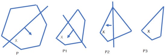
Figure 2.
ACCPM shrinking set.
At every iteration, the algorithm calculates the analytical center of the new working set defined and generated in the previous iteration. If this center of analysis is a a wailed solution, the algorithm is terminated, otherwise, the new plane is returned and added to the system. The algorithm finds a solution to the problem as the number of iterations increases, while the working set is shrinking.
4. System Model
A broadcast MIMO system with multiusers as shown in Figure 3 is considered in this work, where an N-antenna transmitter broadcasts confidential signals to K receivers each equipped with antennas through channel that are assumed to be random and follow a channel model of quasi-static flat-fading-type to ensure they are constant through the duration of interest. These signals are superimposed at the transmitter with beamforming vectors thus, the transmitted signal is so that the received signal at each receiver is:
where denotes the complex Gaussian noise at the kth receiver. Without the loss of generality, an assumption that considers the transmitted signal to be random with unit variance, and zero means that lead to , applying QPSK modulation. Accordingly, the received power at the kth receiver becomes:
where the second term represents the interference power at the kth receiver.
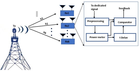
Figure 3.
Multi-user MIMO system.
First, the case of a single receiver (K = 1) is assumed which results in omitting the second term and reduces (3) to:
The value of is measured at the receiver at each time interval and compared with the previous value. Then, the receiver sends an or according to the comparison result that is represented by a one-bit feedback or at the transmitter according to the following comparison result
With the values, the transmitter estimates the covariance matrix of the channel using ACCPM. Accordingly, the analytic center that contains the query point can be determined using the following convex optimization problem
Note that P-1 is a convex optimization problem and can be solved using the interior point method or other convex optimization tools such as CVX [38]. Additionally, the constraint in (7) is to ensure that the resultant covariance channel matrix is positive semi-definite which is the inherent characteristic of the matrix.
The initial beamforming vector is generated randomly from the complex Gaussian distribution with zero mean and unit variance. The beamforming vector must be updated after each iteration using the following equation:
To satisfy the above equation, it is clear that must belong to the null space of . That is, let denote a vector of the null space of , then the beamforming vector is updated:
The above method is summarized in the following algorithm. This algorithm was implemented using MATLAB 2021 with a Razer Blade laptop (Razer, Inc., Irvine, CA, USA) with 8 GB RAM and a Core i7 processor (Intel Corporation, Santa Clara, CA, USA). It can implemented by any PC that can run MATLAB 2014, such as a PC with 4 GB RAM and a Core 2 Duo processor.
According to Algorithm 1, the simulation is terminated when the difference between the estimated covariance channel matrix and the actual covariance channel matrix is small enough or the number of time intervals exceeds the predefined value.
| Algorithm 1 CSI estimation for single user single beamforming vector |
Initialization: Set the maximum allowed error between the estimated and actual CSI () . . . . Evaluate using (7). Update beamforming vector using (9). Repeat
Until or |
To speed up the covariance channel matrix estimation, the receiver also compares the estimated power with the actual power at the same time interval and sends back an additional and signal to the transmitter. This signal is interpreted by the transmitter as a one-bit binary value according to the following inequality:
Combining (7) and (10), the new estimation convex optimization problem is formulated as:
where the beamforming vector of the above problem still must be updated according to (9).
Algorithm 1 can be slightly adjusted to estimate from P-2.
5. Multiple Beamforming Vectors
5.1. Orthogonal Vectors
Note that Equation (11) generates two cutting plans shown in Figure 4a to reduce the CSI estimation time, but there is no control on the generated cutting plane. Figure 4a shows no effect because the generated cutting plane is approximately the same, while in Figure 4b,c the two generated cutting planes are approximately perpendicular. To control the generated cutting planes, more than one beamforming vector can be sent by the transmitter.
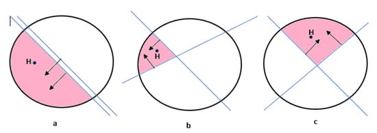
Figure 4.
Multiplecutting planes through orthogonal beamforming.
These beamforming vectors should be orthogonal to generate orthogonal cutting planes so that they can be easily separated by the receiver. Vectors are orthogonal if the dot product between any two vectors is equal to zero. The Gram-Schmidt process [39,40] can be used to orthogonalize the beamforming vectors, which is a common process in linear algebra to generate an orthogonal vector set (where Z represents the number of the orthogonal vector needed) from a non-orthogonal vector set . The Gram-Schmidt process is given as follows:
where represents the inner product of two vectors.
On the receiver side, a comparison is performed to extract is the corresponding vector, which is sent to the transmitter as feedback bits.
The transmitter utilizes these values to estimate the channel covariance matrix. Accordingly, the following convex optimization problem is formulated:
The beamforming vectors are updated using the null space of the estimated covariance channel matrix. Since each vector uses different null spaces, the number of vectors used to estimate the matrix is equal to the number of null spaces, which is determined and restricted by the number of antennas at the transmitter and receiver sides.
The following algorithm summarizes the procedure to estimate using multiple orthogonal beamforming vectors (Algorithm 2).
| Algorithm 2 CSI estimation using orthogonal beamforming vector |
Initialization: Set the maximum allowed error between estimated and actual CSI () . ). (12). . Evaluate using (14). Update beamforming vector using (9). Repeat
Until or |
5.2. Non-Orthogonal Vectors
In this scenario, a single user can be considered as multiple receivers, where each antenna is considered as an independent receiver, and a signal from the transmitter is sent to each antenna. As a result, each column of the channel covariance matrix , becomes the channel vector of each receiver. In this case, the transmitter sends M signals and a comparison is performed at each receiving antenna. The comparison results are fed back to the transmitter.
According to the results from (15), the transmitter uses the following optimization to estimate .
In this case, the beamforming vector is updated by adding the principal eigenvector of which is obtained by using decomposition of to the corresponding vector.
The simulation of P-4 can be performed with the assistance of Algorithm 3.
| Algorithm 3 CSI estimation using multiple non-orthogonal vectors |
Initialization: Set the maximum allowed error between the estimated and actual CSI () . . . . (16). Update beamforming vectors by adding the previous vector to the corresponding principle in vector. Repeat
Until or |
6. Multiple Users
When there are multiple users (i.e., ), the transmitter can either send multiple beamforming vectors to multiple users or send only one beamforming vector by considering all users as a single user.
6.1. Multiple Users Multiple Beamforming Vectors
In this case, the received power at each user is determined by (3). At each time instance, the power comparison is performed as:
The receivers feed back the values of s to the transmitter for ACCPM-based CSI estimation, which is performed by solving the following convex optimization problem:
All users’ CSI is determined separately by solving K convex optimization problems in (18).
Then, the K beamforming vectors are updated by determining the K null space of CSI using:
Algorithm 1 with multiple optimization problems is applied to the above problem.
6.2. Multiple Users Single Beamforming Vector
In this scenario, the transmitter sends a single beamforming vector to all users by finding the common null space of these receivers [41,42]. Let denote the total number of antennas across all receivers, the bmatrix must be found, which represents the common channel between the transmitter and all receivers. Specifically, the received signal can be written as:
where is the total noise between the transmitter and all receivers. Let , then (20) becomes . Then, the comparison performed at the fusion centre is:
Then, according to the values of , the transmitter determines the channel covariance matrix using the following optimization:
Finally, the beamforming vector is updated using the null space of . It is worth noting that, since the rank of the covariance channel matrix is min , the covariance channel matrix has null space only if .
The null space of is found by finding the singular value decomposition (SVD) of , i.e.,
where represents the first M right singular vectors and denotes the orthogonal basis null space of .
The method can be implemented following the procedure in Algorithm 4.
| Algorithm 4 CSI estimation for multi-user single beamforming vector |
Initialization: Set the maximum allowed error between the estimated and actual CSI () . . . (22). . Repeat
Until or |
7. Numerical Results
This section provides the simulation results to illustrate the performance of the proposed ACCPM methods. The initial beamforming vectors for all cases are generated randomly from the complex Gaussian distribution with zero mean and unit covariance. Each simulation result is averaged over 500 trials.
The actual correlation matrix is determined by and the error in the estimated covariance matrix is , where is the estimated covariance matrix. The beamforming vector is extracted by eigen-decomposition of the estimated covariance matrix where the principle Eigenvector is the optimal beamforming vector.
When , Figure 5 shows the convergence (i.e., channel estimation error versus estimation time) of our proposed solution under different MIMO configurations. We can see that, with fixed number of receiving antennas, the channel estimation time increases with the number of transmitter antennas. This is expected because the complexity of estimating the channel covariance matrix increases with the number of antennas. Eventually, our channel estimation solution converges in all cases.
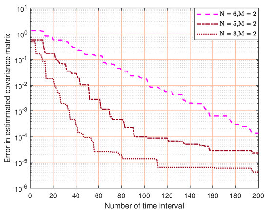
Figure 5.
The convergence of channel covariance matrix estimation for a different number of transmitting antennas.
When , Figure 6 demonstrates the transmitted signal power versus the learning time. In all cases the power drops to zero at the end of the learning period. This is because we use the null space vector of the estimated channel covariance matrix, which converges to the actual channel covariance matrix. Similar to Figure 3, we also find that the convergence time increases with the number of transmitter antennas.
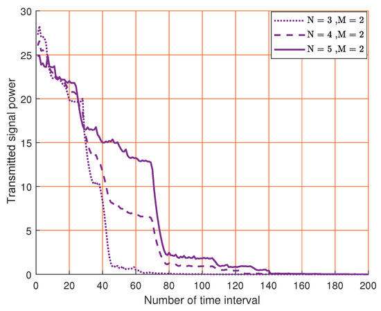
Figure 6.
The convergence of the transmitted signal power for different number of transmitting antennas.
When , Figure 7 shows the normalized error in estimating the channel covariance matrix versus the estimation time for a different number of transmitting antennas. We see that the convergence time is reduced as the number of receiving antennas is increased, because the number of estimating sensors to estimate the parameters increased.
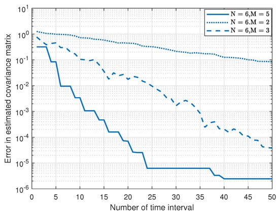
Figure 7.
Normalized channel estimation error versus estimation time for different number of receiving antennas.
Figure 8 explains the proposed two cutting planes as compared with the results in [31]. We can see that our proposed method outperforms that in [31]. This is because as the number of cutting planes increase, the time interval to estimate the channel decreases, as explained in Figure 5.
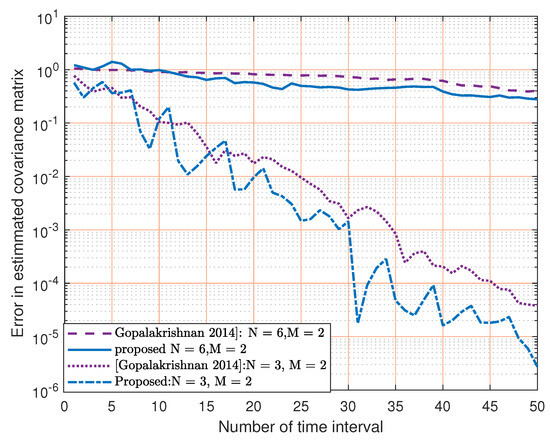
Figure 8.
Normalized error of estimated covariance matrix for the two proposed cutting planes versus [31] for different MIMO configurations.
When and , Figure 9 compares the performance of our proposed method with [32]. We can see that the performance of our method improves significantly as the number of orthogonal vectors increases, dividing the convex set into halves, quarters and eventually approaching the estimated channel matrix. In particular, our method outperforms the 10-bit method in [32] with three proposed vectors.
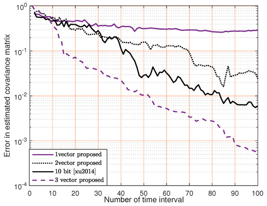
Figure 9.
Performance comparison of our orthogonal cutting plane method versus the multiple-bit method in [32].
Figure 10 shows the transmitting power versus the channel estimation time for non-orthogonal vectors. We observe that as the number of vectors increases, the power quickly comes to a steady state.
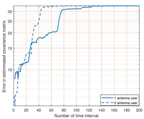
Figure 10.
Transmitting power for non-orthogonal vector.
Figure 11 shows the convergence of our method in a multi-user scenario, and it shows that our method sometimes outperforms the method in [30].

Figure 11.
Error in estimated covariance matrix versus time interval for the multiuser case [30].
For the purpose of verification of the method, the method is tested using one of the standard channel models: the scattering channel [43] that is used to test the method with a single user using P-1 with different settings in Table 2, where d represents the spacing between antenna elements in terms of wavelength , and D is the distance between the transmitter and receiver. The optimization problem (P-1) is solved under different channel settings and the results are shown in Figure 12, which shows the convergence of our method. We can also see that the channel estimation time increases with the number of transmitting antennas because more parameters need to be estimated.
Table 2.
Scattering channel with different settings.
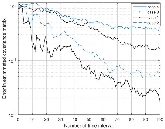
Figure 12.
Channel covariance matrix estimation with different scattering channels.
Finally, for a multiple user case with a standard channel, the winner channel model is tested [44] using P-6 where a single base station is assumed to communicate with two mobile stations and for a different type of MIMO system, as illustrated in Table 3.
Table 3.
Winner channel model with different settings.
Where N represents the number of transmitting antenna in the base station, represents the number of antenna in mobile station 1 and, is the number of antenna in mobile station 2. For more details on the configuration of the winner channel, please refer to [45].
Figure 13 indicates the convergence of our method in P-6 when the winner channel model is used. Additionally, the results satisfy the previous results where we see that as the number of transmitting antenna increase, the time interval required to achieve convergence increases too. This is due to the fact that the channel matrix dimension increases which leads to an increasing number of the elements needed to be estimated. At the other side, as the number of receiving antenna increases, the time interval required to achieve convergence decreases. This is because the sensing element at the receiver side increases, which is responsible for the estimation even when the dimensions of the matrix needed to be estimated are larger.
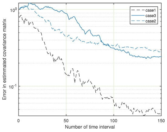
Figure 13.
Channel covariance matrix estimation with different winner channel models.
8. Conclusions
The paper demonstrates different methods of using ACCPM for channel covariance matrix estimation in various MIMO systems including single user, multiuser, and multi beamforming vectors. The simulation results show that the proposed methods not only converge but also outperform existing benchmark methods. In particular, the use of null space during the learning phase is a better choice to reduce the power consumption. Using ACCPM, the learning is achieved at the transmitter side and requires little feedback from the receiver. Additionally, the transmitter starts learning without any information about the estimated CSI. The effectiveness of the method was corroborated by applying it to standard channel models. The method can be considered in terms of artificial intelligent as a simple classification problem or can be solved using prediction methods. This can be considered for future studies, where it can be improved further by reducing the feedback time intervals. Additionally, it could be tested for all channel models and the probabilistic mathematical concepts could be considered for future work.
Author Contributions
Conceptualization, A.A.-A.; Methodology, A.A.-A.; Software, A.A.-A., I.R.K.A.-S. and L.A.; Validation, A.A.-A. and I.R.K.A.-S.; Formal analysis, A.A.-A., S.K.A. and H.L.; Resources, I.R.K.A.-S. and L.A.; Writing—original draft, A.A.-A. and S.K.A.; Writing—review & editing, I.R.K.A.-S., H.L. and L.A.; Visualization, L.A.; Supervision, H.L. All authors have read and agreed to the published version of the manuscript.
Funding
This work was partially funded by the Ministry of Higher Education in Iraq through the research grant project in cooperation with the University of Louisville, USA.
Informed Consent Statement
Not applicable.
Data Availability Statement
Not applicable.
Conflicts of Interest
The authors declare no conflict of interest.
References
- Love, D.J.; Heath, R.W.; Santipach, W.; Honig, M.L. What is the value of limited feedback for MIMO channels? IEEE Commun. Mag. 2004, 42, 54–59. [Google Scholar] [CrossRef]
- Song, H.; Wen, H.; Liao, R.-F.; Chen, Y.; Chen, S. Outage constrained secrecy rate maximization for MIMOME multicast wiretap channels. IEEE Wirel. Commun. Lett. 2018, 8, 657–660. [Google Scholar] [CrossRef]
- Yuan, Y.; Ding, Z. Outage constrained secrecy rate maximization design with SWIPT in MIMO-CR systems. IEEE Trans. Veh. Technol. 2017, 67, 5475–5480. [Google Scholar] [CrossRef]
- Al-Asadi, A.; Al-Amidie, M.; Micheas, A.C.; McGarvey, R.G.; Islam, N.E. Worst case fair beamforming for multiple multicast groups in multicell networks. IET Commun. 2019, 13, 664–671. [Google Scholar] [CrossRef]
- Al-Amidie, M.; Al-Asadi, A.; Humaidi, A.J.; Al-Dujaili, A.; Alzubaidi, L.; Farhan, L.; Fadhel, M.A.; McGarvey, R.G.; Islam, N.E. Robust Spectrum Sensing Detector Based on MIMO Cognitive Radios with Non-Perfect Channel Gain. Electronics 2021, 10, 529. [Google Scholar] [CrossRef]
- Al-Asadi, A.; Al-Amidie, M.; Alwane, S.K.; Albehadili, H.M.; McGarvey, R.G.; Islam, A.N.E. Robust underlay cognitive network download beamforming in multiple users, multiple groups multicell scenario. IET Commun. 2021, 14, 3934–3943. [Google Scholar] [CrossRef]
- Shehzad, M.; Rose, L.; Assaad, M. A Novel Algorithm to Report CSI in MIMO-Based Wireless Networks. In Proceedings of the ICC International Conference of Communication, Online, 14–23 June 2021. [Google Scholar]
- Mahmood, A.; Ashraf, M.I.; Gidlund, M.; Torsner, J. Over-the-Air Time Synchronization for URLLC: Requirements, Challenges and Possible Enablers. In Proceedings of the 2018 15th International Symposium on Wireless Communication Systems (ISWCS), Lisbon, Portugal, 28–31 August 2018; pp. 1–6. [Google Scholar]
- Lakshminarayana, S.; Assaad, M.; Debbah, M. Coordinated multicell beamforming for massive MIMO: A random matrix approach. IEEE Trans. Inf. Theory 2015, 61, 3387–3412. [Google Scholar] [CrossRef]
- Zhou, X.; Song, L.; Zhang, Y. Physical Layer Security in Wireless Communications; CRC Press: Boca Raton, FL, USA, 2013. [Google Scholar]
- Cheema, M.A.; Shehzad, M.K.; Qureshi, H.K.; Hassan, S.A.; Jung, H. A drone-aided blockchain-based smart vehicular network. IEEE Trans. Intell. Transp. Syst. 2021, 22, 4160–4170. [Google Scholar] [CrossRef]
- Baeza, V.M.; Armada, A.G. Orthogonal versus Non-Orthogonal multiplexing in Non-Coherent Massive MIMO Systems based on DPSK. In Proceedings of the 2021 Joint European Conference on Networks and Communications & 6G Summit (EuCNC/6G Summit), Porto, Portugal, 8–11 June 2021; pp. 101–105. [Google Scholar]
- Nguyen, L.V.; Swindlehurst, A.L.; Nguyen, D.H.N. SVM-based channel estimation and data detection for one-bit massive MIMO systems. IEEE Trans. Signal Process. 2021, 69, 2086–2099. [Google Scholar] [CrossRef]
- Gajjar, V.; Kosbar, K. CSI Estimation Using Artificial Neural Network; International Foundation for Telemetering: San Diego, CA, USA, 2019. [Google Scholar]
- Kang, X.-F.; Liu, Z.-H.; Yao, M. Deep learning for joint pilot design and channel estimation in MIMO-OFDM systems. Sensors 2022, 22, 4188. [Google Scholar] [CrossRef]
- Del Rosario, M.; Ding, Z. Learning-Based MIMO Channel Estimation under Practical Pilot Sparsity and Feedback Compression. IEEE Trans. Wirel. Commun. 2022, 22, 1161–1174. [Google Scholar] [CrossRef]
- Wen, C.; Shih, W.; Jin, S. Deep learning for massive MIMO CSI feedback. IEEE Wirel. Commun. Lett. 2018, 7, 748–751. [Google Scholar] [CrossRef]
- Li, Y.; Yin, Q.; Sun, L.; Chen, H.; Wang, H.-M. A channel quality metric in opportunistic selection with outdated CSI over Nakagami-m fading channels. IEEE Trans. Veh. Technol. 2012, 61, 1427–1432. [Google Scholar] [CrossRef]
- Cheng, L.; Shi, Q. Towards Overfitting Avoidance: Tuning-free Tensor-aided Multi-user Channel Estimation for 3D Massive MIMO Communications. IEEE J. Sel. Top. Signal Process. 2021, 15, 832–846. [Google Scholar] [CrossRef]
- Gao, Z.; Dai, L.; Wang, Z.; Chen, S. Spatially common sparsity-based adaptive channel estimation and feedback for FDD massive MIMO. IEEE Trans. Signal Process. 2015, 63, 6169–6183. [Google Scholar] [CrossRef]
- Fan, D.; Gao, F.; Wang, G.; Zhong, Z.; Nallanathan, A. Angle domain signal processing-aided channel estimation for indoor 60-GHz TDD/FDD massive MIMO systems. IEEE J. Sel. Areas Commun. 2017, 35, 1948–1961. [Google Scholar] [CrossRef]
- Xu, W.; Cui, Y.; Zhang, H.; Li, G.Y.; You, X. Robust beamforming with partial channel state information for energy efficient networks. IEEE J. Sel. Areas Commun. 2015, 33, 2920–2935. [Google Scholar] [CrossRef]
- Noam, Y.; Manolakos, A.; Goldsmith, A.J. Null space learning with interference feedback for spatial division multiple access. IEEE Trans. Wirel. Commun. 2014, 13, 5699–5715. [Google Scholar] [CrossRef]
- Loyka, S.; Charalambous, D. Novel matrix singular value inequalities and their applications to uncertain MIMO channels. IEEE Trans. Inf. Theory 2015, 61, 6623–6634. [Google Scholar] [CrossRef]
- Gao, F.; Zhang, R. Design of learning-based MIMO cognitive radio systems. IEEE Trans. Veh. Technol. 2010, 59, 1707–1720. [Google Scholar]
- Yi, H. Nullspace-based secondary joint transceiver scheme for cognitive radio MIMO networks using second-order statistics. In Proceedings of the 2010 IEEE International Conference on Communications, Cape Town, South Africa, 23–27 May 2010; pp. 1–5. [Google Scholar]
- Patel, A.; Biswas, S.; Jagannatham, A.K. Optimal GLRT-based robust spectrum sensing for MIMO cognitive radio networks with CSI uncertainty. IEEE Trans. Signal Process. 2015, 64, 1621–1633. [Google Scholar] [CrossRef]
- Liu, B.; Cheng, Y.; Zhou, Q. Robust rank-two beamforming for multicell multigroup multicast. IET Commun. 2016, 10, 283–291. [Google Scholar] [CrossRef]
- Gong, J. Base Station Cooperations Under Imperfect Conditions. In Encyclopedia of Wireless Networks; Springer: Cham, Switzerland, 2020. [Google Scholar]
- Xu, J.; Zhang, R. Energy beamforming with one-bit feedback. IEEE Trans. Signal Process. 2014, 62, 5370–5381. [Google Scholar] [CrossRef]
- Gopalakrishnan, B.; Sidiropoulos, N.D. Cognitive transmit beamforming from binary CSIT. IEEE Trans. Wirel. Commun. 2014, 14, 895–906. [Google Scholar] [CrossRef]
- Xu, J.; Liu, L.; Zhang, R. Multiuser MISO beamforming for simultaneous wireless information and power transfer. IEEE Trans. Signal Process. 2014, 62, 4798–4810. [Google Scholar] [CrossRef]
- Ghosh, A.; Kim, M. THz channel sounding and modeling techniques: An overview. IEEE Access 2023, 11, 17823–17856. [Google Scholar] [CrossRef]
- Almers, P.; Bonek, E.; Burr, A.; Czink, N.; Debbah, M.; Degli-Esposti, V.; Hofstetter, H.; Kyösti, P.; Laurenson, D.; Matz, G.; et al. Survey of channel and radio propagation models for wireless MIMO systems. EURASIP J. Wirel. Commun. Netw. 2007, 2007, 019070. [Google Scholar] [CrossRef]
- Imoize, A.L.; Ibhaze, A.E.; Atayero, A.A.; Kavitha, K.V.N. Standard propagation channel models for MIMO communication systems. Wirel. Commun. Mob. Comput. 2021, 2021, 8838792. [Google Scholar] [CrossRef]
- Feng, R.; Wang, C.-X.; Huang, J.; Gao, X.; Salous, S.; Haas, H. Classification and comparison of massive MIMO propagation channel models. IEEE Internet Things J. 2022, 19, 23452–23471. [Google Scholar] [CrossRef]
- Sun, J.; Toh, K.-C.; Zhao, G. An analytic center cutting plane method for semidefinite feasibility problems. Math. Oper. Res. 2002, 77, 332–346. [Google Scholar] [CrossRef][Green Version]
- Boyd, S.; Vandenberghe, L. Convex Optimization; Cambridge University Press: Cambridge, UK, 2004. [Google Scholar]
- Alkhateeb, A.; Heath, R.W. Frequency selective hybrid precoding for limited feedback millimeter wave systems. IEEE Trans. Commun. 2016, 64, 1801–1818. [Google Scholar] [CrossRef]
- Li, X.; Alkhateeb, A. Deep learning for direct hybrid precoding in millimeter wave massive MIMO systems. In Proceedings of the 2019 53rd Asilomar Conference on Signals, Systems, and Computers, Pacific Grove, CA, USA, 3–6 November 2019; pp. 800–805. [Google Scholar]
- Spencer, Q.H.; Swindlehurst, A.L.; Haardt, M. Zero-forcing methods for downlink spatial multiplexing in multiuser MIMO channels. IEEE Trans. Signal Process. 2004, 52, 461–471. [Google Scholar] [CrossRef]
- Zhan, J.; Dong, X. Interference Cancellation Aided Hybrid Beamforming for mmWave Multi-User Massive MIMO Systems. IEEE Trans. Veh. Technol. 2021, 70, 2322–2336. [Google Scholar] [CrossRef]
- Available online: https://www.mathworks.com/help/phased/ref/scatteringchanmtx.html (accessed on 4 June 2023).
- Available online: https://www.mathworks.com/help/comm/ref/winner2.layoutparset.html (accessed on 7 June 2023).
- Kyösti, P.; Meinilä, J.; Hentilä, L.; Zhao, X.; Jämsä, T.; Schneider, C.; Narandzić, M.; Milojević, M.; Hong, A.; Ylitalo, J.; et al. IST-4-027756 WINNER II D1. 1.2 V1. 2 WINNER II Channel Models. EBITG, TUI, UOULU, CU/CRC, NOKIA. Technical Report. 2007. Available online: http://signserv.signal.uu.se/Publications/WINNER/WIN2D112.pdf (accessed on 9 June 2023).


Disclaimer/Publisher’s Note: The statements, opinions and data contained in all publications are solely those of the individual author(s) and contributor(s) and not of MDPI and/or the editor(s). MDPI and/or the editor(s) disclaim responsibility for any injury to people or property resulting from any ideas, methods, instructions or products referred to in the content. |
© 2023 by the authors. Licensee MDPI, Basel, Switzerland. This article is an open access article distributed under the terms and conditions of the Creative Commons Attribution (CC BY) license (https://creativecommons.org/licenses/by/4.0/).