
Pulsed-Mode Magnetic Field Measurements with a Single Stretched Wire System

 , , , and
Abstract
1. Introduction
2. Measurement Principle
2.1. Static SSW
2.2. Pulsed SSW
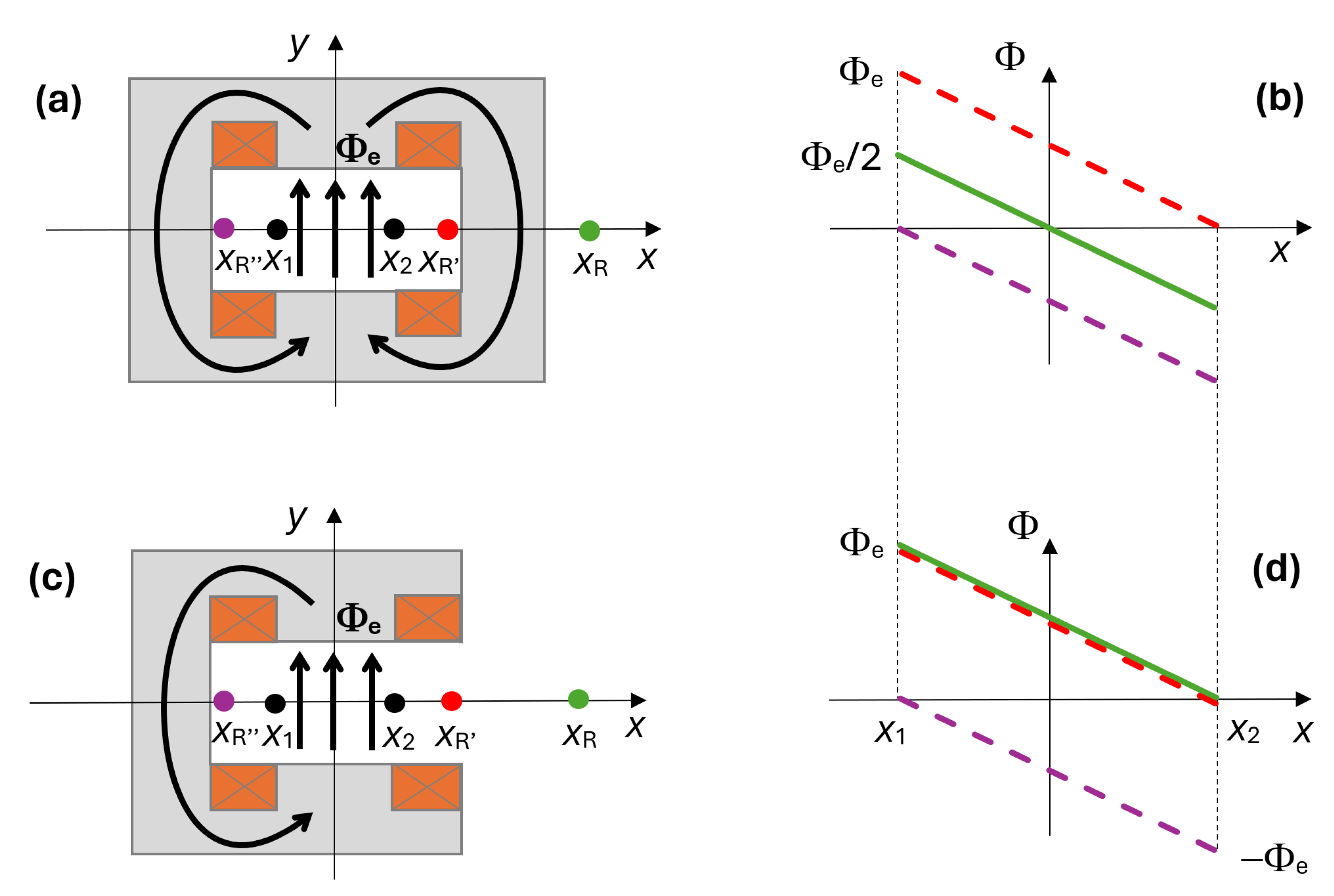
- Window-frame dipole (inset a, b): When the return wire is external to the magnet (), the measured flux changes antisymmetrically with respect to the origin, reaching, at both ends, the same absolute value . If, instead, the return wire is inside the magnet gap at either position or due to the symmetry of the yoke, the linked flux will be ∼0 at one end and reach the maximum value ∼ at the other.
- C-shaped dipole (inset c, d): If the return wire is placed on the side where the yoke is open, either externally ( ) or internally ( ) to the gap, the measured flux will behave identically i.e., it will swing from the maximum value ∼ to ∼0; if, instead, the return is moved on the closed side of the yoke (), the sign of flux will be opposite as the curve is shifted by .
2.3. Combined SSW
2.4. Induction Coil
- Flip-coil method: The coil is first positioned flat in its central rest position inside the magnet’s gap (roll angle ), then it is flipped upside down () while measuring the induced voltage . The final flux linkage will be equal and opposite to the initial one, and we can derive the following:where the integration bounds correspond to mechanically stable coil configurations. The result, in principle, does not depend upon the precise law of motion followed, even if some translation is unwittingly superposed to the rotation. The main practical difficulty is turning the coil quickly enough to avoid the build-up of integrator drift while at the same time ensuring that the initial and final configurations are not offset in any direction. Mainly for this reason, a suitable nonmagnetic, nonconducting, rotating, mechanical support should be preferred to manual operation.
- Fixed coil method: We keep the coil fixed and instead ramp the current starting from zero up to its desired value, to obtain the flux change:This method is the most rapid and practical since it does not involve any coil handling; however, the measurement is blind to the initial flux . This is typically associated with a remanent field in the iron poles, which depends upon the previous magnetization history and can be of the order of a few milliteslas. Ideally, a demagnetization cycle should be applied before the measurement, but doing so requires bipolar power converters, which are not always available. In the alternative, must be measured independently, for example, by the flip-coil method. Another independent measurement of could be obtained with the static SSW method by scaling the results with the appropriate number of induction coil turns. However, the measured flux will not be entirely consistent with Equation (16), since the wire is much more straight than the coil windings, at least horizontally. Fortunately, the resulting error is often negligible since the integrated remanent field is very small, typically at least two orders of magnitude below the lowest level of interest (corresponding to beam injection). The value thus obtained is then added to the pulsed measurement to derive the absolute flux:The same can be reused multiple times for fixed coil measurements at different current levels. Doing so, however, requires that a stable hysteresis cycle be followed to ensure repeatability, as we have performed in the present work.
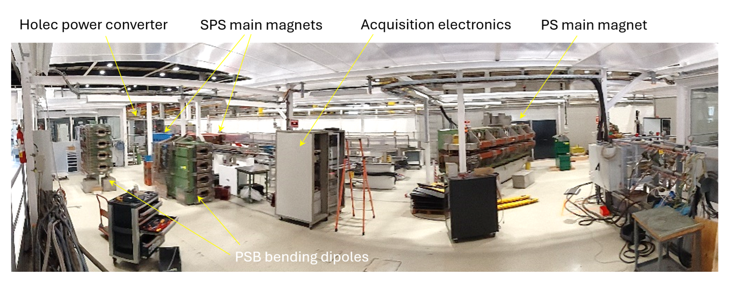
3. Test Setup
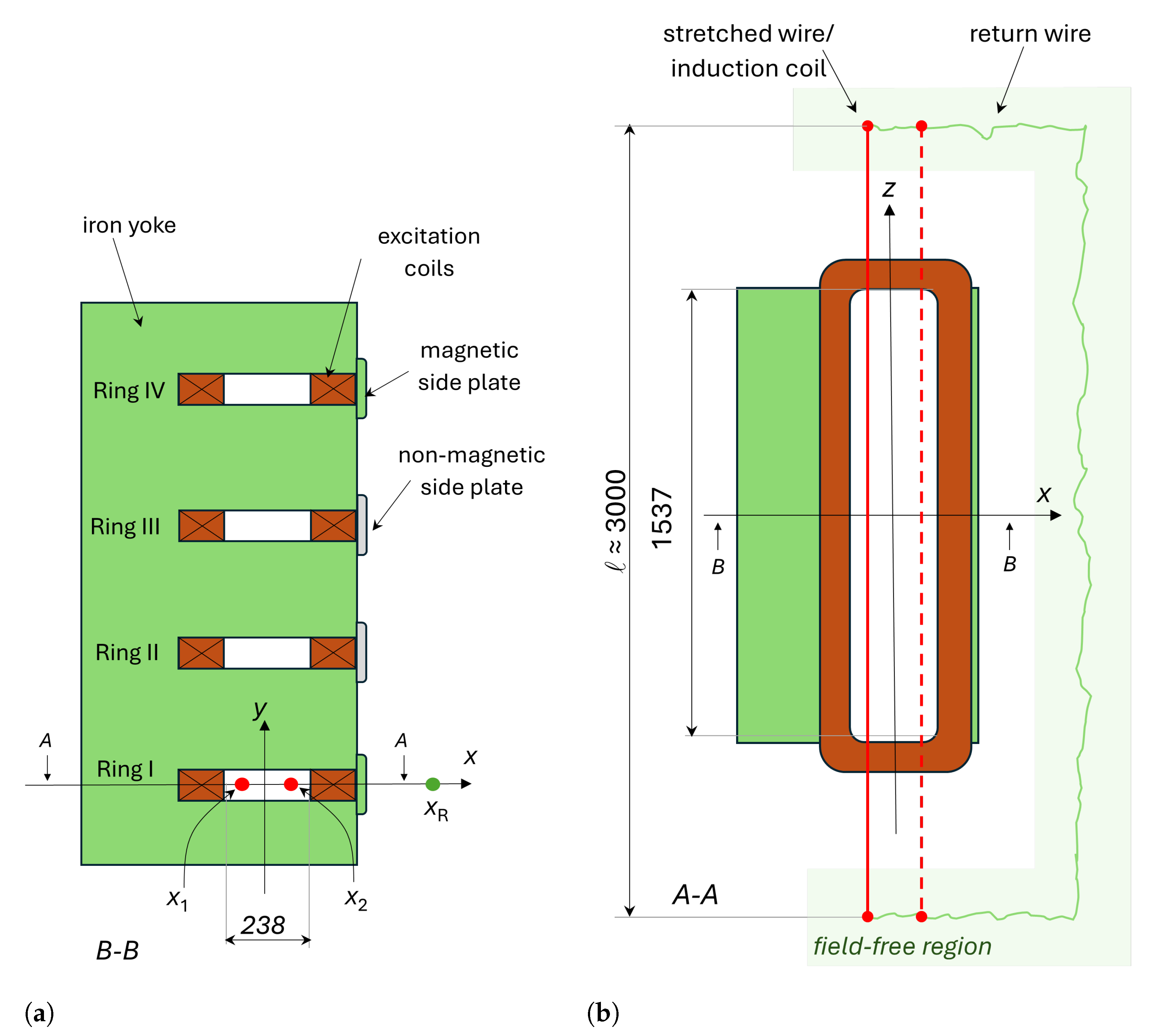
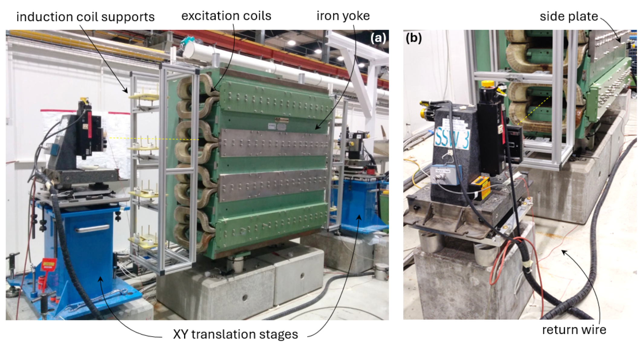
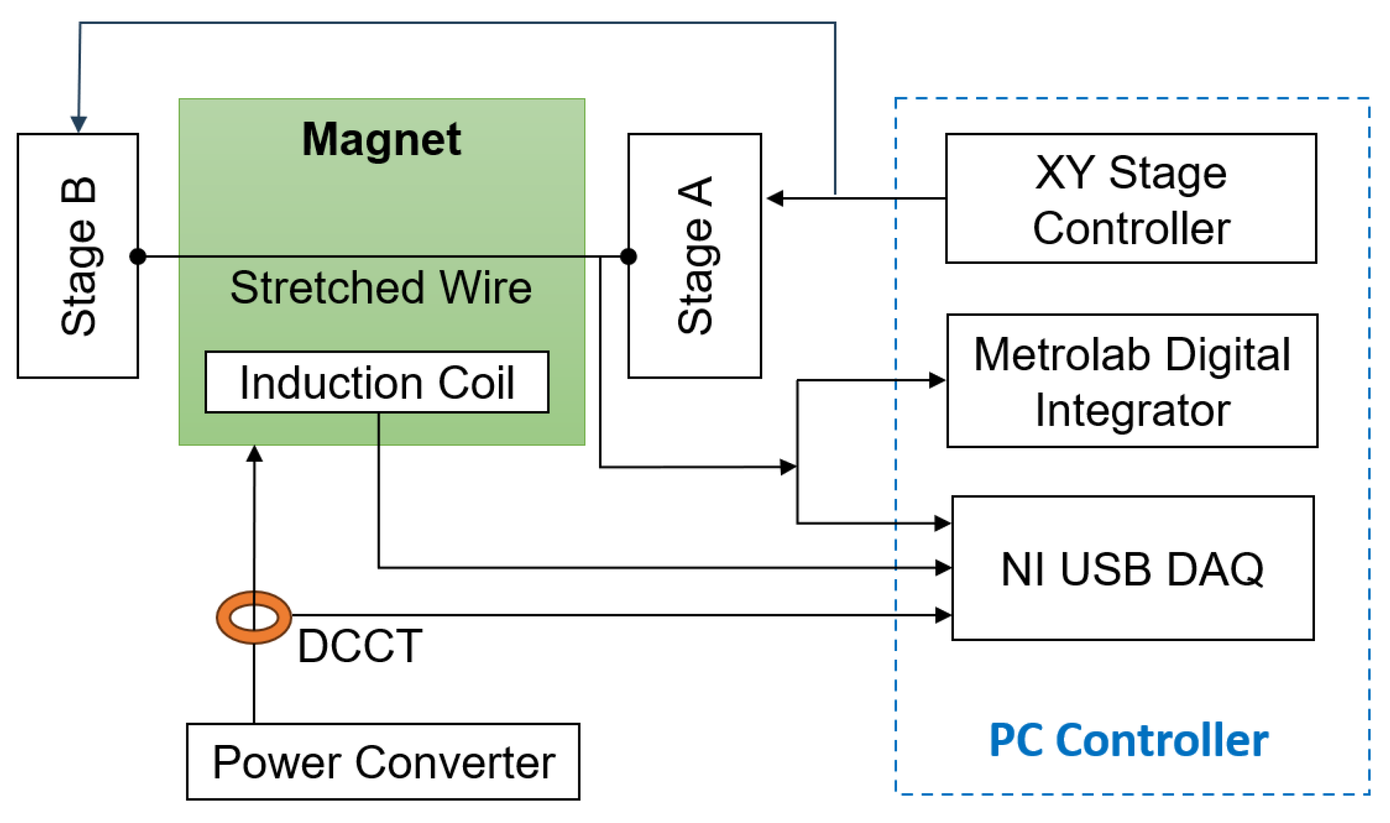
3.1. SSW Setup
3.2. Induction Coil
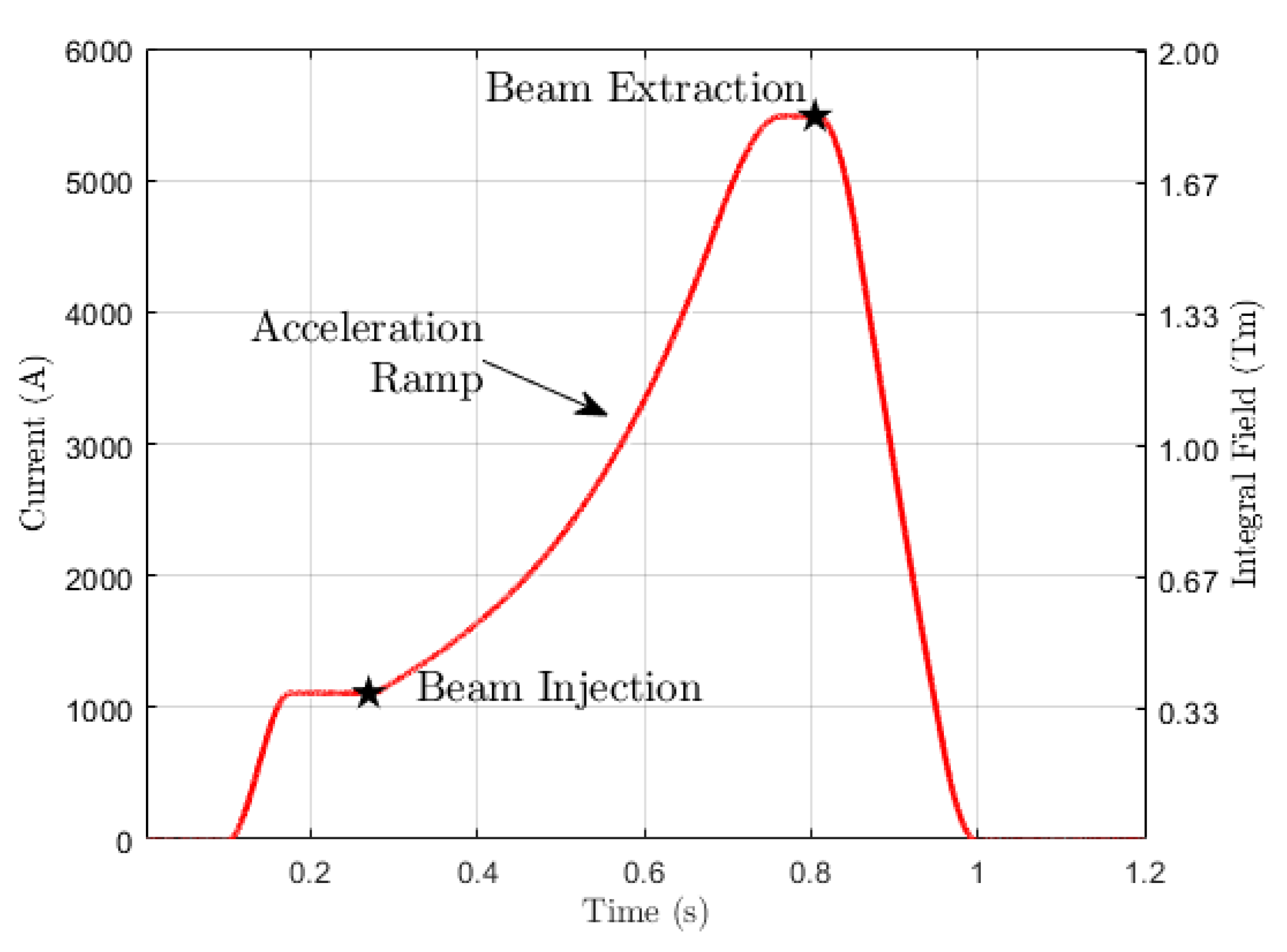
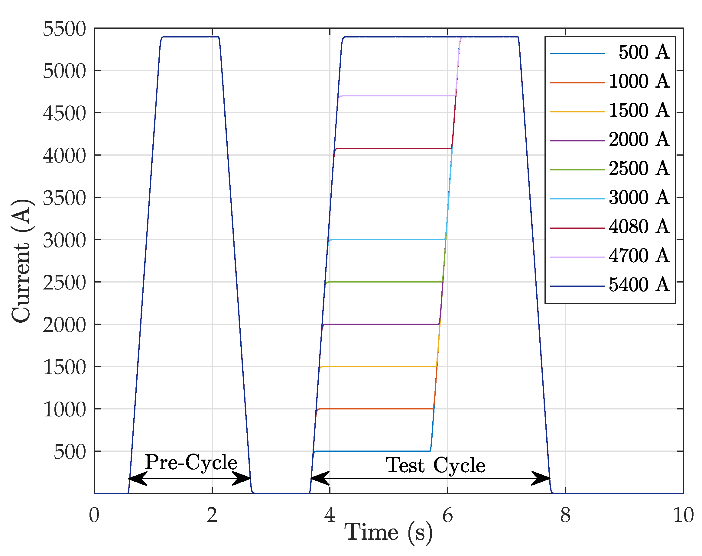
3.3. Magnet Powering
4. Measurement Results and Analysis
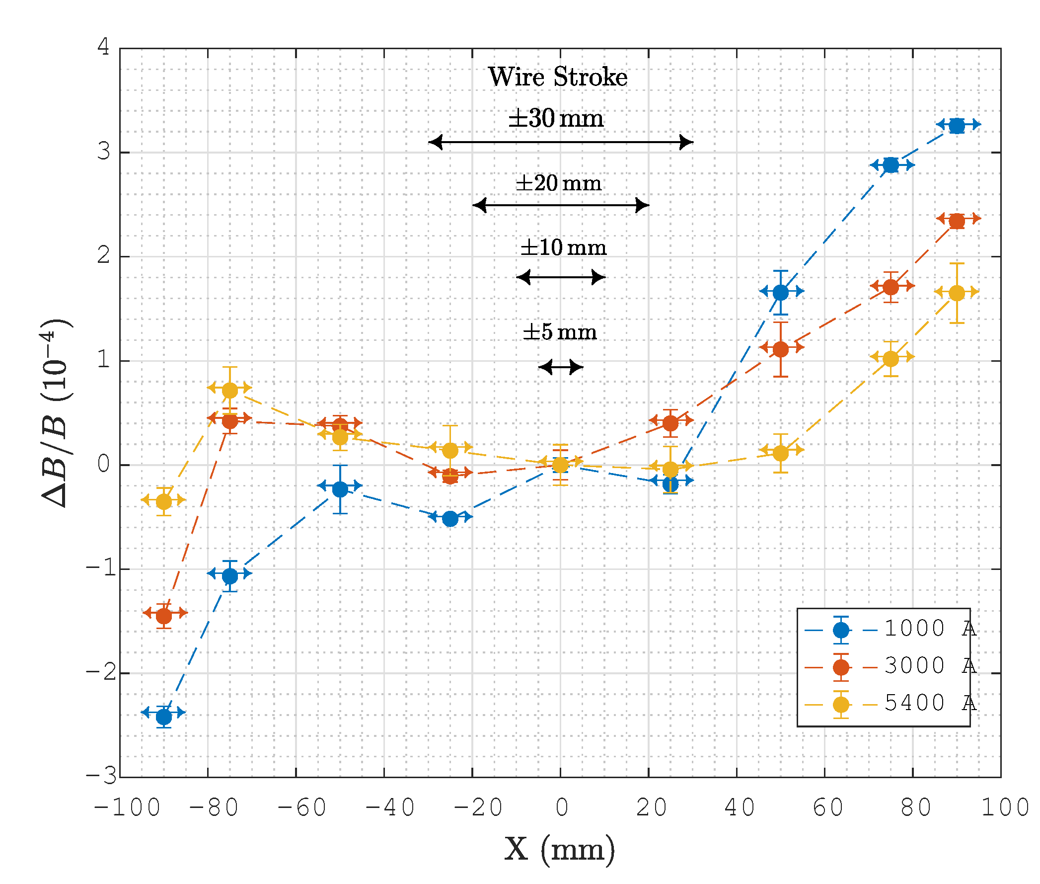
4.1. Field Uniformity
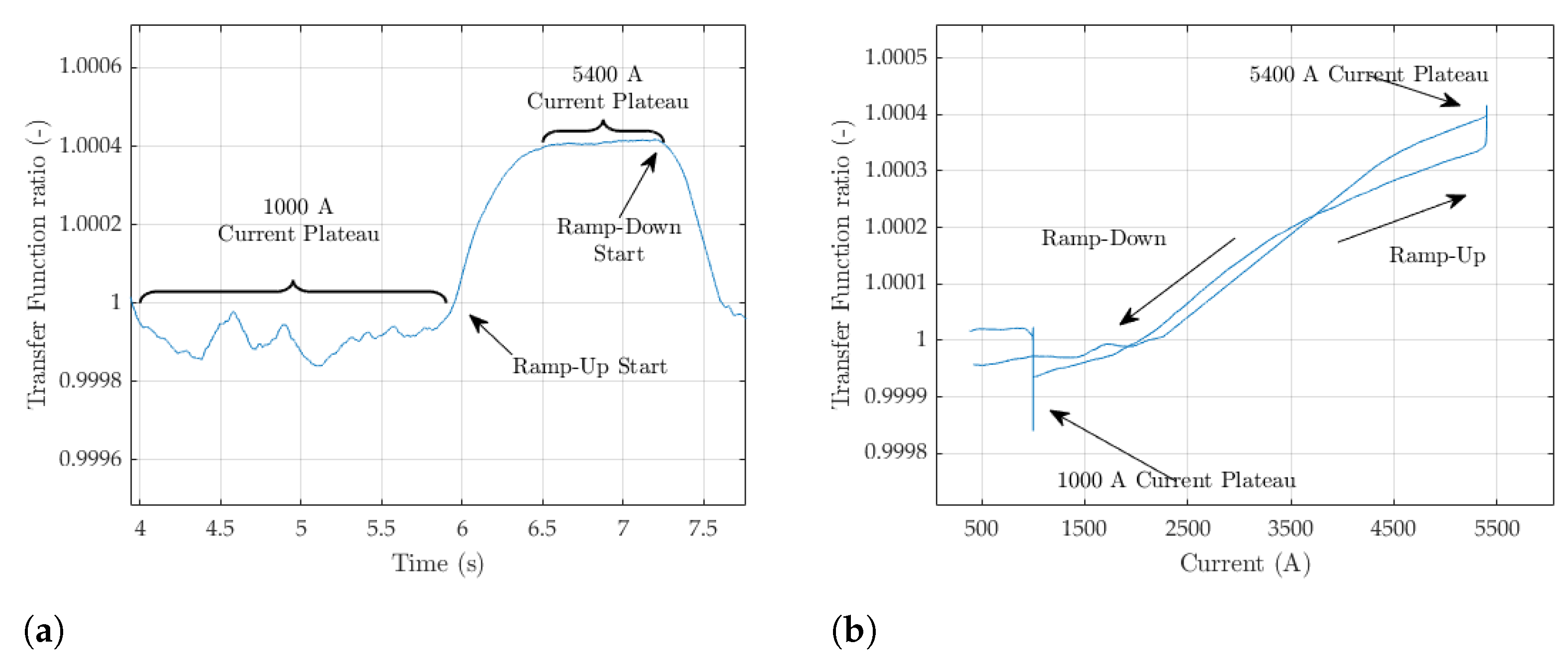
4.2. Pulsed SSW Results
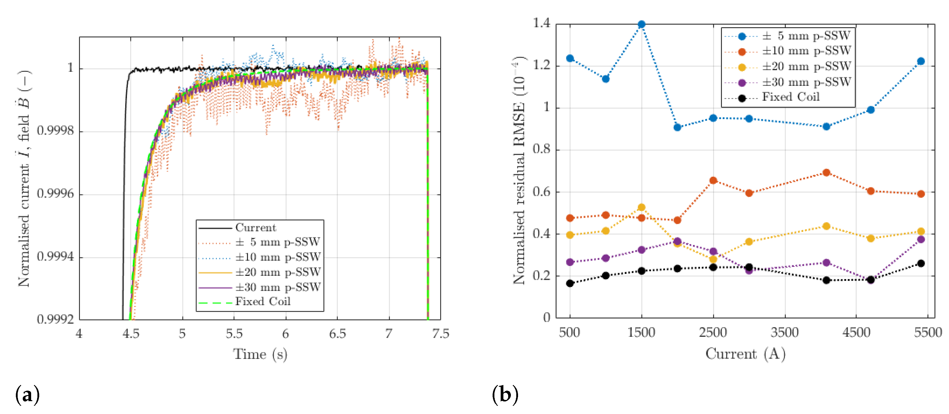
4.3. Noise Analysis
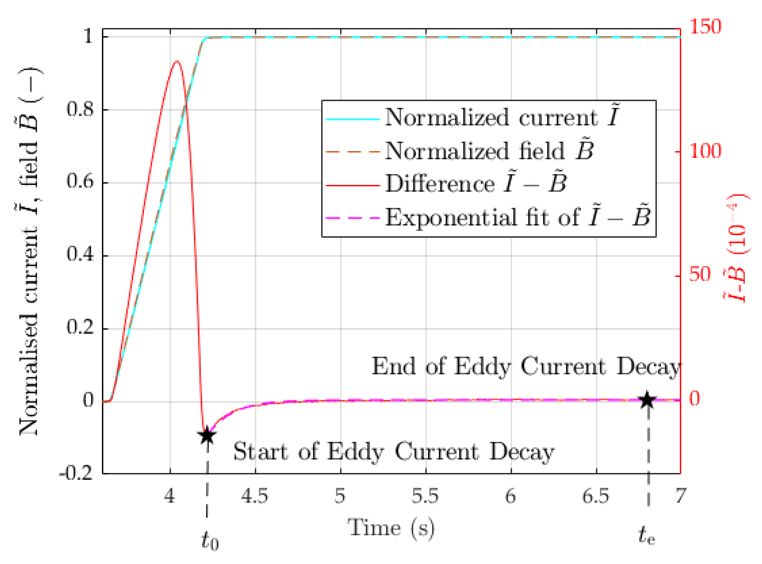
4.4. Eddy Current Decay Transient
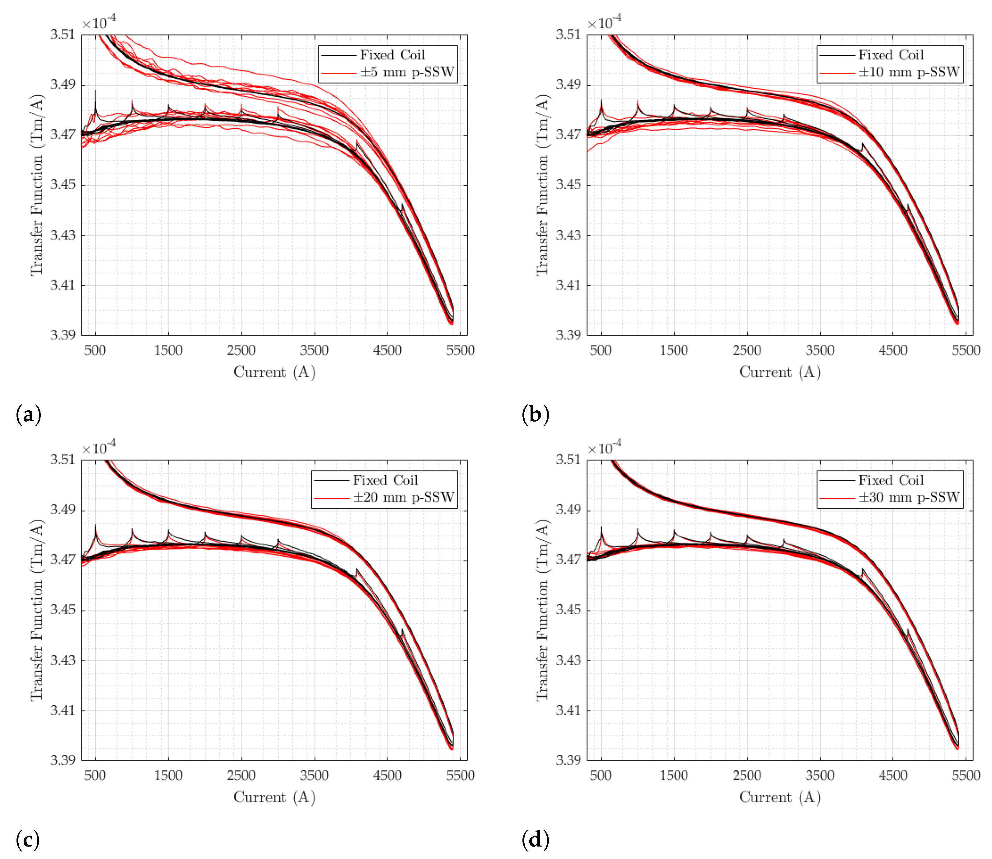
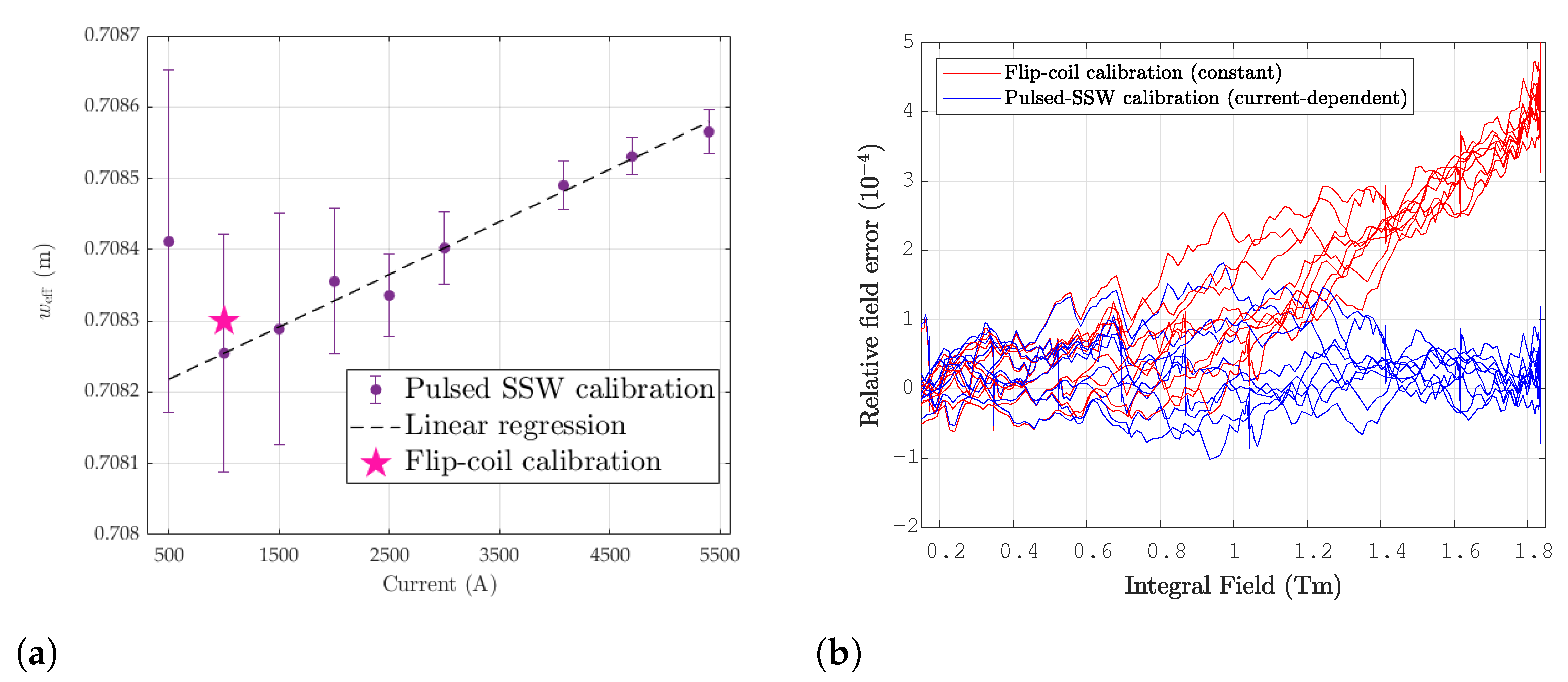
4.5. Comparison with Static SSW

| Current (A) | Integral Field (Tm) | Integral Transfer Function | Induction Coil Calibration (mm) | |||
|---|---|---|---|---|---|---|
| s-SSW | c-SSW | s-SSW | c-SSW | s-SSW | c-SSW | |
| 0 | - | - | - | - | - | |
| 500 | - | |||||
| 1000 | ||||||
| 1500 | - | |||||
| 2000 | - | |||||
| 2500 | - | |||||
| 3000 | - | |||||
| 4080 | - | - | - | |||
| 4700 | - | - | - | |||
| 5400 | - | - | - | |||
4.6. Comparison with the Fixed Coil Setup
5. Conclusions and Future Work
Author Contributions
Funding
Data Availability Statement
Acknowledgments
Conflicts of Interest
References
- Bryant, P.; Johnsen, K. The Principles of Circular Accelerators and Storage Rings; Cambridge University Press: Cambridge, UK, 2005. [Google Scholar] [CrossRef]
- Zickler, T. Basic design and engineering of normal-conducting, iron-dominated electromagnets. In Proceedings of the 2009 CAS-CERN Accelerator School: Specialised Course on Magnets, Bruges, Belgium, 16–25 June 2009; CERN: Geneva, Switzerland, 2011. [Google Scholar] [CrossRef]
- Henrichsen, K.N. Overview of magnet measurement methods. In Proceedings of the 1997 CAS-CERN Accelerator School: Measurement and Alignment of Accelerator Magnets, Anacapri, Italy, 11–17 April 1997; CERN: Geneva, Switzerland, 1998; pp. 128–142. [Google Scholar] [CrossRef]
- Tumanski, S. Induction coil sensors—A review. Meas. Sci. Technol. 2007, 18, R31. [Google Scholar] [CrossRef]
- Walckiers, L. Magnetic measurement with coils and wires. In Proceedings of the 2009 CAS-CERN Accelerator School: Specialised Course on Magnets, Bruges, Belgium, 16–25 June 2009; CERN: Geneva, Switzerland, 2009; pp. 357–386. [Google Scholar] [CrossRef]
- Sanfilippo, S. Hall probes: Physics and application to magnetometry. In Proceedings of the CERN Accelerator School CAS 2009: Specialised Course on Magnets, Bruges, Belgium, 16–25 June 2009; CERN-2010-004. CERN: Geneva, Switzerland, 2010; pp. 423–462. [Google Scholar] [CrossRef]
- Albright, S. PS Booster Magnetic Cycles to 1.4 and 2 GeV after LS2; Techreport EDMS: 1770413; PSB-OP-ES-0001; CERN: Geneva, Switherland, 2018. [Google Scholar]
- Newborough, A.; Buzio, M.; Chritin, R. Upgrade of the CERN Proton Synchrotron Booster Bending Magnets for 2 GeV Operation. IEEE Trans. Appl. Supercond. 2014, 24, 0500304. [Google Scholar] [CrossRef]
- Moritz, G. Eddy currents in accelerator magnets. In Proceedings of the 2009 CAS-CERN Accelerator School: Specialised Course on Magnets, Bruges, Belgium, 16–25 June 2009; CERN: Geneva, Switzerland, 2011; pp. 103–140. [Google Scholar] [CrossRef]
- Zangrando, D.; Walker, R.P. A stretched wire system for accurate integrated magnetic field measurements in insertion devices. Nucl. Instrum. Methods Phys. Res. Sect. Accel. Spectrometers Detect. Assoc. Equip. 1996, 376, 275–282. [Google Scholar] [CrossRef]
- DiMarco, J. MTF Single Stretched Wire System; Technical Report; Fermilab: Batavia, IL, USA, 1996. [Google Scholar]
- DiMarco, J.; Glass, H.; Lamm, M.J.; Schlabach, P.; Sylvester, C.; Tompkins, J.C.; Krzywinski, J. Field alignment of quadrupole magnets for the LHC interaction regions. IEEE Trans. Appl. Supercond. 2000, 10, 127–130. [Google Scholar] [CrossRef]
- Petrone, C.; Russenschuck, S. Wire Methods for Measuring Field Harmonics, Gradients and Magnetic Axes in Accelerator Magnets. Ph.D. Thesis, University of Sannio, Benevento, Italy, 2013. [Google Scholar]
- Moritz, G. Mechanical Equipment. In Proceedings of the 1997 CAS-CERN Accelerator School: Measurement and Alignment of Accelerator Magnets, Anacapri, Italy, 11–17 April 1997; CERN: Geneva, Switzerland, 1998; pp. 250–272. Available online: http://cds.cern.ch/record/1246521 (accessed on 19 June 2024).
- Bottura, L.; Henrichsen, K.N. Field Measurements. In CAS—CERN Accelerator School on Superconductivity and Cryogenics for Accelerators and Detectors; CERN: Geneva, Switzerland, 2002; pp. 118–148. [Google Scholar] [CrossRef]
- Buzio, M. Fabrication and calibration of search coils. In Proceedings of the 2009 CAS-CERN Accelerator School: Specialised Course on Magnets, Bruges, Belgium, 16–25 June 2009; CERN: Geneva, Switzerland, 2009; pp. 387–421. [Google Scholar] [CrossRef]
- Asner, A.; Brianti, G.; Giesch, M.; Lohmann, K.D. The PS Booster Main Bending Magnets and Quadrupole Lenses. In Proceedings of the 3rd AnnualInternational Conference on Magnet Technology MT-3, DESY, Hamburg, Germany, 19–22 May 1970. [Google Scholar]
- METROLAB. PDI 5025 User Manual, Version 2.2; METROLAB Instruments SA: Geneva, Switzerland, 2000. [Google Scholar]
- Lieferink, J.G. User Manual—Test Magnet CERN Power Converter with High Precision, Pulsed Current Controlled Output, Version 0.0; HOLEC Projects BV: Hengelo, The Netherlands, 1997. [Google Scholar]
- Mayergoyz, I.D. Mathematical Models of Hysteresis. IEEE Trans. Magn. 1986, 22, 603–608. [Google Scholar] [CrossRef]


| Parameter | Value | Unit |
|---|---|---|
| Iron core length | 1537 | mm |
| Gap height | 70 | mm |
| Gap width | 238 | mm |
| Good field region width | 160 | mm |
| Excitation turns/gap | 12 | - |
| Total excitation resistance | 9.9 | mΩ |
| Total excitation inductance | 41.5 | mH |
| Peak excitation current | 5400 | A |
| Integrated dipole tolerance | - | |
| Field uniformity in the good field region (23) | - |
| Current | b2 | b3 | b4 | b5 | (23) | Unit |
|---|---|---|---|---|---|---|
| 1000 A | 1.00 | 4.28 | −1.87 | −3.47 | 3.4 | |
| 3000 A | −0.02 | 3.90 | 1.70 | −3.34 | 2.5 | |
| 5400 A | −0.77 | 1.89 | 1.68 | −1.06 | 3.0 |
| Sampling Rate | Fixed Coil | Pulsed SSW | Pulsed SSW | Unit |
|---|---|---|---|---|
| (1 MS/s Decimated) | (1 MS/s Decimated) | (Directly Sampled) | ||
| 10 kS/s | 5.8 ± 2.6 | 58 ± 11 | 56 ± 11 | |
| 100 kS/s | 3.7 ± 2.0 | 17 ± 3.5 | 17 ± 3.5 | |
| 250 kS/s | 3.6 ± 1.7 | 10 ± 1.7 | 9.6 ± 1.7 | |
| 500 kS/s | 3.6 ± 1.7 | 5.0 ± 2.0 | 4.9 ± 1.4 | |
| 1 MS/s | 3.6 ± 1.7 | 4.7 ± 1.4 | 4.7 ± 1.4 |
| Measurement Method | Current (A) | ( ) Avg. | (10−4) Avg. | Fit Error (10−4) RMS |
|---|---|---|---|---|
| Fixed Coil | 500 | 48 ± 17 | 3.0 ± 0.2 | 0.2 |
| Fixed Coil | 1000 | 93 ± 15 | 4.4 ± 0.3 | 0.2 |
| Fixed Coil | 1500 | 121 ± 14 | 4.9 ± 0.2 | 0.2 |
| Fixed Coil | 2000 | 85 ± 18 | 5.1 ± 0.2 | 0.2 |
| Fixed Coil | 2500 | 99 ± 11 | 5.5 ± 0.3 | 0.2 |
| Fixed Coil | 3000 | 116 ± 7 | 6.2 ± 0.2 | 0.2 |
| Fixed Coil | 4080 | 125 ± 7 | 6.6 ± 0.3 | 0.2 |
| Fixed Coil | 4700 | 142 ± 3 | 7.1 ± 0.2 | 0.2 |
| Fixed Coil | 5400 | 146 ± 3 | 14.9 ± 0.3 | 0.2 |
| ±5 mm p-SSW | 5400 | 137 ± 42 | 15.2 ± 1.4 | 0.8 |
| ±10 mm p-SSW | 5400 | 143 ± 21 | 14.7 ± 0.9 | 0.4 |
| ±20 mm p-SSW | 5400 | 149 ± 14 | 14.6 ± 0.6 | 0.3 |
| ±30 mm p-SSW | 5400 | 144 ± 9 | 14.5 ± 0.4 | 0.3 |
Disclaimer/Publisher’s Note: The statements, opinions and data contained in all publications are solely those of the individual author(s) and contributor(s) and not of MDPI and/or the editor(s). MDPI and/or the editor(s) disclaim responsibility for any injury to people or property resulting from any ideas, methods, instructions or products referred to in the content. |
© 2024 by the authors. Licensee MDPI, Basel, Switzerland. This article is an open access article distributed under the terms and conditions of the Creative Commons Attribution (CC BY) license (https://creativecommons.org/licenses/by/4.0/).
Share and Cite
Vella Wallbank, J.; Buzio, M.; Parrella, A.; Petrone, C.; Sammut, N. Pulsed-Mode Magnetic Field Measurements with a Single Stretched Wire System. Sensors 2024, 24, 4610. https://doi.org/10.3390/s24144610
Vella Wallbank J, Buzio M, Parrella A, Petrone C, Sammut N. Pulsed-Mode Magnetic Field Measurements with a Single Stretched Wire System. Sensors. 2024; 24(14):4610. https://doi.org/10.3390/s24144610
Chicago/Turabian StyleVella Wallbank, Joseph, Marco Buzio, Alessandro Parrella, Carlo Petrone, and Nicholas Sammut. 2024. "Pulsed-Mode Magnetic Field Measurements with a Single Stretched Wire System" Sensors 24, no. 14: 4610. https://doi.org/10.3390/s24144610
APA StyleVella Wallbank, J., Buzio, M., Parrella, A., Petrone, C., & Sammut, N. (2024). Pulsed-Mode Magnetic Field Measurements with a Single Stretched Wire System. Sensors, 24(14), 4610. https://doi.org/10.3390/s24144610