Author Contributions
Conceptualization, Z.X.; Methodology, Y.Z. and Z.X.; Software, Y.Z.; Validation, Y.Z.; Investigation, Y.Z.; Writing—original draft, Y.Z.; Writing—review & editing, Y.L., Z.A. and H.Z.; Visualization, Z.A.; Supervision, Z.X. and D.C.; Project administration, Z.X. All authors have read and agreed to the published version of the manuscript.
Figure 1.
The challenges of wood broken defect detection.
Figure 1.
The challenges of wood broken defect detection.
Figure 2.
The overall framework of wood broken defect detection process, including data collection platform, dataset constructing, model training, and result evaluation.
Figure 2.
The overall framework of wood broken defect detection process, including data collection platform, dataset constructing, model training, and result evaluation.
Figure 3.
The three-dimensional visualization of wood depth data. (a) The 3D visualization of the top and bottom depth data. (b) The visualization of the the top depth data. (c) The detailed 3D visualization of a wood broken defect.
Figure 3.
The three-dimensional visualization of wood depth data. (a) The 3D visualization of the top and bottom depth data. (b) The visualization of the the top depth data. (c) The detailed 3D visualization of a wood broken defect.
Figure 4.
The broken defect data of wood dataset, and the red box denotes the defective region. (a) Dead knot. (b) Crack.
Figure 4.
The broken defect data of wood dataset, and the red box denotes the defective region. (a) Dead knot. (b) Crack.
Figure 5.
The overall architecture of the proposed multi-source data fusion network, in which the upsampling denotes bilinear upsampling operation, BN denotes batch normalization, and ReLU denotes rectified linear units activation.
Figure 5.
The overall architecture of the proposed multi-source data fusion network, in which the upsampling denotes bilinear upsampling operation, BN denotes batch normalization, and ReLU denotes rectified linear units activation.
Figure 6.
The structures of the proposed Res-DSC and Res-DSC-DC, in which the “group” refers to a hyper-parameter of DSC, the “dilation” refers to the dilation rate of DC.
Figure 6.
The structures of the proposed Res-DSC and Res-DSC-DC, in which the “group” refers to a hyper-parameter of DSC, the “dilation” refers to the dilation rate of DC.
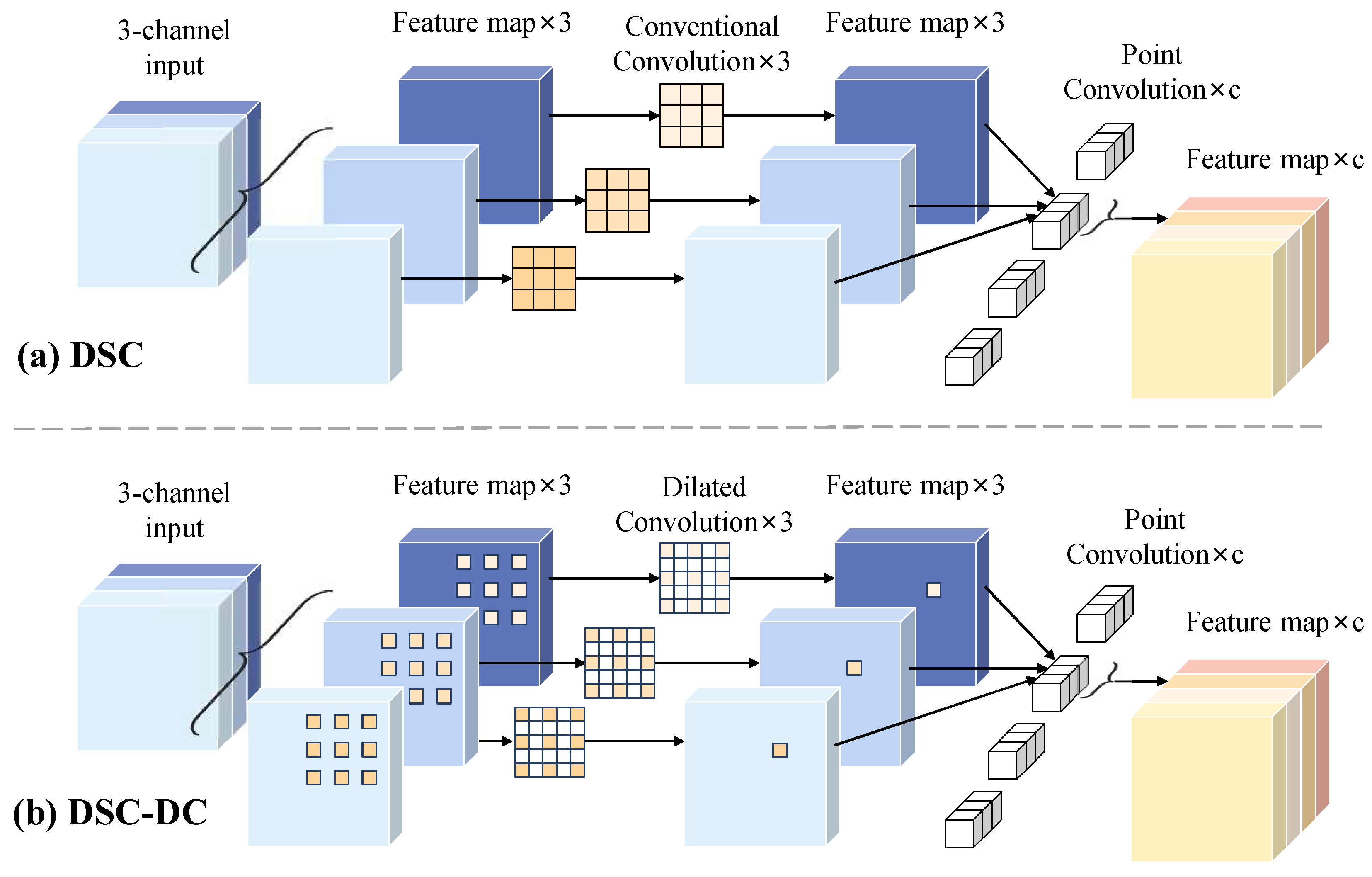
Figure 7.
The structures of DSC and DSC-DC, the parameter “c” represents the number of the output channels.
Figure 7.
The structures of DSC and DSC-DC, the parameter “c” represents the number of the output channels.
Figure 8.
Schematic of receptive field of the dilated convolution and conventional convolution. (a) The receptive fields of dilated convolution and conventional convolution. (b,c) Pixel coverage under different expansion rate groups.
Figure 8.
Schematic of receptive field of the dilated convolution and conventional convolution. (a) The receptive fields of dilated convolution and conventional convolution. (b,c) Pixel coverage under different expansion rate groups.
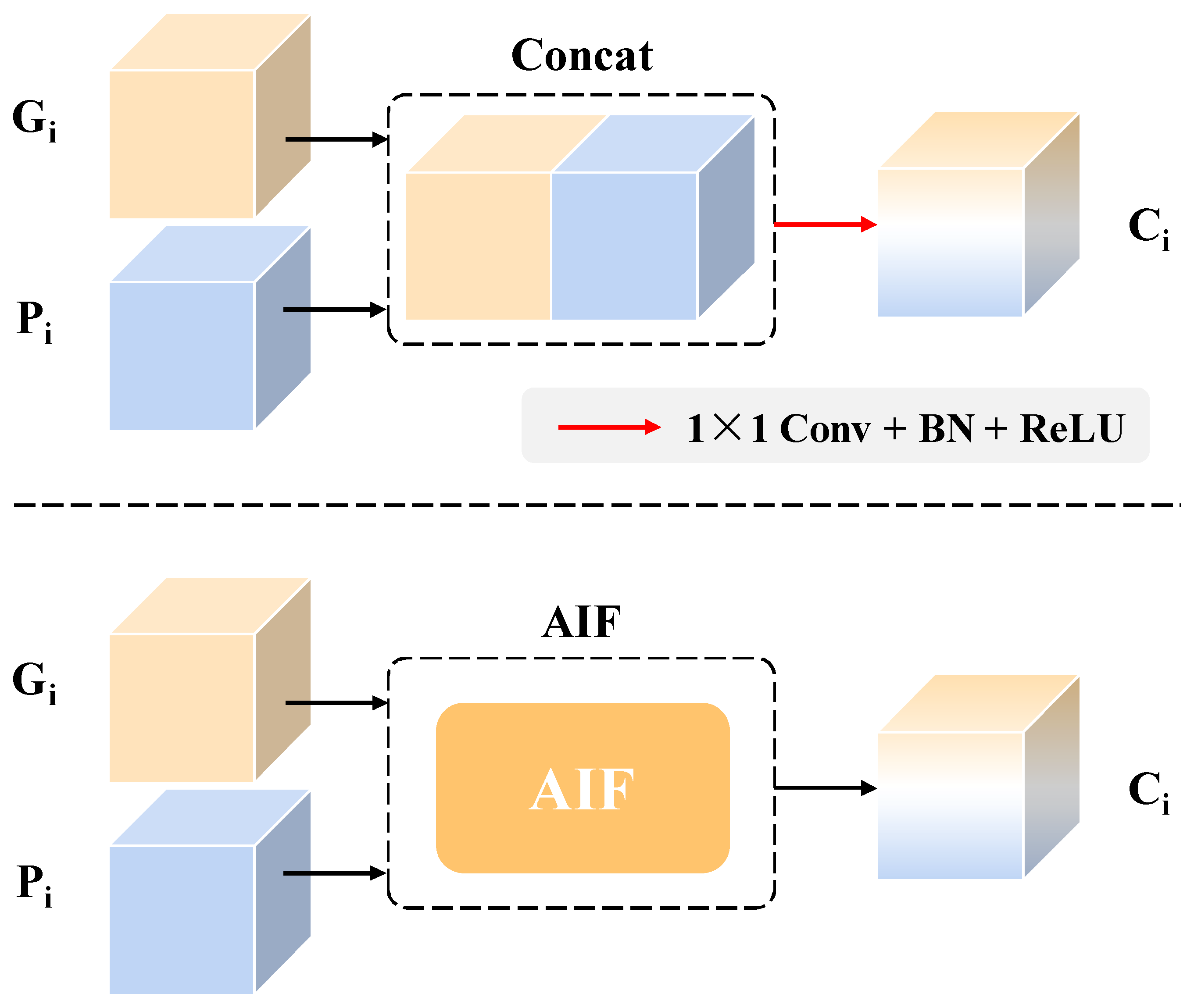
Figure 9.
The structure of the proposed adaptive interacting fusion (AIF) module.
Figure 9.
The structure of the proposed adaptive interacting fusion (AIF) module.
Figure 10.
The schematic of different input types.
Figure 10.
The schematic of different input types.
Figure 11.
Different fusion types between and . The upper type denotes the concatenation operation, and the lower type refers to our proposed method.
Figure 11.
Different fusion types between and . The upper type denotes the concatenation operation, and the lower type refers to our proposed method.
Figure 12.
Comparison of segmentation results. (a) Original image. (b) Original depth data. (c) Ground-truth. (d) U-Net with ResNet50. (e) U-Net with VGG16. (f) PSPNet with ResNet50. (g) PSPNet with MobileNetv2. (h) DeepLabv3 with MobileNetv2. (i) DeepLabv3 with Xception. (j) SegFormer with MiT-B0. (k) SegFormer with MiT-B1. (l) SegFormer with MiT-B2. (m) Ours.
Figure 13.
Analysis of failure cases. (a) Original image. (b) Original depth data. (c) Ground-truth. (d) Detection result.
Figure 13.
Analysis of failure cases. (a) Original image. (b) Original depth data. (c) Ground-truth. (d) Detection result.
Table 1.
The detail structure of the backbone.
Table 1.
The detail structure of the backbone.
| Backbone
| Type | Number | Output Size |
|---|
| Input | – | – | 512 × 512 × 1 |
| D-Conv1 & I-Conv1 | 7 × 7 Conv, 1s = 2 | 1 | 256 × 256 × 64 |
| 3 × 3 Max-pool, s = 2 | – | 128 × 128 × 64 |
| D-Conv2 & I-Conv2 | Res-DSC, 2c = 64 | 3 | 128 × 128 × 64 |
| 3 × 3 Max-pool, s = 2 | – | 64 × 64 × 64 |
| D-Conv3 & I-Conv3 | Res-DSC, c = 128 | 4 | 64 × 64 × 128 |
| 3 × 3 Max-pool, s = 2 | – | 32 × 32 × 128 |
| D-Conv4 & I-Conv4 | Res-DSC-DC, c = 256 | 2 | 32 × 32 × 256 |
| 3 × 3 Max-pool, s = 2 | – | 16 × 16 × 256 |
| D-Conv5 & I-Conv5 | Res-DSC-DC, c = 512 | 1 | 16 × 16 × 512 |
Table 2.
Experimental environment.
Table 2.
Experimental environment.
| Category | Version |
|---|
| GPU | Nvidia GTX 2060S (12 GB, 1470 MHz) (Nvidia, Clara, CA, USA) |
| CPU | Intel i5-12400F (2.5 GHz 4.4 GHz) (Intel, Clara, CA, USA) |
| Programming | Python 3.8.8 + Pytorch 1.10.0 + Cuda 102 |
| Operating system | Windows 11 × 64 |
Table 3.
Performance comparison of different backbones and different input types.
Table 3.
Performance comparison of different backbones and different input types.
| Input Types | U-Net Encoder | mIoU (%) | Acc (%) | mRec (%) | mPre (%) | mF1 (%) |
|---|
| Depth Data | ResNet18 | 69.06 | 97.97 | 82.06 | 78.20 | 80.08 |
| ResNet34 | 71.32 | 98.05 | 82.03 | 81.37 | 81.70 |
| ResNet50 | 70.65 | 97.97 | 84.06 | 78.67 | 81.28 |
| Image | ResNet18 | 76.85 | 98.53 | 88.56 | 84.01 | 86.23 |
| ResNet34 | 77.19 | 98.64 | 85.81 | 86.87 | 86.34 |
| ResNet50 | 76.52 | 98.53 | 87.99 | 83.97 | 85.94 |
1 Concat
data | ResNet18 | 76.79 | 98.60 | 85.59 | 86.51 | 86.05 |
| ResNet34 | 76.96 | 98.58 | 87.56 | 84.87 | 86.19 |
| ResNet50 | 76.13 | 98.65 | 83.46 | 88.60 | 85.95 |
Table 4.
The parameters and computational resources of different backbone.
Table 4.
The parameters and computational resources of different backbone.
| Backbone | Parameters (M) | FLOPs |
|---|
| ResNet18 | 11.17 | 0.93 × |
| ResNet34 | 21.28 | 1.90 × |
| ResNet50 | 23.50 | 2.12 × |
Table 5.
Ablation study of DSC and DC in the improved ResNet34.
Table 5.
Ablation study of DSC and DC in the improved ResNet34.
| ResNet34 | DSC | DC | mIoU | Acc | mRec | mPre | mF1 |
|---|
| √ | | | 76.96 | 98.58 | 87.56 | 84.87 | 86.19 |
| √ | √ | | 77.25 | 98.67 | 85.02 | 87.82 | 86.39 |
| √ | | √ | 77.32 | 98.58 | 89.40 | 83.78 | 86.50 |
| √ | √ | √ | 78.56 | 98.76 | 86.75 | 87.88 | 87.31 |
Table 6.
The parameters and computational resources of different backbone.
Table 6.
The parameters and computational resources of different backbone.
| Backbone | Parameters (M) | FLOPs |
|---|
| ResNet18 | 11.17 | 0.93 × |
| ResNet34 | 21.28 | 1.90 × |
| Improved ResNet34 (ours) | 10.00 | 0.94 × |
Table 7.
Performance comparison of different input data and different fusion types of and .
Table 7.
Performance comparison of different input data and different fusion types of and .
| U-Net Encoder | Data | Fusion Type | mIoU | Acc | mRec | mPre | mF1 |
|---|
Improved
ResNet34 | Depth | – | 72.35 | 98.19 | 85.02 | 81.84 | 83.40 |
| Image | – | 77.73 | 98.64 | 87.60 | 86.13 | 86.86 |
Depth
& Image | AIF (ours) | 79.73 | 98.85 | 87.38 | 88.86 | 88.11 |
| 1 Concat | 78.56 | 98.76 | 86.75 | 87.88 | 87.31 |
Table 8.
Performance comparison of different segmentation methods.
Table 8.
Performance comparison of different segmentation methods.
| Methods | Backbone | mIoU (%) | Acc (%) | mRec (%) | mPre (%) | mF1 (%) |
|---|
| U-Net | ResNet50 | 77.70 | 98.64 | 87.14 | 86.89 | 86.70 |
| U-Net | VGG16 | 77.84 | 98.74 | 84.82 | 89.57 | 86.79 |
| PSPNet | ResNet50 | 76.44 | 98.59 | 86.56 | 85.12 | 85.78 |
| PSPNet | MobileNetv2 | 73.61 | 98.36 | 84.62 | 82.78 | 83.68 |
| DeepLabv3 | MobileNetv2 | 75.86 | 98.59 | 84.87 | 85.87 | 85.36 |
| DeepLabv3 | Xception | 71.04 | 98.44 | 76.99 | 88.22 | 76.99 |
| Segformer | MiT-B0 | 78.91 | 98.71 | 89.02 | 86.38 | 87.55 |
| Segformer | MiT-B1 | 77.13 | 98.48 | 90.81 | 82.79 | 86.28 |
| Segformer | MiT-B2 | 76.98 | 98.52 | 88.66 | 84.27 | 86.17 |
| Ours | Improve ResNet34 | 79.73 | 98.85 | 87.38 | 88.86 | 88.11 |


