Abstract
Lateral flow immunoassay (LFIA) is extensively utilized for point-of-care testing due to its ease of operation, cost-effectiveness, and swift results. This study investigates the flow dynamics and reaction mechanisms in LFIA by developing a three-dimensional model using the Richards equation and porous media transport, and employing numerical simulations through the finite element method. The study delves into the transport and diffusion behaviors of each reaction component in both sandwich LFIA and competitive LFIA under non-uniform flow conditions. Additionally, the impact of various parameters (such as reporter particle concentration, initial capture probe concentrations for the T-line and C-line, and reaction rate constants) on LFIA performance is analyzed. The findings reveal that, in sandwich LFIA, optimizing parameters like increasing reporter particle concentration and initial capture probe concentration for the T-line, as well as adjusting reaction rate constants, can effectively enhance detection sensitivity and broaden the working range. Conversely, in competitive LFIA, the effects are inverse. This model offers valuable insights for the design and enhancement of LFIA assays.
1. Introduction
Lateral flow immunoassay (LFIA) has been widely used in recent years as a mainstream instant diagnostic method due to its advantages of easy operation, low material cost, and fast detection speed [1,2]. It has been widely applied in medical diagnosis, food safety, environmental monitoring, and other fields [3,4,5,6,7,8]. Large molecular analytes such as proteins are typically tested using sandwich assays, while small molecule analytes such as drugs of abuse are analyzed using competitive or inhibitory assays [9,10,11]. There may be multiple forms of reaction patterns, but they all have a common feature: reporter particles are captured by reagents immobilized on the test and control lines to form complexes, which generate visual signals within minutes. LFIA can easily obtain qualitative or semi-quantitative results, but compared to large quantitative detection instruments, it has many limitations in sensitivity.
Researchers have made many innovative efforts to improve the sensitivity of LFIA, such as inventing new reporter particles [12,13], optimizing membrane properties [14,15], improving experimental reagents [16,17], modifying LFIA geometry [18,19,20], and using different technologies [21,22,23]. These innovations have indeed enhanced the detection sensitivity. However, the development of lateral flow immunoassay test strips from the design stage to product development and final manufacturing is a process that applies principles of biology, chemistry, physics, and engineering. Structural and material changes require a considerable amount of experimentation [24].
In this context, computer simulation has become a practical tool to reduce the large amount of experimental work required for LFIA development. Simulation models of LFIA will allow developers to design and explore different architectures, materials, and analysis formats to seek better binding efficiency and improved detection sensitivity. Furthermore, running these simulation experiments significantly reduces development costs and time. Gasperino et al.’s review summarizes existing models [25], emphasizing the importance of computational models in quantifying performance and predicting future trends. Qian pioneered the establishment of mathematical models for sandwich and competitive LFIA [26,27], including a complete set of coupled reactions considering uniform and constant fluid velocity through the test lines. Berli proposed a simple mathematical model that condenses the main system parameters into two dimensionless parameters [28], relative fluid velocity, and relative analyte concentration, to quantitatively describe the dynamics of analyte capture in LFIA. Sotnikov used analytical (non-numerical) methods to calculate the dynamics of immune complex formation in continuous flow systems and also proposed an analysis of competitive LFIA under non-equilibrium conditions [29], obtaining symbolic solutions of differential equations describing the system [30]. Liu et al. established a model where reporter particles can bind to multiple target molecules and also developed a method to convert LFIA design parameters between simulation and experimentation [31,32]. Furthermore, they combined Langmuir surface reaction with convection–diffusion reaction equations to establish a thickness model for LFIA [33]. Asadi conducted a numerical study of spontaneous self-suction of shearing-related fluids using an improved Richards equation, showing that the average velocity of LFIA on the test line is strongly influenced by the microstructure of the absorption pad [34]. Schaumburg modeled LFIA using the finite element method in a Python environment and discussed its application in different dimensions [20].
Inspired by the work of Schaumburg and Liu, expanded on Qian’s numerical model and the COMSOL model established by Ed Fontes [35], we develop a 3D model of LFIA within the framework of porous media transport phenomena in COMSOL. Finite element simulations of sandwich LFIA and competitive LFIA were conducted to analyze a complete set of biochemical reactions involved in LFIA throughout the entire 3D domain. This included capillary-driven flow velocities, transport and diffusion of each reaction component under non-uniform flow, and the effects of different parameters (analyte concentration, reporter particle concentration, initial capture probe concentrations for T-line and C-line, reaction rate constants) on LFIA performance.
2. Mathematical Modeling
In this section, we use equations to simulate all the transport phenomena related to the performance of LFIA, including fluid dynamics, solute transport, and reaction kinetics. The model is based on the classical approach of porous media, where the microstructural properties of the matrix are represented by macroscopic parameters such as porosity, pore size, and permeability.
2.1. Fluid Dynamics Model
The lateral flow immunoassay strip is a porous structure, and the interaction between the liquid and the pore walls causes capillary forces that drive the liquid forward. In this paper, the Richards equation is used to describe the fluid dynamics model of capillary seepage in porous media. The Richards equation is primarily used to analyze flow in variably saturated porous media. In this type of flow, as the fluid passes through the porous medium, it fills some pores and drains from others, leading to changes in hydraulic properties. The specific expression is as follows:
In the equation, is the density of the solution; is the effective saturation; is the specific storage coefficient; is the specific moisture capacity; is the pore water pressure; g is the acceleration due to gravity; is the Hamiltonian operator; is the flow velocity; is the sink or source term of the solution; is the porosity; is the saturation volumetric fraction; is the dynamic viscosity; is the permeability; is the saturated hydraulic conductivity; and is the relative hydraulic conductivity. The parameters related to unsaturated seepage in this model are all fitted using the Brooks–Corey model.
2.2. Transport of Dilute Species in Porous Media
The transfer of dilute species in porous media is mainly used to simulate the migration and reaction of substances in porous media, calculating the concentration and transfer of substances in porous media, including the transfer mechanisms of diffusion, convection, migration, dispersion, adsorption, and volatilization of chemical substances in porous media. The specific expression is as follows:
In the formula, is the volumetric water content; is the density of the solution; is the solute concentration in the solution; is the adsorbed concentration in the solution; is the concentration of reaction products; is the liquid volume fraction; is the Hamiltonian operator; is the diffusion term of the equation, is the diffusion flux, where , is the dispersion tensor; is the effective diffusion coefficient; is the dynamic viscosity; is the convective term of the equation; is the reaction term; is the sink or source term of the solution.
2.3. Reaction Kinetics Model
In the following sections, we will focus on the formulation of numerical prototypes for antigen–antibody reactions. These models are based on the following assumptions [26,27,28,29,30]:
- Antigens consist of single molecules and exist in homogeneous form, as do antibodies.
- One report particle combines one target analyte.
- Binding is consistent, without positive or negative allosteric effects (binding of one site on the analytes does not affect the binding of another site to the antibody).
- The reaction is a first-order reversible interaction, with concentrations of reactants reaching a steady state over time.
- There is no non-specific binding, such as binding to the reaction vessel walls.
- The rate constants of the reaction are constant, meaning they do not change with variations in reagent and sample concentrations during the reaction process.
2.3.1. Sandwich LFIA Reaction Kinetics Model
The components of the model are represented as follows:
—Analytes;
—Reporter particle;
—Complex formed by analytes and reporter particle;
—Capture probe, immobilized on the test line;
—Complex formed by analytes captured by the test line;
—Complex formed by analytes, reporter particle, and antibody immobilized on the test line;
—Capture probe, immobilized on the control line;
—Complex formed by free reporter particle captured by the control line;
—Complex formed by analytes, reporter particle, and antibody immobilized on the control line.
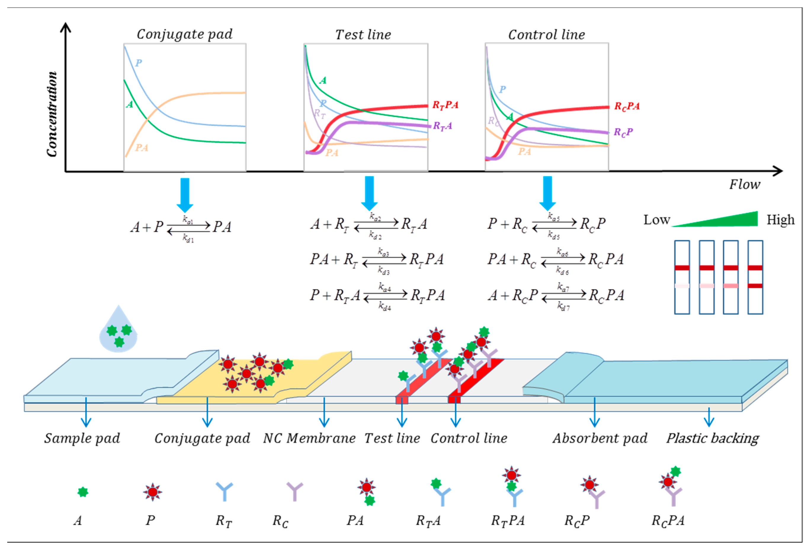
In the Sandwich LFIA reaction process and equations as depicted in Figure 1, the sample liquid is dispensed onto the sample pad, and due to capillary action, it migrates forward. The analytes () in the sample liquid reacts with the reporter particles () on the conjugate pad to form the analyte–reporter particle complex () upon passing through the conjugate pad. When the mixture of (), (), and () migrates to the test line (T-line), the capture antibody () on the test line captures the analytes () and the analyte–reporter particle complex (), forming () and (), respectively. The complex () may further interact with free reporter particles () to form (). At the control line, the reporter particles () and () are captured by the control line antibody () to form () and (), respectively. The complex () may further interact with free analytes () to form (). These biochemical reactions are reversible, where represent the association rate constants, and represent the dissociation rate constants.

Figure 1.
Schematic diagram of the sandwich LFIA model and reaction processes. The model depicts all the reaction processes involved in LFIA.
During the reaction process, the concentrations of each substance can be considered as a function of the position x on the lateral flow strip and the reaction time t. They all satisfy the convection–diffusion equation and fluid dynamics equations. Solving these partial differential equations for the concentration functions of each substance at any position and time during the reaction process yields the concentration profiles. For ease of understanding, we represent each substance involved in the reaction with the letters or combinations of letters enclosed in parentheses. denote the concentrations of the respective substances, with subscript 0 indicating the initial concentrations.
According to material conservation and reaction kinetics equilibrium, the reaction rates for each component are calculated as follows [26]:
The reaction rate constants for the analyte–antibody interaction are adopted from Qian [26], where and .
The diffusion–reaction equations for all species are as follows:
where is the concentration of the species, is the diffusion coefficient, is the fluid velocity, and is the reaction rate of species i. The complete set of equations for each species is listed as follows [26]:
where and are the diffusion coefficients for the analytes () and the complex of analytes and reporter particles (), respectively [26].
2.3.2. Competitive LFIA Reaction Kinetics Model
The commonly observed reaction mode in commercially available competitive LFIA involves the competition between the capture probe on the T-line and the antibody conjugated to the reporter particles for the target analytes. This study exclusively analyzes this competitive reaction model.
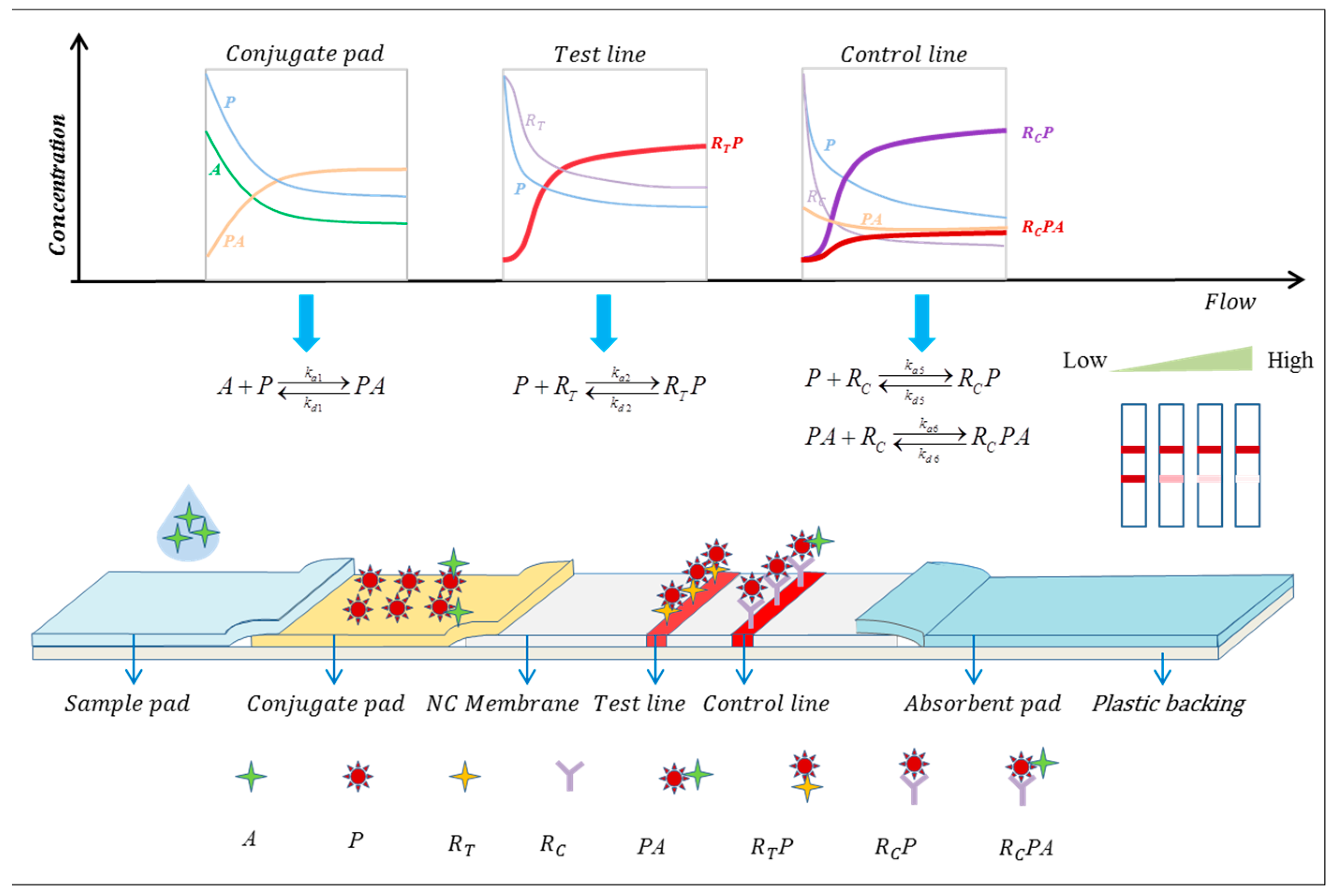
The competitive LFIA reaction process and equations are shown in Figure 2. After the sample liquid is dropped onto the sample pad, due to the capillary action, the analytes () in the sample liquid reacts with the reporter particles () on the conjugate pad to form the analyte–reporter particle complex () when passing through the conjugate pad. When the mixture of (), (), and () migrates to the test line, the antigen analogue () on the test line captures the free reporter particles () to form (). At the control line, the reporter particles () and () are captured by the control line antibodies () to form () and (), respectively. These biochemical reactions are reversible, where represents the association rate constants, and represents the dissociation rate constants.
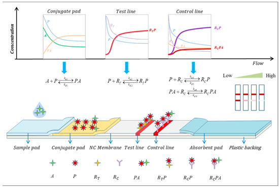
Figure 2.
Schematic diagram of the competitive LFIA model and reaction processes. The model depicts all the reaction processes involved in LFIA.
Assuming no time delay in the four biochemical reaction processes, the rates of the four biochemical reactions are given by [27]:
From the convection–diffusion equations, we can obtain:
3. Finite Element Simulation
3.1. Simulation Approach
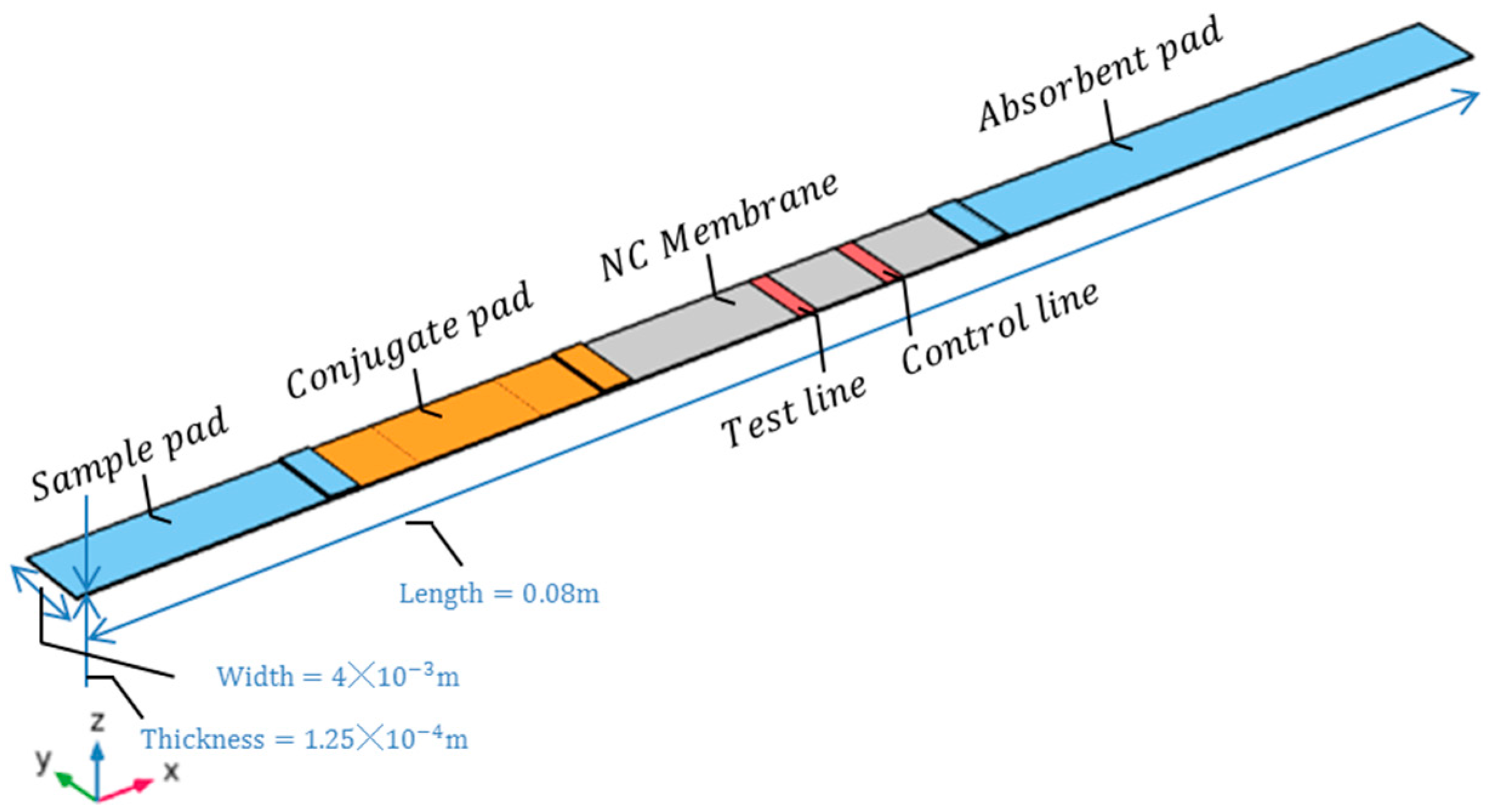
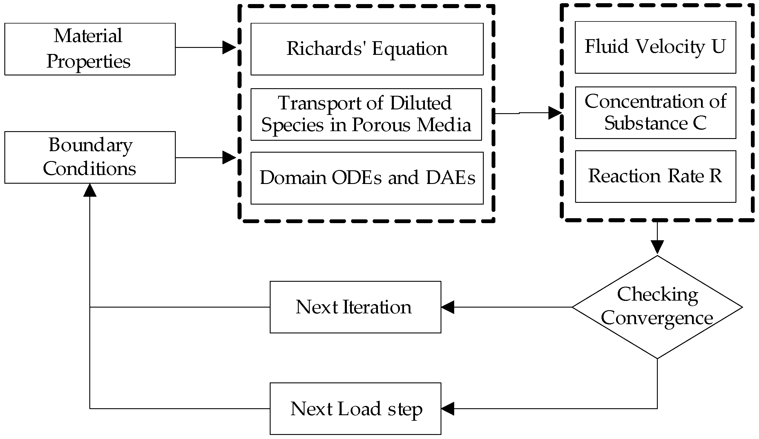
In COMSOL, LFIA three-dimensional models were established using the Richards equation, transport of dilute species in porous media, and domain ordinary differential equation physics interfaces, and the geometric diagram of the model is shown in Figure 3. The simulation process involves iterative calculations of fluid velocity, substance concentration distribution, and reaction rate coupling fields. During the solving process, COMSOL utilizes iterative algorithms to gradually approximate the solution of the model, as illustrated in Figure 4.
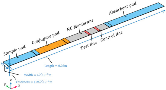
Figure 3.
Schematic diagram of the 3D geometry model of LFIA.
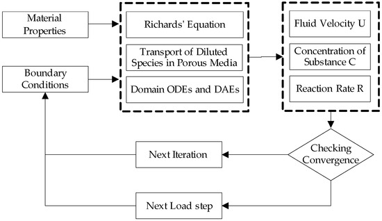
Figure 4.
Flowchart of the solution scheme for LFIA simulation.
Set material properties and initial conditions for the model, including porous media and fluid. Specifically, materials such as NC membrane and other components (sample pad, conjugate pad, absorbent pad) are set as porous materials with different parameters (porosity, pore size, permeability, etc.), as detailed in Table 1. The initial conditions of the model include the initial concentration distribution of various substances, the initial state of the porous media, and the initial conditions of the domain, as described in Section 3.2. Select the solver and iterative algorithm to start iterative calculations. In each iteration, COMSOL updates boundary conditions based on the current solution and adjusts them according to residuals or other convergence criteria. Using the updated boundary conditions, the solver is called again, gradually approaching the final solution. This iteration scheme is repeated until the fluid velocity becomes zero, but the reaction–diffusion process continues to evolve. The solver continues to iterate until the final time step is reached.

Table 1.
Main model parameters.
3.2. Model Parameter Settings, Initial Conditions, and Boundary Conditions
Set model parameters, including geometric parameters, porous material parameters, physical parameters of the Richards equation and initial concentrations of each substance. The main model parameters include the following:
Using the Richards equation to model liquid-phase transport in porous media, the following are defined:
No-flow boundary:
Initial pressure value:
Sample pad as fluid inlet, pressure head:
The solving substance concentration and reaction rate are determined using the transport of dilute species in porous media and domain ODEs and DAEs interfaces. Fluid velocity is determined by the Richards equation, selecting the corresponding reaction region, setting the initial substance concentration as:
Initial concentration of other substances is set to 0.
The sample pad is set as the inlet, with the inlet boundary condition:
The absorbent pad is the outlet, with the outlet boundary condition:
The reaction rate of each substance in the corresponding reaction region is set, with the sandwich LFIA according to Equations (5)–(13) and the competitive LFIA according to Equations (22)–(25).
3.3. Parameter Definitions
When the computing system reaches equilibrium, the detection signal is obtained at 600 s. Theoretically, the concentration of the composite particles captured on the test line and control line is proportional to the available detection signal (optical signal, magnetic signal) in experiments. Therefore, in this study, the volume-averaged concentrations of the composite particles captured on the T-line and C-line are defined as the T-line and C-line analysis signals:
Sandwich LFIA:
where V is the volume of the T-line or C-line.
In sandwich LFIA, we take 1.5 × 10⁻⁹ M as the threshold value STL for ST. The target analyte concentration (CAL) corresponding to the threshold value STL is defined as the detection limit (CAL). The range of target analyte concentrations (CAM) corresponding to the maximum signal (STmax) from the detection limit (CAL) to ST is defined as the working range (WR) [32]:
Competitive LFIA:
In Competitive LFIA, the detection limit for competitive LFIA is chosen as IC10, and the working range is IC20–IC80.
4. Results and discussion
4.1. The Effect of Flow Velocity on LFIA Performance
Flow velocity is one of the most important factors affecting the sensitivity of LFIA. In LFIA, once the analytes and reporter particles in the sample solution pass through the T-line and C-line, they cannot be captured. A slower flow velocity allows more interactions between reporter particles and capture reagents, leading to higher signal intensity [36]. Flow velocity is difficult to measure accurately in experiments, but it can be easily calculated in finite element simulation software.
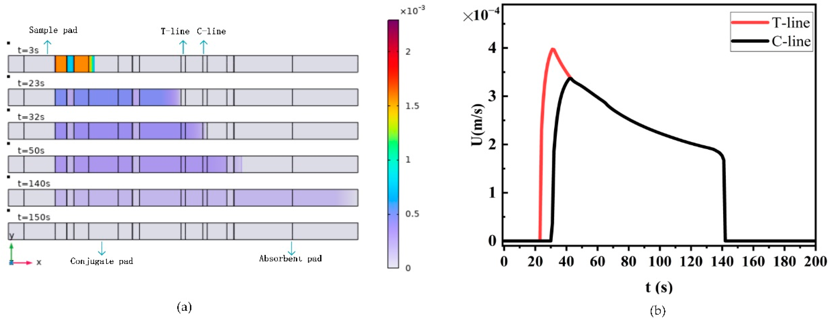
We simulated the flow velocity on the test strip using the Richards equation (Figure 5). The distribution of sample liquid flow velocity at different times on the test strip is shown in Figure 5a. The sample solution reaches the binding pad, T-line, C-line, and absorption pad at 3 s, 23 s, 32 s, and 50 s, respectively, and fills the entire test strip by 140 s, with the flow velocity rapidly decreasing to 0.

Figure 5.
Sample liquid flow velocity figure. (a) Sample flow velocity contour plot; (b) flow velocity plot at T-line and C-line positions.
For comparison, we extracted the flow velocity profiles at the T-line and C-line (Figure 5b). It can be observed that the sample flow velocity decreases almost exponentially as the distance of the liquid front from the origin increases. This is because the capillary forces driving liquid flow only acts on the surface of the porous material where the sample solution meets the air (the three-phase boundary region of the liquid front). This means that the capillary force is constant, and as long as there is free pore volume, it can be filled with the sample solution. However, as the sample solution further enters the test strip, the flow resistance increases, leading to a decrease in flow velocity. The trend of the results calculated by the model is consistent with the trend derived by Mendez [37] based on the Lucas–Washburn equation.
The flow velocity of the membrane mainly depends on the properties of the porous structure, including pore size and porosity, and discussing these parameters helps us to understand capillary flow. Flow velocity is difficult to measure accurately in experiments, so commercial NC membranes typically use a parameter called capillary flow time (CFT) to reflect capillary flow velocity—the time required for the liquid to move along a specified length of strip and completely fill it. The larger the CFT value, the slower the capillary flow. We compared the flow velocities of liquids with different pore sizes and porosities passing through the T-line, and extracted the time and average velocity at which the liquid passes through the T-line (Figure 6).
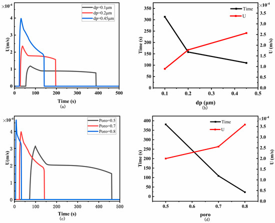
Figure 6.
Effect of different pore sizes and porosities on flow velocity. (a) Flow velocity of liquid passing through the T-line for different pore sizes; (b) time and average velocity of liquid passing through the T-line for different pore sizes; (c) flow velocity of liquid passing through the T-line for different porosities; (d) time and average velocity of liquid passing through the T-line for different porosities.
Pore size is a measure of the maximum pore diameter. In the simulated experiments, we compared three common pore sizes (dp = 0.1, 0.2, 0.45 μm) found in the market and plotted the flow velocity of the liquid passing through the T-line at different pore sizes (Figure 6a). From the graph, it can be observed that as the pore size increases, the membrane’s flow velocity also increases. For easier observation, we extracted the time taken for the liquid to flow through the T-line from Figure 6a and calculated its average velocity (Figure 6b). It is evident that with an increase in pore size, the flow velocity of the membrane increases, and the time taken for the liquid to flow through the T-line decreases.
Porosity is the volume of air in a three-dimensional membrane–membrane structure, usually expressed as a percentage of the total membrane volume. Porosity is typically unrelated to pore size and is not controlled by pore size. These two parameters are essentially independent. In the simulation, we set the porosity to 0.5, 0.7, and 0.8, and compared the flow velocity of the liquid passing through the T-line (Figure 6c). It can be observed that under the same conditions, the capillary flow velocity increases with an increase in porosity, and at the same time, the time taken for the liquid to flow through the T-line decreases (Figure 6d). When the porosity is set to 0.7, the simulated flow velocity of the liquid through the T-line is 0.00025 m/s, which is close to the average flow velocity of 0.0002 m/s measured in the experiments by Qian [26,27] and Liu [31]. This validates the accuracy of the model.
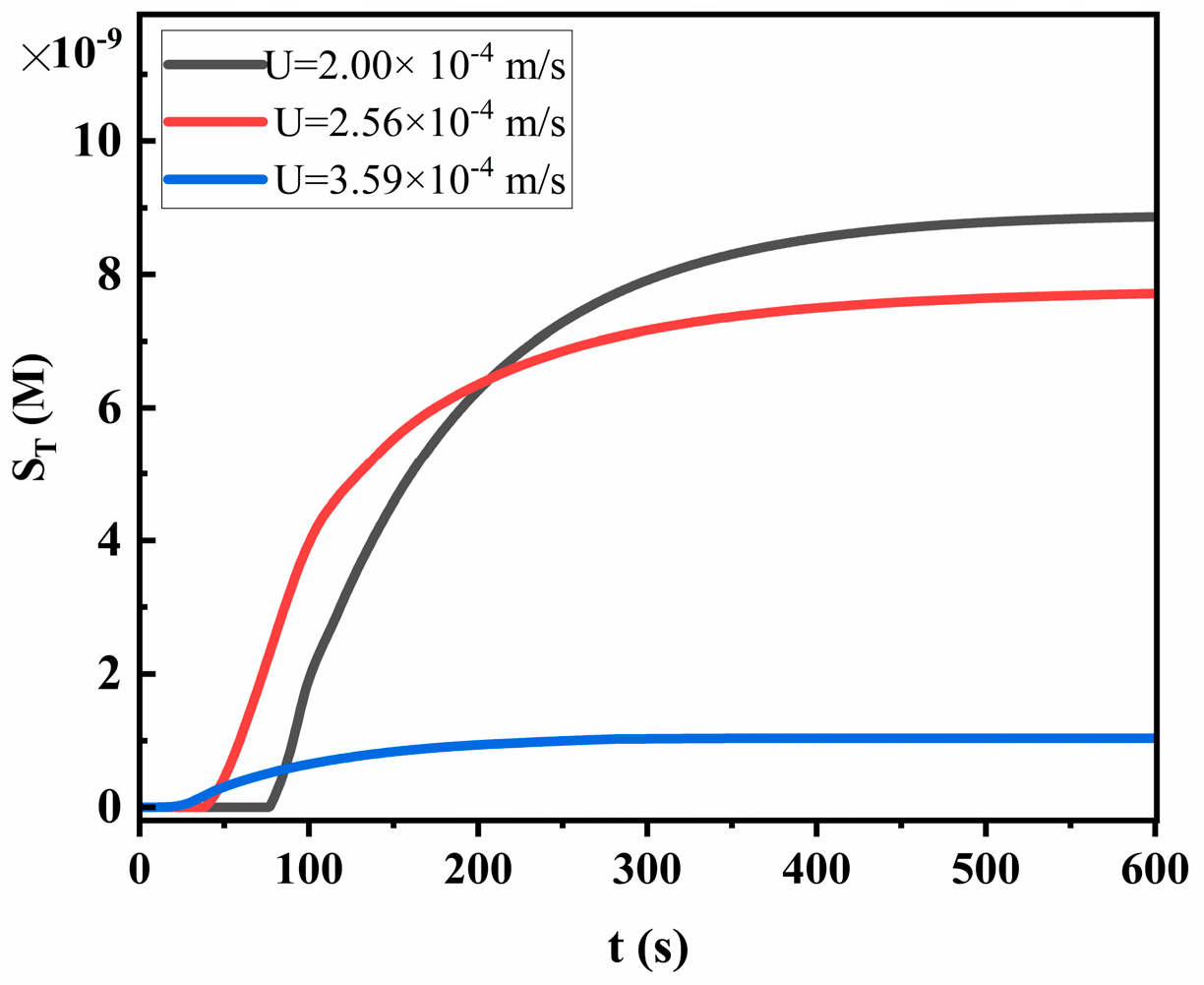
For a better observation of the impact of flow velocity on LFIA performance, we compared the variation trend of ST (taking competitive LFIA as an example) under different average flow velocities (Figure 7). As the flow velocity increases, the time for the liquid to flow on the T-line decreases, shortening the time for the reactants to come close enough to bind, significantly reducing ST and system sensitivity. This is why membranes with the fastest capillary flow are usually not used. The longer the reaction duration in the T-line and C-line, the higher the detection sensitivity and signal intensity of the T-line and C-line. Therefore, to achieve better analytical characteristics, the fluid front must pass through the T-line and C-line as slowly as possible. The structure of the NC membrane can be appropriately optimized (by selecting smaller pore size and lower porosity) or the viscosity of the sample can be increased to achieve this effect.
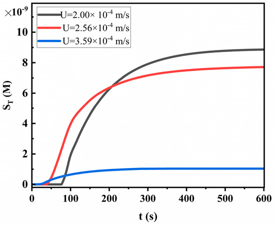
Figure 7.
The trend of ST under different flow velocities.
4.2. Sandwich LFIA
4.2.1. Sandwich LFIA Reaction Process
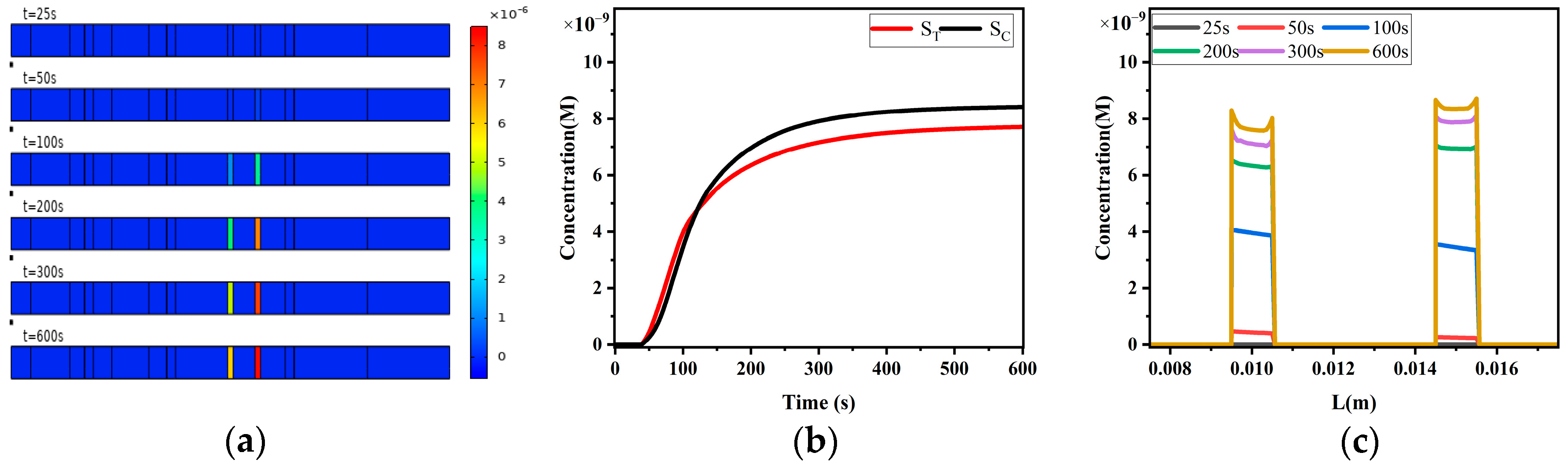
In this section, we explore the reaction process of the sandwich LFIA under the non-uniform flow conditions calculated in the previous section. The model assumes that each reaction component is uniformly distributed throughout the thickness of the entire test strip, and here, the model’s top view is used to represent the calculation results. Figure 8 shows the concentration distribution of analytes A (Figure 8a), reporter particles P (Figure 8b), analyte–reporter particle complex PA (Figure 8c), complexes RTPA, RCPA, RCP formed by capturing reporter particles on the T-line and capturing PA and reporter particles P on the C-line (Figure 8d) at different times.
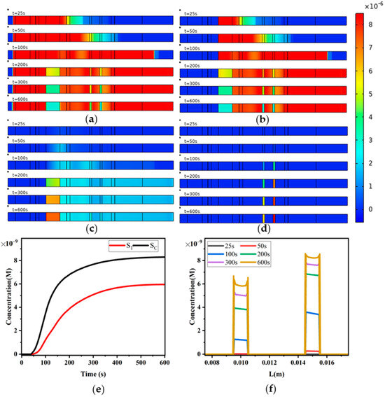
Figure 8.
Sandwich LFIA reaction process. (a) Concentration distribution map of analytes A; (b) concentration distribution map of reporting particles P; (c) concentration distribution map of complex PA formed by reporting particles and analytes; (d) concentration distribution map of reporting particle complexes captured by T-line and C-line; (e) variation in signals ST and SC over time for T-line and C-line; (f) diffusion effects of reporting particle complexes captured by T-line and C-line.
From Figure 8a, it can be observed that the analytes A, under the influence of capillary forces, exhibit lower concentration at the leading edge of the liquid flow. As it flows towards the right end of the absorbent pad, analytes A fill the entire test strip. A is consumed in the reaction zones including the binding pad, T-line, and C-line, leading to a decrease in concentration, while it is almost uniformly distributed elsewhere on the strip. The concentration distribution of reporting particles P (Figure 8b) is similar to that of the analytes A concentration distribution.
In Figure 8c, it can be seen that the complex PA travels with the liquid flow until it reaches the regions of T-line and C-line. Here, it reacts with the capture probes RT and RC on the T-line and C-line, respectively, forming colored detection lines (Figure 8d).
To further facilitate the observation of the reaction process at T-line and C-line, we analyzed the variation in ST and SC over time (Figure 8e). When the sample liquid reaches the T-line and C-line, particle concentrations begin to increase. As PA is captured in the regions of T-line and C-line, forming detection materials RTPA and RCPA, ST and SC exhibit nearly linear growth. When the absorbent pad saturates and flow stops, the growth in concentration slows down, indicating that under this condition, the formation of RTPA and RCPA is controlled by mass transport. Figure 8f displays the concentration distribution of the generated species along the x-direction on the surfaces of T-line and C-line, showing edge effects. The concentration is higher near x = 0, which can be easily explained as this edge is closest to the inlet where reactants are first captured. At the edge near the outlet, the concentration also increases due to diffusion effects, and this effect is also present at the edge positions near the inlet.
4.2.2. The Influence of Target Analyte Concentration on ST and SC in Sandwich LFIA
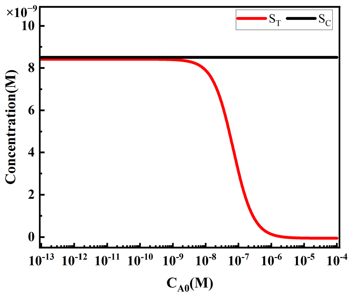
Figure 9 depicts the variation in ST and SC with the concentration of analytes A. When the concentration of the target analytes is very low, ST remains nearly constant. As the concentration of the target analytes increases, ST almost linearly increases as a function of CA0. With further increase in the concentration of the target analytes, ST reaches its maximum value at the concentration CAM of the target analytes, and then decreases. CAM corresponds to the concentration of the target analytes at the peak of ST, a phenomenon known as the “HOOK effect”, which is described in many literature sources. At high concentrations, the decrease in ST is due to the binding of analytes to reporting particles and capture probes, which hinders the binding of complex PA to RT. SC remains almost constant as the concentration of analytes changes, indicating that the concentration of analytes does not affect SC.
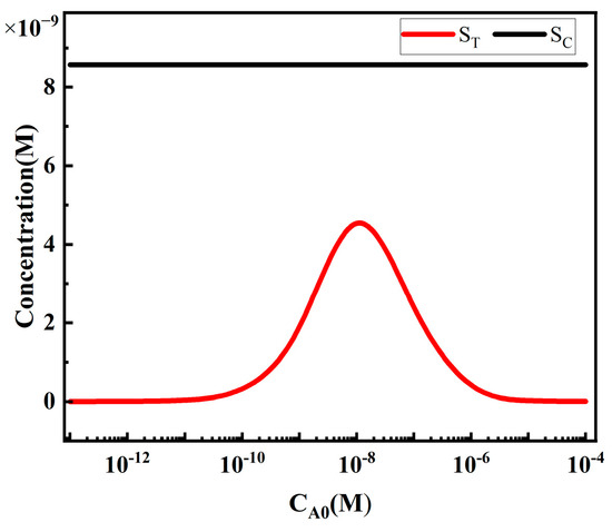
Figure 9.
The variation in ST and SC with the concentration of analytes.
4.2.3. The Influence of Reporter Particle Concentration on Sandwich LFIA Performance
The concentration of reporter particles P plays a significant role in the sensitivity of LFIA. We first investigated the effect of reporter particle concentration on the performance of sandwich LFIA (Figure 10).
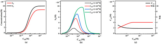
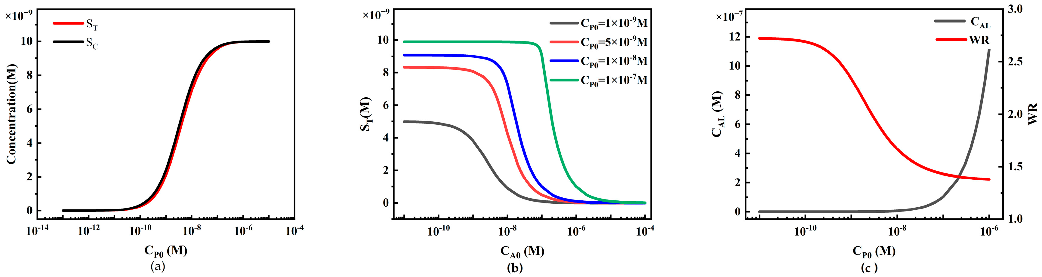
Figure 10.
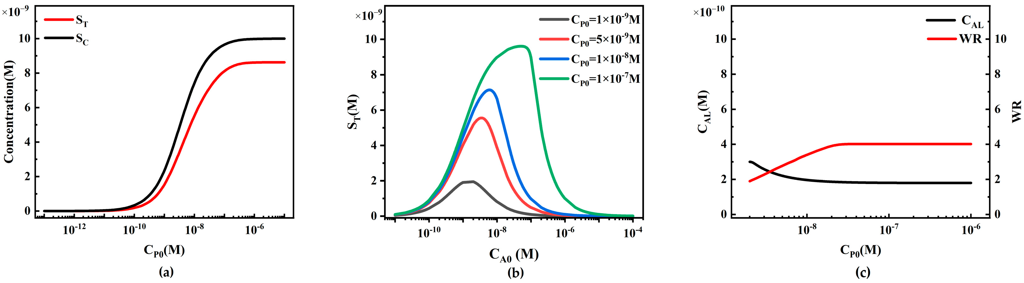
The relationship between reporter particle concentration and LFIA detection performance. (a) Variation in ST and SC with different reporter particle concentrations; (b) standard curves of the HOOK effect under different reporter particle concentrations; (c) trends of LFIA detection limit (CAL) and working range (WR) under different reporter particle concentrations.
When the analyte concentration remains constant, an increase in the concentration of reporter particles P positively affects the signal intensity on the T-line and C-line (Figure 10a). The simulation results show that at low concentrations, CP0 is low, and may not sufficiently cover the binding sites on the test and control lines, resulting in relatively constant concentrations of ST and SC. As CP0 concentration increases, more binding sites are occupied, and the concentrations of ST and SC begin to increase almost linearly. However, when CP0 concentration further increases to a certain extent, the binding sites on the test and control lines may become saturated, leading to a slowing down of the rate of increase in concentrations of ST and SC, showing a saturation state.
We also plotted standard curves of the HOOK effect for different CP0 values (1 × 10⁻⁹, 5 × 10⁻⁹, 1 × 10⁻⁸, and 1 × 10⁻⁷ M) (Figure 10b). The increase in initial concentration of reporter particles not only enhances the ST value corresponding to the peaks in the standard curve, but also results in a rightward shift in the peak in the HOOK effect standard curve. The rightward shift indicates an increase in the working range, possibly due to the increased strength of binding between reporter particles and analytes.
To further compare LFIA performance, we extracted the detection limit (CAL) and working range (WR) from the simulation results (Figure 10c). With the increase in CP0, the CAL in the simulation shows a decreasing trend (black line in Figure 10c), indicating that higher CP0 enhances system sensitivity. However, due to the limited capture capacity of the capture probes fixed on the T-line and C-line, this decreasing trend gradually becomes moderate. Additionally, it can be observed from the simulation results that as CP0 increases, the WR widens (red line in Figure 10c), indicating that appropriately increasing CP0 is beneficial for expanding the linear working range. The simulation results also reveal that the slopes of the CAL and WR curves gradually decrease, indicating that the capture capacity of the capture reagents on the T-line and C-line gradually saturates, and cannot bind more reporter particles. This model can be utilized to predict the standard curves, CAL, and WR under different CP0 values, assisting experimenters in selecting the optimal CP0 for LFIA with the best performance.
4.2.4. The Influence of Initial Capture Probe Concentration on Sandwich LFIA Performance
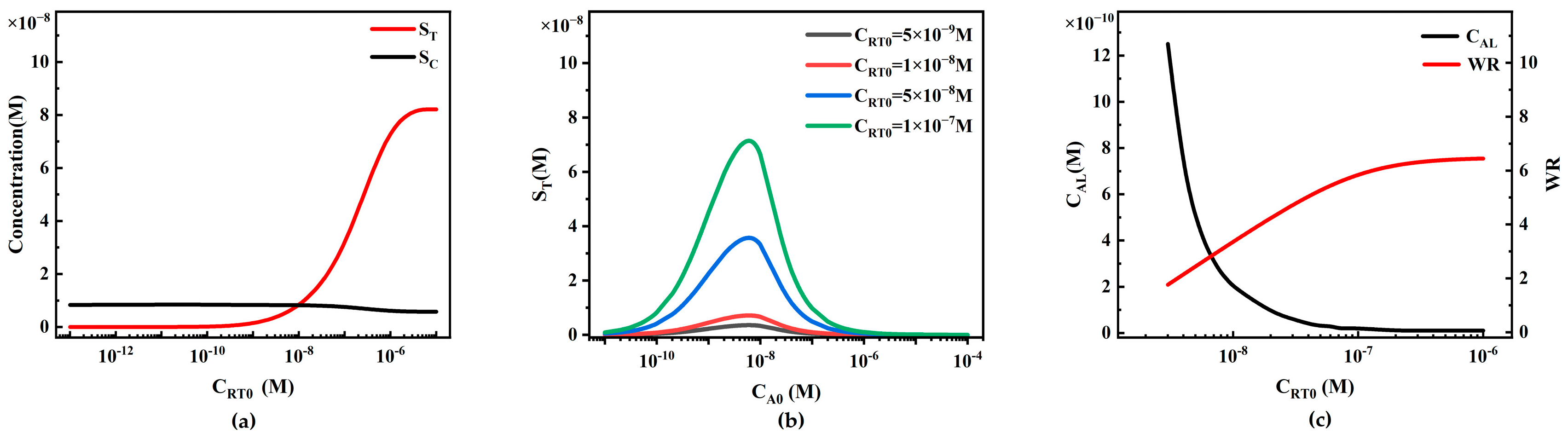
The initial concentration of capture probe CRT0 on the T-line is also a crucial parameter when preparing LFIA, and we investigated its impact on LFIA performance by calculating different concentrations of CRT0 (Figure 11).
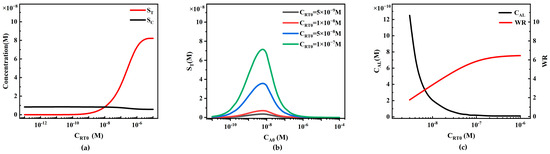
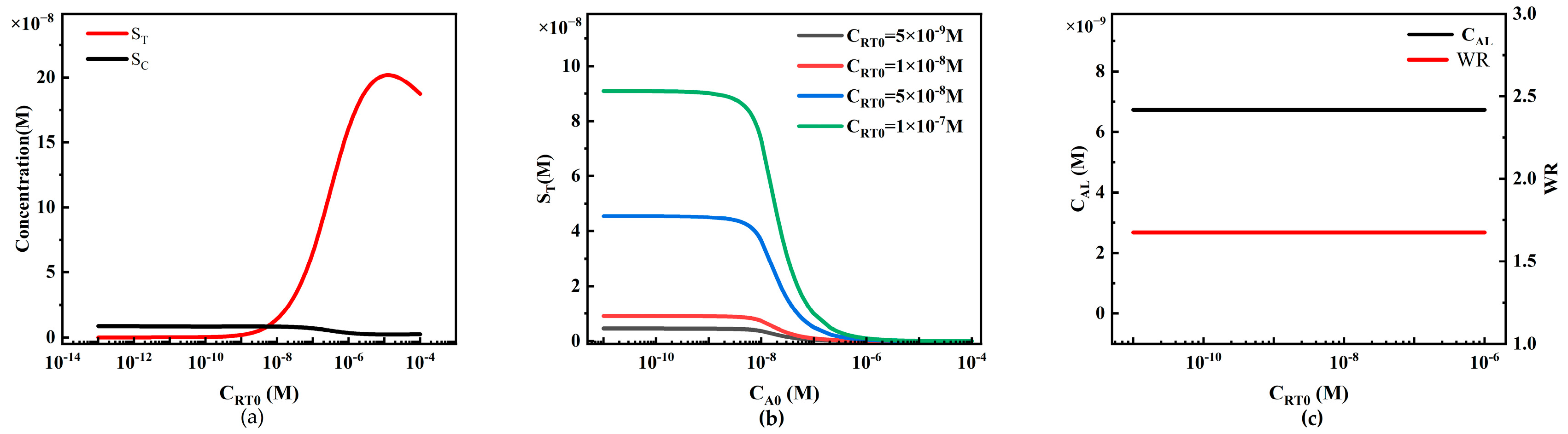
Figure 11.
The relationship between the initial capture probe concentration on the T-line and LFIA detection performance. (a) Variations in ST and SC with different initial capture probe concentrations on the T-line; (b) standard curves of the HOOK effect under different initial capture probe concentrations on the T-line; (c) trends of LFIA detection limit (CAL) and working range (WR) under different initial capture probe concentrations on the T-line.
When other conditions remain constant, CRT0 only affects ST, with little influence on SC (Figure 11a). When CRT0 is low, the effective capture of reporter particles and analytes is insufficient, resulting in a low and relatively constant ST. As the concentration of capture antibodies increases, the capture capacity increases, leading to an almost linear increase in ST. However, when the binding sites of the capture antibodies reach saturation (due to the limitation of CP0, preventing further binding of more reporter particles), even with further increases in the concentration of capture antibodies, ST cannot be further increased, reaching a saturation state. In the range of CRT0 = 1 × 10⁻⁸ to 1 × 10⁻⁶ M, when ST increases almost linearly, more reporter particles P are captured on the T-line, resulting in a decrease in reporter particles P on the downstream C-line, thus reducing SC.
We plotted concentration curves of ST at different analyte concentrations using different CRT0 values (5 × 10⁻⁹, 1 × 10⁻⁸, 5 × 10⁻⁸, and 1 × 10⁻⁷ M) (Figure 11b). The increase in CRT0 enhances the capture capacity of the T-line, enlarging the peak of the ST curve, significantly reducing the detection limit. As CRT0 increases, the CAL in the simulation shows a decreasing trend (black line in Figure 11c), indicating that higher CRT0 also increases sensitivity. However, as CRT0 increases, this decreasing trend gradually becomes less sensitive. The changes in the detection limit with different CRT0 are more pronounced compared to different CP0. Additionally, the WR in the simulation shows an expanding trend with the increase in capture probe concentration (red line in Figure 11c). Therefore, increasing CRT0 should be considered to lower the system detection limit and expand the system detection range. Similarly, this model can be used to predict standard curves, CAL, and WR under different CRT0 values, helping experimenters select the optimal CRT0 for LFIA with the best performance.
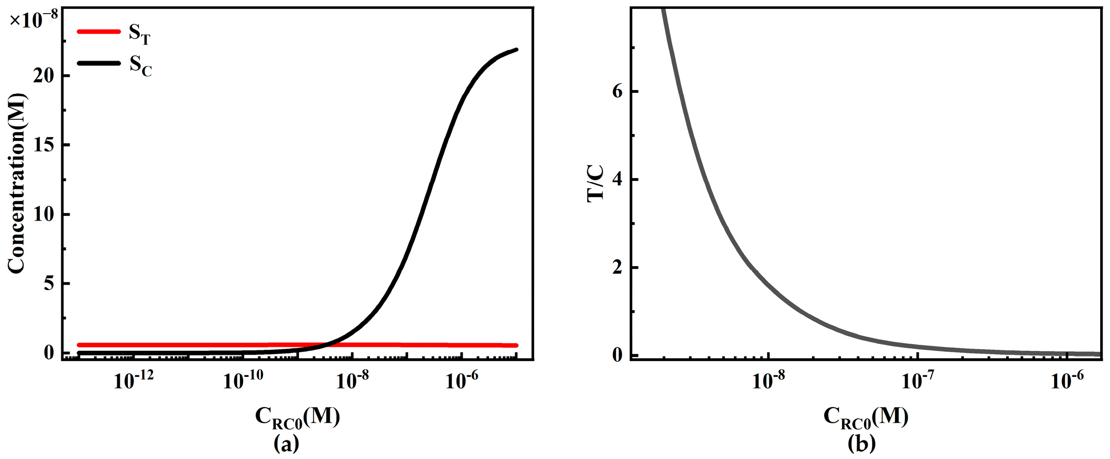
We also studied the influence of the initial concentration of capture probe CRC0 on LFIA performance (Figure 12). Theoretically, CRC0 only affects SC, with little influence on ST (Figure 12a). When CRC0 is low, the effective capture of reporter particles and analyte–reporter particle complexes is insufficient, resulting in a low and relatively constant SC. As the concentration of capture antibodies increases, the capture capacity increases, leading to an almost linear increase in SC. However, as CRC0 continues to increase, the trend of an increase in SC slows down due to the limitation of CP0, preventing further binding of more reporter particles.
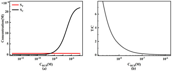
Figure 12.
The relationship between the initial capture probe concentration of the C-line and the LFIA detection performance. (a) The variation in ST and SC under different initial capture probe concentrations of the C-line; (b) the trend of T/C under different initial capture probe concentrations of the C-line.
Because ST is insensitive to changes in CRC0, similarly, the system detection limit and working range are also insensitive to changes in CRC0. However, in commercial quantitative detection, to reduce inter-batch variability, the T/C value is usually used as the final detection signal. When SC increases linearly with CRC0, the T/C value (ST/SC) decreases (Figure 12b). In practical detection, this change may lead to a decrease in detection sensitivity due to the influence of detection noise. Therefore, in experiments, CRC0 should be limited to avoid adversely affecting the system detection performance by keeping the T/C value from being too low.
4.2.5. The Influence of Reaction Rate Constants on Sandwich LFIA Performance
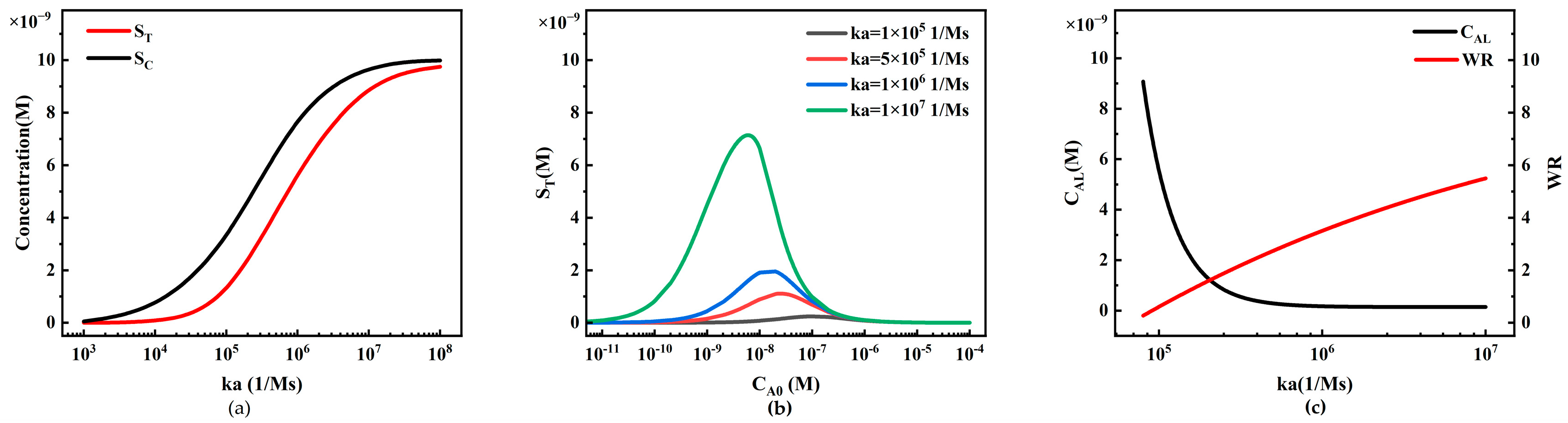
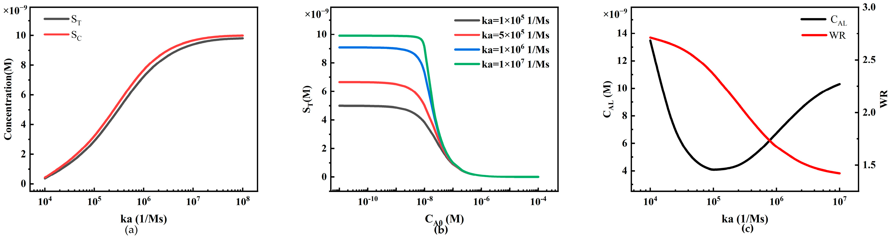
The reaction rate constants, including the association rate constant ka and the dissociation rate constant kd, play a crucial role in LFIA performance. Significant effort is required in experimental research to select antibodies with different ka and kd values because different ka and kd values correspond to different reagent reactions in various LFIA detection processes. Therefore, we can utilize simulation methods to analyze the impact of ka and kd values on antigen–antibody binding reactions (Figure 13 and Figure 14).
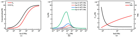
Figure 13.
The relationship between the association rate constant ka and LFIA detection performance. (a) Variation in ST and SC under different association rate constants ka; (b) standard curves of the HOOK effect under different association rate constants ka; (c) trends in LFIA detection limits and working ranges under different association rate constants ka.
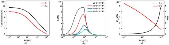
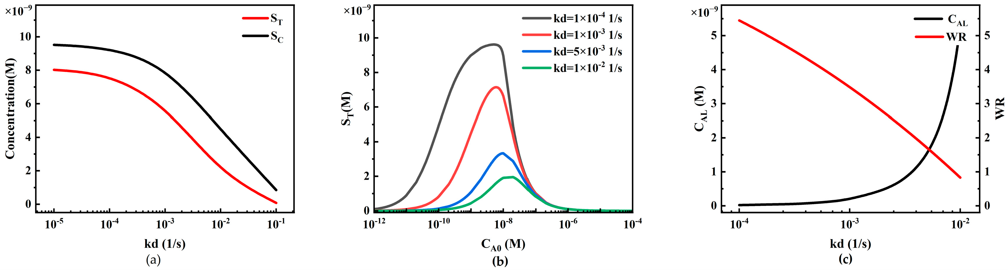
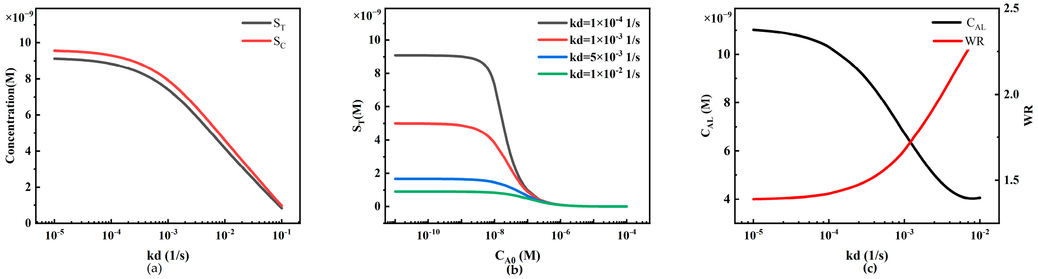
Figure 14.
The relationship between the dissociation rate constant kd and LFIA detection performance. (a) Variations in ST and SC under different dissociation rate constants kd; (b) standard curves of the HOOK effect under different dissociation rate constants kd; (c) trends in LFIA detection limits and working ranges under different dissociation rate constants kd.
From Figure 13a, we observe the variations in ST and SC under different association rate constants ka at constant analyte concentrations. A larger ka implies improved reaction efficiency of the reagents, resulting in higher ST and SC at the T-line and C-line. However, when the binding sites of the capture probes on the T-line and C-line become saturated, ST and SC tend to saturate as well.
In Figure 13b, we observe the phenomenon of the HOOK effect under different association rate constants (ka = 1 × 10⁵, 5 × 10⁵, 1 × 10⁶, 1 × 10⁷ M−1 s−1). An increase in ka significantly shifts the peak of the HOOK curve to the left (lower analyte concentrations). From Figure 13b, we extract the system detection limit (CAL) and working range (WR) (Figure 13c). With an increase in ka, the detection limit decreases significantly, and the working range gradually expands. This is mainly because higher ka enhances the reaction efficiency of the reagents, leading to greater capture efficiency of the capture probes on the test line and stronger binding capacity.
The impact of the dissociation rate constant kd on system performance is exactly the opposite of the association rate constant ka (Figure 14). An increase in kd leads to a decrease in the reaction rate, significantly reducing the capture capacity of the T-line and C-line, resulting in a decrease in ST and SC (Figure 14a). In the HOOK effect curves at different analyte concentrations (Figure 14b), an increase in kd leads to a rightward shift in the curve peak, indicating an increase in the detection limit, which reduces the sensitivity of the system, while the working range also narrows (Figure 14c).
These phenomena indicate that increasing the association rate ka and decreasing the dissociation rate kd are beneficial for quantitative analysis in rapid LFIA detection. By selecting antibodies or capture probes with higher association rate constants and lower dissociation rate constants, we can optimize the performance of LFIA detection. However, it is important to note that antibodies or capture probes with higher association rates may be accompanied by higher dissociation rates. Therefore, when designing LFIA, a balanced consideration between association and dissociation rates is needed to achieve optimal performance.
4.3. Competitive LFIA
4.3.1. Competitive LFIA Reaction Process
Similarly to the sandwich LFIA, we explored the reaction process of competitive LFIA under non-uniform fluid flow conditions (Figure 15). The concentration distribution of analytes A, reporter particles P, and analyte–reporter particle complexes PA in competitive LFIA is similar to that in sandwich LFIA, and will not be repeated here. The concentration distribution of complexes RTP captured by the T-line, PA captured by the C-line, and complexes RCPA and RCP formed by PA and P capture is shown in Figure 15a. Under the same conditions, the color of the T-line in competitive LFIA is darker. This is because in sandwich LFIA, part of the T-line capture probe reacts with A in the analyte, resulting in a reduction in binding sites and a decrease in the capture capability for free reporter particles P.

Figure 15.
Competitive LFIA reaction process. (a) Concentration distribution map of reporter particle complexes captured by T-line and C-line; (b) variation in T-line and C-line signals ST and SC over time; (c) diffusion effects of reporter particle complexes captured by T-line and C-line.
Figure 15b depicts the variation in T-line and C-line signals ST and SC over time. According to the reaction kinetics equation, the T-line only captures free reporter particles P, while the C-line captures not only free reporter particles P but also the reporter particle–analyte complex PA. Therefore, after the reaction reaches equilibrium, SC is higher than ST.
Figure 15c describes the distribution of product concentration along the x-direction on the surfaces of the T-line and C-line. Similarly to sandwich LFIA, competitive LFIA exhibits edge effects in the concentration distribution along the surfaces of the T-line and C-line, with stronger signals at the edges of the T-line and C-line.
4.3.2. The Influence of Target Analyte Concentration on ST and SC in Competitive LFIA
The influence of target analyte concentration on ST follows a sigmoidal curve (Figure 16), which is a typical form of calibration curves in competitive analysis [30]. When the target analyte concentration is low, the analytes A have little effect on the concentration of free reporter particles P, resulting in a high and relatively constant ST value. As the analyte concentration increases, the competitive reaction between analytes A and reporter particles P intensifies, leading to a decrease in the concentration of free reporter particles P and a nearly linear decrease in ST. When the analyte concentration reaches a certain level, the competitive reaction between analytes A and reporter particles P saturates, and ST no longer changes with increasing analyte concentration. SC, on the other hand, remains unaffected by changes in analyte concentration, which is why the T/C ratio is commonly used as the detection result in commercial assays.
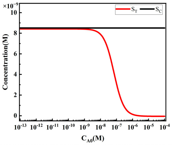
Figure 16.
Impact of target analyte concentration on ST and SC.
4.3.3. The Influence of Reporter Particle Concentration on Competitive LFIA Performance
Similarly to the sandwich LFIA, we first analyze the effect of reporter particle concentration on the performance of competitive LFIA (Figure 17). Under constant analyte concentration conditions, the trends of ST and SC at different reporter particle concentrations are similar to those in the sandwich LFIA. At low CP0 concentrations, the changes in ST and SC are minimal. As CP0 increases, both ST and SC linearly depend on CP0. Followed by a slower growth rate, this is due to the saturation of binding sites for capture probes on the T-line and C-line.
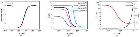
Figure 17.
The relationship between reporter particle concentration and LFIA detection performance. (a) Variations in ST and SC under different reporter particle concentrations. (b) Inverse S-shaped standard curves at different reporter particle concentrations. (c) Trends of LFIA detection limits and working ranges under different reporter particle concentrations.
We also plotted inverse S-shaped standard curves for different CP0 values (1 × 10⁻⁹, 5 × 10⁻⁹, 1 × 10⁻⁸, and 1 × 10⁻⁷ M) (Figure 17b). The increase in CP0 results in a rightward shift in the curve, with both detection limit and working range moving towards higher analyte concentrations. This is because as CP0 increases, more reporter particles can bind to more target analytes to form reporter particle–analyte complexes PA. However, due to competitive effects, this hinders the recognition and capture of reporter particles by the T-line capture probes.
To further compare LFIA performance, we extracted detection limits (CAL) and working ranges (WR) from simulation results (Figure 17c). As CP0 increases, CAL shows an upward trend in the simulation (black line in Figure 17c), indicating that higher CP0 actually decreases system sensitivity, with this effect becoming more pronounced at higher concentrations. Additionally, it can be observed from the simulation results that as CP0 increases, WR narrows (red line in Figure 17c). Unlike the sandwich LFIA, an increase in CP0 actually raises the system detection limit and narrows the working range, consistent with the conclusion in reference [30]. This suggests that higher CP0 concentrations increase the detection signal strength, but reducing CP0 can be used to enhance the detection sensitivity of competitive LFIA. We can utilize this model to predict standard curves, CAL, and WR under different CP0 values and assist experimenters in selecting the optimal CP0 for LFIA performance.
4.3.4. The Influence of Capture Probe Initial Concentration on Competitive LFIA Performance
Similarly to the sandwich LFIA, the initial concentration of the T-line capture probe, CRT0, only affects ST and has minimal impact on SC (Figure 18a). When CRT0 is low, it fails to effectively capture reporter particles and analytes, resulting in lower and relatively unchanged ST. As the concentration of capture antibodies increases, the capturing capability enhances, leading to an almost linear increase in ST. However, at high CRT0 concentrations, ST decreases instead. This might be attributed to the limited binding capacity of proteins on the membrane, causing protein accumulation and spatial hindrance effects when CRT0 concentration is too high, inhibiting the capture reaction of reporter particles P. As ST almost linearly increases, more reporter particles P are captured by the T-line, reducing the concentration of reporter particles CP0 downstream of the T-line and thus lowering SC.
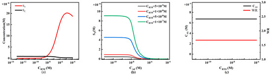
Figure 18.
The Relationship between T-Line Capture Probe Initial Concentration and LFIA Detection Performance: (a) Variations in ST and SC under Different T-Line Capture Probe Initial Concentrations; (b) Inverse S-shaped Standard Curves under Different T-Line Capture Probe Initial Concentrations; (c) Trends of LFIA Detection Limits and WR under Different T-Line Capture Probe Initial Concentrations.
We plotted inverse S-shaped curves for ST at different analyte concentrations using different CRT0 values (5 × 10⁻⁹, 1 × 10⁻⁸, 5 × 10⁻⁸, and 1 × 10⁻⁷ M) (Figure 18b). The increase in CRT0 enhances the capturing capability of the T-line, resulting in a higher maximum value of the ST curve, which generates a stronger signal. However, changes in CRT0 have no significant impact on the detection limits and working ranges calculated using the metrics in this study (Figure 18c).
The effect of C-line capture probe initial concentration, CRC0, on competitive LFIA performance is similar to that in the sandwich LFIA and will not be further elaborated here.
4.3.5. The Influence of Reaction Constants on Competitive LFIA Performance
The effects of reaction constants ka and kd on competitive LFIA performance are depicted in Figure 19 and Figure 20. From Figure 19a and Figure 20a, we observe the variations in ST and SC at different values of ka and kd while holding the analyte concentration constant. Larger values of ka and lower values of kd enhance the efficiency of the reaction, resulting in higher ST and SC on both the T-line and C-line, which gradually saturate.
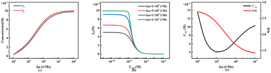
Figure 19.
The relationship between association rate constant ka and LFIA detection performance: (a) Variations in ST and SC under different association rate constants ka; (b) inverse S-shaped standard curves under different association rate constants ka; (c) trends of LFIA detection limits and working ranges under different association rate constants ka.
Figure 20.
The relationship between dissociation rate constant kd and LFIA detection performance: (a) variations in ST and SC under different dissociation rate constants kd; (b) inverse S-shaped standard curves under different dissociation rate constants kd; (c) trends of LFIA detection limits and working ranges under different dissociation rate constants kd.
Figure 19b and Figure 20b depict the inverse S-curves under different binding rate constants (ka = 1 × 10⁵, 5 × 10⁵, 1 × 10⁶, 1 × 10⁷ M−1 s−1) and different dissociation constants (kd = 1 × 10⁻⁴, 1 × 10⁻³, 5 × 10⁻³, 1 × 10⁻² s−1). Increasing ka and decreasing kd significantly narrow the working range (WR) (Figure 19c and Figure 20c). It also increases the system’s detection limit, which is detrimental to detection. These observations indicate that contrary to sandwich LFIA, increasing the binding rate ka and decreasing the dissociation rate kd can enhance the intensity of detection signals on both the T-line and C-line, but they have negative implications for the system’s detection limit and working range.
5. Conclusions
This paper uses the Richards equation to solve the capillary flow velocity model and couples the solved velocity field with the physical field of mass transfer in porous media to establish a three-dimensional LFIA model, investigating the reaction mechanism of LFIA under non-uniform flow conditions. The influence of pore size and porosity on flow velocity is explored, and the performance of LFIA under different average flow velocities is compared. Additionally, the transport and diffusion of various reaction components in sandwich LFIA and competitive LFIA are studied. Furthermore, the effects of analyte concentration, report particle concentration, capture probe concentration, and reaction constants on LFIA performance are analyzed. The conclusions are as follows:
- (1)
- The sample flow velocity decreases exponentially with the distance from the sample front to the origin. Increasing the pore size and porosity of the membrane both increase the capillary flow velocity, thus reducing the sensitivity of LFIA.
- (2)
- In sandwich LFIA, appropriately increasing the report particle concentration CP0, increasing the initial concentration of T-line capture probe CRT0, increasing the binding rate ka, and decreasing the dissociation rate kd are all beneficial for reducing the detection limit and broadening the working range of LFIA. The initial concentration of C-line capture probe CRC0 has little effect on LFIA performance but lowers the T/C ratio.
- (3)
- For competitive LFIA, increasing the report particle concentration CP0, increasing the binding rate ka, and decreasing the dissociation rate kd may adversely affect the detection limit and working range of LFIA. Under the indicators of this paper, the effect of T-line CRT0 on LFIA performance is insensitive.
The three-dimensional simulation model proposed in this paper has multiple applications in LFIA. Firstly, it allows for a comprehensive understanding of LFIA’s flow characteristics and reaction mechanisms, thereby enabling the prediction of LFIA’s detection limit and working range, ultimately enhancing detection sensitivity and accuracy. Secondly, the model can guide the design and optimization of LFIA products, including optimizing fluid channel design and reagent injection methods to improve equipment performance and stability. Additionally, the model can be used to validate the effectiveness and feasibility of new LFIA technologies or improvement methods, facilitating the application and promotion of new technologies. Lastly, the model can provide recommendations for product improvement and optimization, such as adjusting reagent formulations and optimizing operational procedures to enhance product performance and competitiveness. In summary, the LFIA three-dimensional simulation model serves as a valuable tool and support for the research, development, and application of LFIA technology, with the potential to play a significant role in medical diagnosis, food safety, environmental monitoring, and other fields.
Author Contributions
Conceptualization, X.Z. and L.W.; methodology, X.Z.; software, X.Z. and C.X.; validation, C.X. and Q.W.; formal analysis, H.B.; investigation, X.Z. and Q.N.; resources, Y.Z.; data curation, X.Z. and C.X.; writing—original draft preparation, X.Z.; writing—review and editing, L.W.; visualization, X.Z. and C.X.; supervision, Y.Z. and Q.N.; project administration, Y.Z., L.W. and Q.N.; All authors have read and agreed to the published version of the manuscript.
Funding
This work was supported by the Innovative Funds Plan of Henan University of Technology (No. 2022ZKCJ03) and Henan Science and Technology Research Program (No. 201300210100).
Data Availability Statement
The data that support the findings of this study are available within the article.
Acknowledgments
We would like to express our sincere gratitude to all those who contributed to this research project. Special thanks to Henan University of Technology for their financial support.
Conflicts of Interest
The authors declare no conflicts of interest.
References
- Di Nardo, F.; Chiarello, M.; Cavalera, S.; Baggiani, C.; Anfossi, L. Ten Years of Lateral Flow Immunoassay Technique Applications: Trends, Challenges and Future Perspectives. Sensors 2021, 21, 33. [Google Scholar] [CrossRef] [PubMed]
- Wu, P.C.; Song, J.R.; Sun, C.X.; Zuo, W.C.; Dai, J.J.; Ju, Y.M. Recent advances of lateral flow immunoassay for bacterial detection: Capture-antibody-independent strategies and high-sensitivity detection technologies. TrAC Trends Anal. Chem. 2023, 166, 16. [Google Scholar]
- Barshevskaya, L.V.; Sotnikov, D.V.; Zherdev, A.V.; Khassenov, B.B.; Baltin, K.K.; Eskendirova, S.Z.; Mukanov, K.K.; Mukantayev, K.K.; Dzantiev, B.B. Triple Immunochromatographic System for Simultaneous Serodiagnosis of Bovine Brucellosis, Tuberculosis, and Leukemia. Biosensors 2019, 9, 10. [Google Scholar] [CrossRef] [PubMed]
- Liu, H.F.; Dai, E.H.; Xiao, R.; Zhou, Z.H.; Zhang, M.L.; Bai, Z.K.; Shao, Y.; Qi, K.Z.; Tu, J.; Wang, C.W.; et al. Development of a SERS-based lateral flow immunoassay for rapid and ultra-sensitive detection of anti-SARS-CoV-2 IgM/IgG in clinical samples. Sens. Actuator B Chem. 2021, 329, 10. [Google Scholar] [CrossRef]
- Sotnikov, D.V.; Barshevskaya, L.V.; Bartosh, A.V.; Zherdev, A.V.; Dzantiev, B.B. Double Competitive Immunodetection of Small Analyte: Realization for Highly Sensitive Lateral Flow Immunoassay of Chloramphenicol. Biosensors 2022, 12, 10. [Google Scholar] [CrossRef] [PubMed]
- Li, W.B.; Wang, Z.D.; Wang, X.W.; Cui, L.; Huang, W.Y.; Zhu, Z.Y.; Liu, Z.J. Highly efficient detection of deoxynivalenol and zearalenone in the aqueous environment based on nanoenzyme-mediated lateral flow immunoassay combined with smartphone. J. Environ. Chem. Eng. 2023, 11, 9. [Google Scholar] [CrossRef]
- Willemsen, L.; Wichers, J.; Xu, M.; Van Hoof, R.; Van Dooremalen, C.; Van Amerongen, A.; Peters, J. Biosensing Chlorpyrifos in Environmental Water Samples by a Newly Developed Carbon Nanoparticle-Based Indirect Lateral Flow Assay. Biosensors 2022, 12, 13. [Google Scholar] [CrossRef]
- Hua, Q.C.; Liu, Z.W.; Wang, J.; Liang, Z.Q.; Zhou, Z.X.; Shen, X.; Lei, H.T.; Li, X.M. Magnetic immunochromatographic assay with smartphone-based readout device for the on-site detection of zearalenone in cereals. Food Control 2022, 134, 11. [Google Scholar] [CrossRef]
- Wild, D. (Ed.) The Immunoassay Handbook: Theory and Applications of Ligand Binding, ELISA and Related Techniques; People’s Medical Publishing House: Beijing, China, 2021; pp. 6–8. [Google Scholar]
- Datta, P. Immunoassay design. In Accurate Results in the Clinical Laboratory; Elsevier: Amsterdam, The Netherlands, 2019; pp. 69–73. [Google Scholar]
- Zhang, G. Rapid Detection Technology of Immunochromatographic Test Strips; Henan Science and Technology Press: Zhengzhou, China, 2015; pp. 8–11. [Google Scholar]
- Tong, L.; Li, D.Q.; Huang, M.; Huang, L.; Wang, J. Gold-Silver Alloy Nanoparticle-Incorporated Pitaya-Type Silica Nanohybrids for Sensitive Competitive Lateral Flow Immunoassay. Anal. Chem. 2023, 95, 17318–17327. [Google Scholar] [CrossRef]
- Jia, J.H.; Ao, L.J.; Luo, Y.X.; Liao, T.; Huang, L.; Zhuo, D.; Jiang, C.X.; Wang, J.; Hu, J. Quantum dots assembly enhanced and dual-antigen sandwich structured lateral flow immunoassay of SARS-CoV-2 antibody with simultaneously high sensitivity and specificity. Biosens. Bioelectron. 2022, 198, 8. [Google Scholar] [CrossRef]
- Wang, X.; Yang, D.; Jia, S.T.; Zhao, L.L.; Jia, T.T.; Xue, C.H. Electrospun nitrocellulose membrane for immunochromatographic test strip with high sensitivity. Microchim. Acta 2020, 187, 644. [Google Scholar] [CrossRef]
- Lin, D.; Li, B.; Fu, L.; Qi, J.; Xia, C.; Zhang, Y.; Chen, L. A novel polymer-based nitrocellulose platform for implementing a multiplexed microfluidic paper-based enzyme-linked immunosorbent assay. Microsyst. Nanoeng. 2022, 8, 53. [Google Scholar] [CrossRef]
- Christopoulou, N.M.; Kalogianni, D.P.; Christopoulos, T.K. Macromolecular crowding agents enhance the sensitivity of lateral flow immunoassays. Biosens. Bioelectron. 2022, 218, 8. [Google Scholar] [CrossRef]
- Liu, X.J.; Chen, Y.Q.; Bu, T.; Deng, Z.I.; Zhao, L.; Tian, Y.L.; Jia, C.H.; Li, Y.C.; Wang, R.; Wang, J.L.; et al. Nanosheet antibody mimics based label-free and dual-readout lateral flow immunoassay for Salmonella enteritidis rapid detection. Biosens. Bioelectron. 2023, 229, 7. [Google Scholar] [CrossRef]
- Zadehkafi, A.; Siavashi, M.; Asiaei, S.; Bidgoli, M.R. Simple geometrical modifications for substantial color intensity and detection limit enhancements in lateral-flow immunochromatographic assays. J. Chromatogr. B 2019, 1110, 1–8. [Google Scholar] [CrossRef]
- Díaz-González, M.; de la Escosura-Muñiz, A. Strip modification and alternative architectures for signal amplification in nanoparticle-based lateral flow assays. Anal. Bioanal. Chem. 2021, 413, 4111–4117. [Google Scholar] [CrossRef]
- Schaumburg, F.; Kler, P.A.; Berli, C.L.A. Numerical prototyping of lateral flow biosensors. Sens. Actuator B Chem. 2018, 259, 1099–1107. [Google Scholar] [CrossRef]
- Jeon, M.J.; Kim, S.-K.; Hwang, S.-H.; Lee, J.U.; Sim, S.J. Lateral flow immunoassay based on surface-enhanced Raman scattering using pH-induced phage-templated hierarchical plasmonic assembly for point-of-care diagnosis of infectious disease. Biosens. Bioelectron. 2024, 250, 116061. [Google Scholar] [CrossRef] [PubMed]
- Kunpatee, K.; Khantasup, K.; Komolpis, K.; Yakoh, A.; Nuanualsuwan, S.; Sain, M.M.; Chaiyo, S. Ratiometric electrochemical lateral flow immunoassay for the detection of Streptococcus suis serotype 2. Biosens. Bioelectron. 2023, 242, 7. [Google Scholar] [CrossRef] [PubMed]
- Zhang, G.; Hu, H.; Deng, S.L.; Xiao, X.Y.; Xiong, Y.H.; Peng, J.; Lai, W.H. An integrated colorimetric and photothermal lateral flow immunoassay based on bimetallic Ag-Au urchin-like hollow structures for the sensitive detection of E. coli O157:H7. Biosens. Bioelectron. 2023, 225, 10. [Google Scholar] [CrossRef] [PubMed]
- Roy, L.; Buragohain, P.; Borse, V. Strategies for sensitivity enhancement of point-of-care devices. Biosens. Bioelectron. 2022, 10, 100098. [Google Scholar] [CrossRef]
- Gasperino, D.; Baughman, T.; Hsieh, H.V.; Bell, D.; Weigl, B.H. Improving Lateral Flow Assay Performance Using Computational Modeling. In Annual Review of Analytical Chemistry; Bohn, P.W., Pemberton, J.E., Eds.; Annual Reviews: Palo Alto, CA, USA, 2018; Volume 11, pp. 219–244. [Google Scholar]
- Qian, S.; Bau, H.H. A mathematical model of lateral flow bioreactions applied to sandwich assays. Anal. Biochem. 2003, 322, 89–98. [Google Scholar] [CrossRef]
- Qian, S.; Bau, H.H. Analysis of lateral flow biodetectors: Competitive format. Anal. Biochem. 2004, 326, 211–224. [Google Scholar] [CrossRef]
- Berli, C.L.A.; Kler, P.A. A quantitative model for lateral flow assays. Microfluid. Nanofluid. 2016, 20, 9. [Google Scholar] [CrossRef]
- Sotnikov, D.V.; Zherdev, A.V.; Dzantiev, B.B. Mathematical Model of Serodiagnostic Immunochromatographic Assay. Anal. Chem. 2017, 89, 4419–4427. [Google Scholar] [CrossRef] [PubMed]
- Sotnikov, D.V.; Byzova, N.A.; Zvereva, E.A.; Bartosh, A.V.; Zherdev, A.V.; Dzantiev, B.B. Mathematical modeling of immunochromatographic test systems in a competitive format: Analytical and numerical approaches. Biochem. Eng. J. 2020, 164, 9. [Google Scholar] [CrossRef]
- Liu, Z.; Hu, J.; Li, A.; Feng, S.S.; Qu, Z.G.; Xu, F. The effect of report particle properties on lateral flow assays: A mathematical model. Sens. Actuator B Chem. 2017, 248, 699–707. [Google Scholar] [CrossRef]
- Liu, Z.; Qu, Z.G.; Tang, R.H.; He, X.C.; Yang, H.; Bai, D.; Xu, F. An improved detection limit and working range of lateral flow assays based on a mathematical model. Analyst 2018, 143, 2775–2783. [Google Scholar] [CrossRef]
- Liu, Z.; He, X.C.; Li, A.; Qu, Z.G.; Xu, F. A two-dimensional mathematical model for analyzing the effects of capture probe properties on the performance of lateral flow assays. Analyst 2019, 144, 5394–5403. [Google Scholar] [CrossRef]
- Asadi, H.; Pourjafar-Chelikdani, M.; Khabazi, N.P.; Sadeghy, K. Quasi-steady imbibition of physiological liquids in paper-based microfluidic kits: Effect of shear-thinning. Phys. Fluids 2022, 34, 15. [Google Scholar] [CrossRef]
- Simulating Rapid Detection in COMSOL Multiphysics®. Available online: http://cn.comsol.com/blogs/modeling-a-rapid-detection-test-in-comsol-multiphysics/ (accessed on 16 August 2023).
- Tay, D.M.; Kim, S.; Hao, Y.; Yee, E.H.; Jia, H.; Vleck, S.M.; Sikes, H.D. Accelerating the optimization of vertical flow assay performance guided by a rational systematic model-based approach. Biosens. Bioelectron. 2023, 222, 114977. [Google Scholar] [CrossRef] [PubMed]
- Mendez, S.; Fenton, E.M.; Gallegos, G.R.; Petsev, D.N.; Sibbett, S.S.; Stone, H.A. Imbibition in porous membranes of complex shape: Quasi-stationary flow in thin rectangular segments. Langmuir 2010, 26, 1380–1385. [Google Scholar] [CrossRef] [PubMed]


Disclaimer/Publisher’s Note: The statements, opinions and data contained in all publications are solely those of the individual author(s) and contributor(s) and not of MDPI and/or the editor(s). MDPI and/or the editor(s) disclaim responsibility for any injury to people or property resulting from any ideas, methods, instructions or products referred to in the content. |
© 2024 by the authors. Licensee MDPI, Basel, Switzerland. This article is an open access article distributed under the terms and conditions of the Creative Commons Attribution (CC BY) license (https://creativecommons.org/licenses/by/4.0/).