


A Novel Experimental Apparatus for Characterizing Flow Regime in Mechanically Stirred Tanks through Force Sensors


Abstract
:
1. Introduction
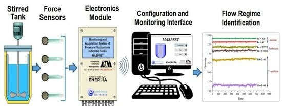
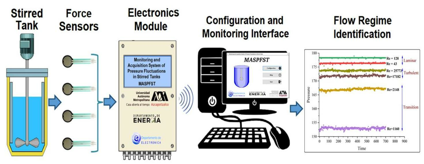
2. Design of the Apparatus
2.1. Sensor Features
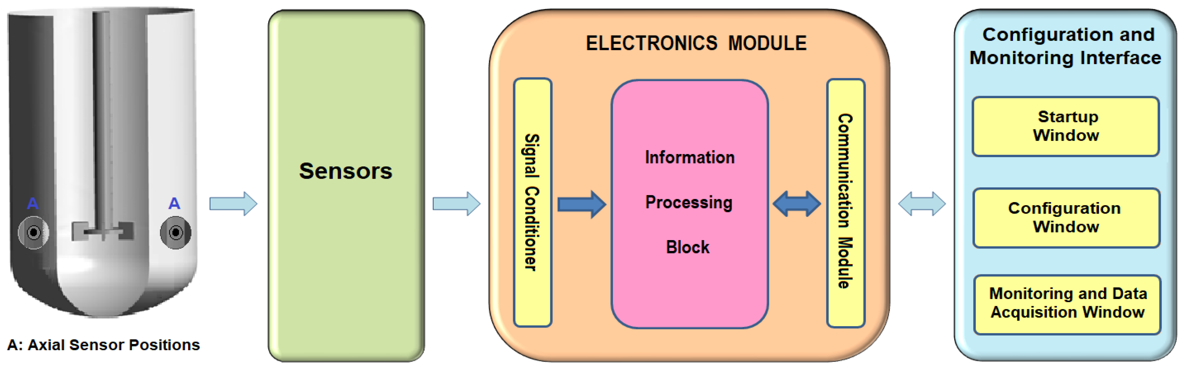
2.2. Electronics Module
2.2.1. Signal Conditioning
2.2.2. Communication Module
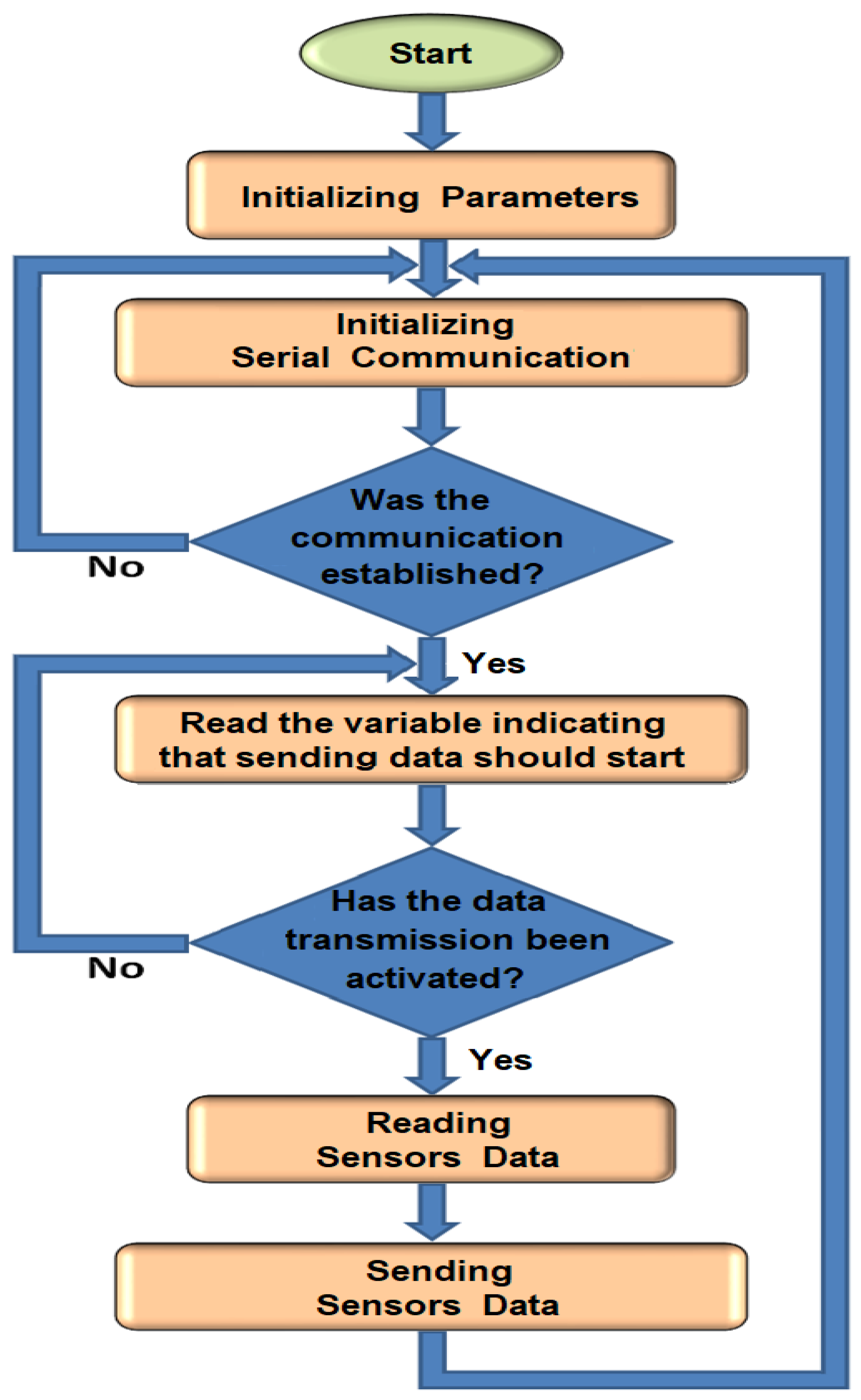
2.2.3. Information Processing Block
2.3. Configuration and Monitoring Interface
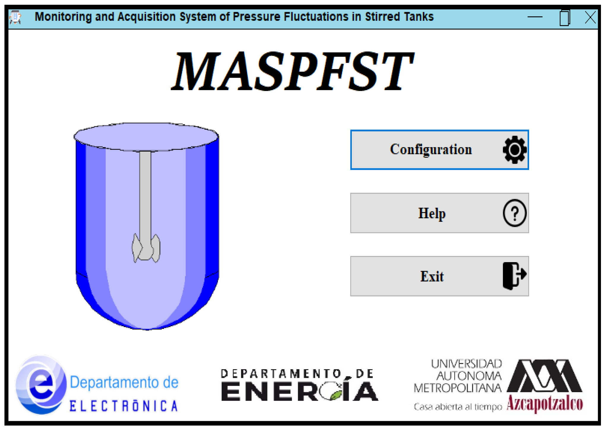
2.3.1. Startup Window
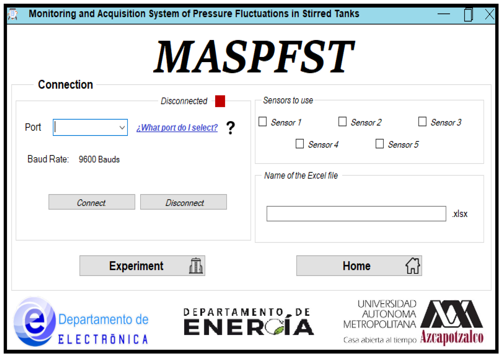
2.3.2. Configuration Window
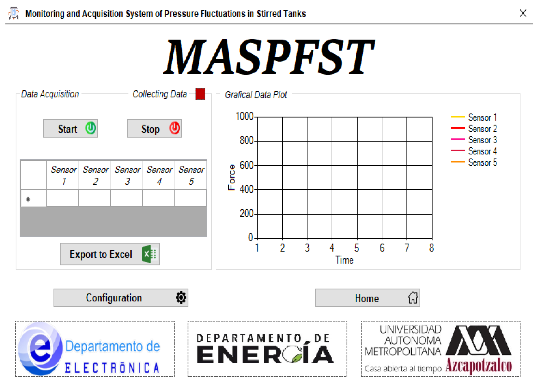
2.3.3. Monitoring and Data Acquisition Window
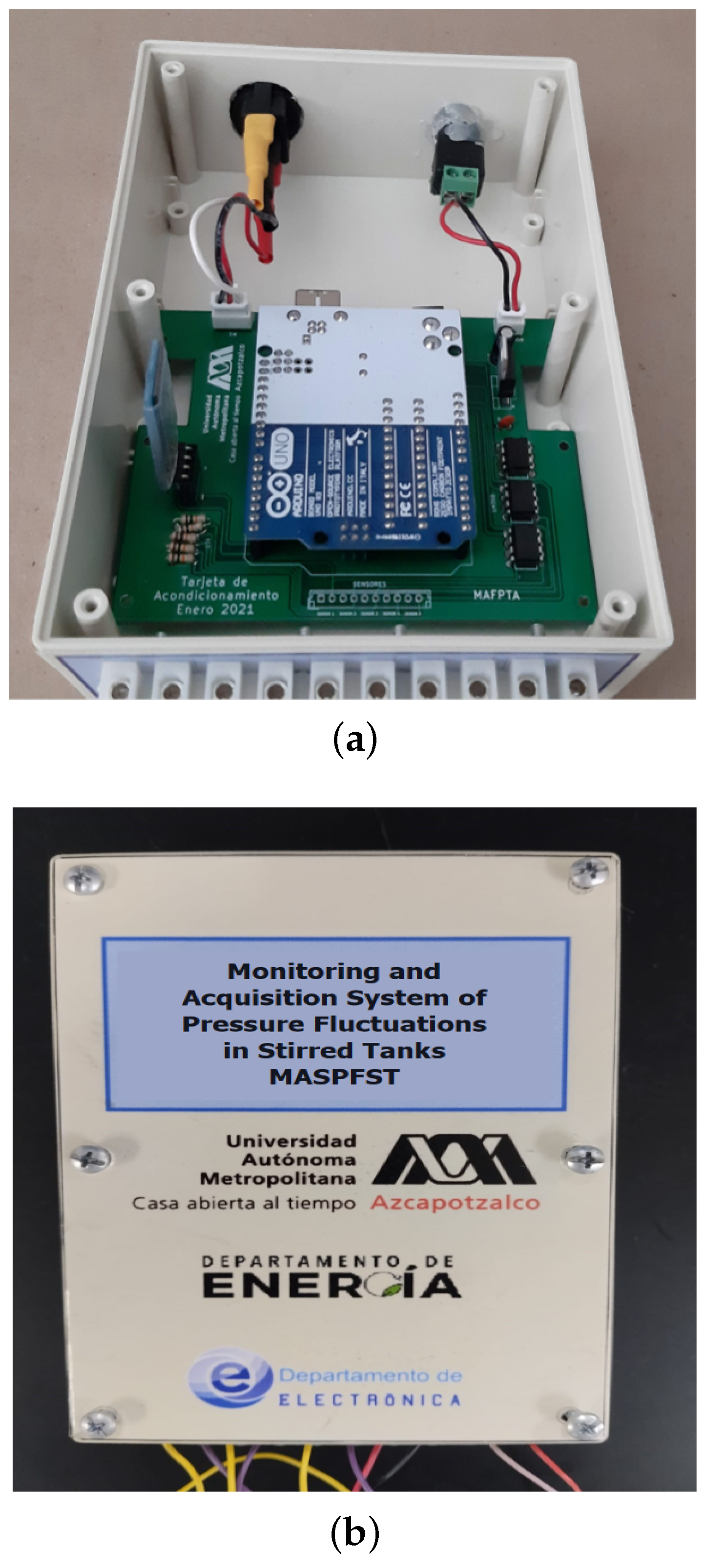
3. Apparatus Construction
4. Performance Tests
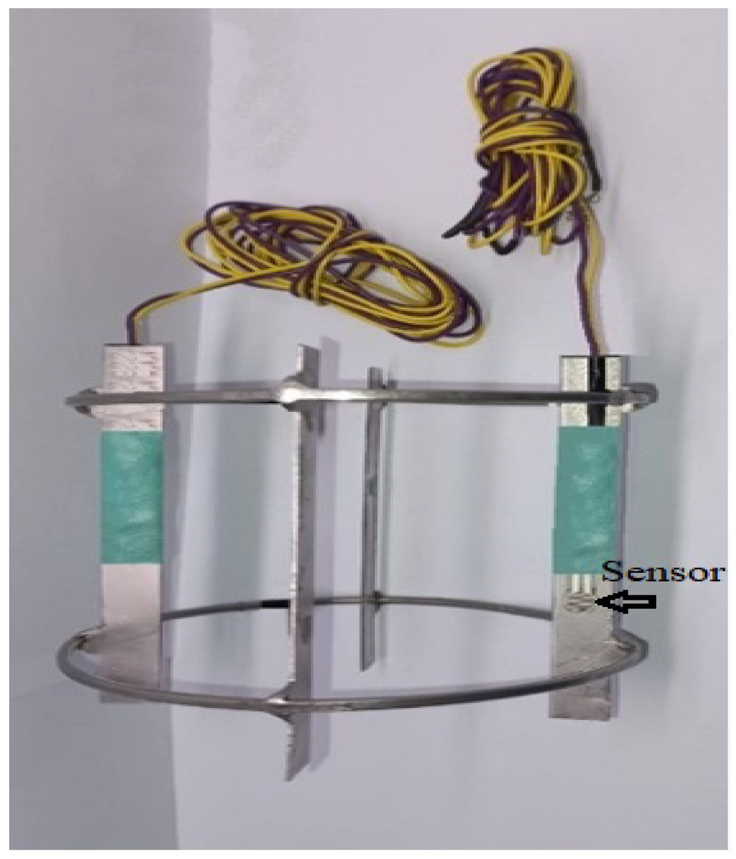
4.1. Baffle and Sensors
4.2. Monitoring and Acquisition System
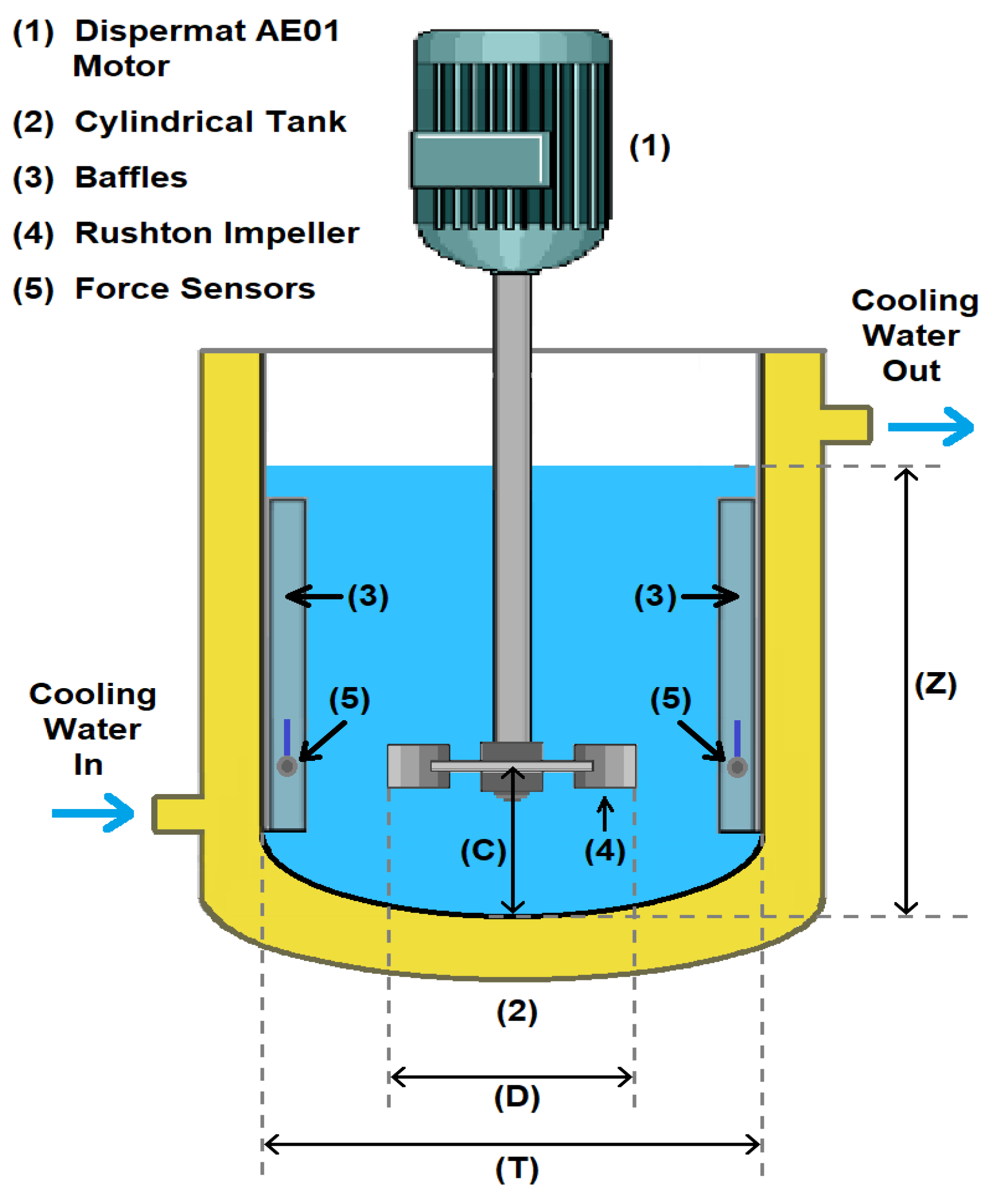
4.3. Agitation System and Mixing Tank Experiments
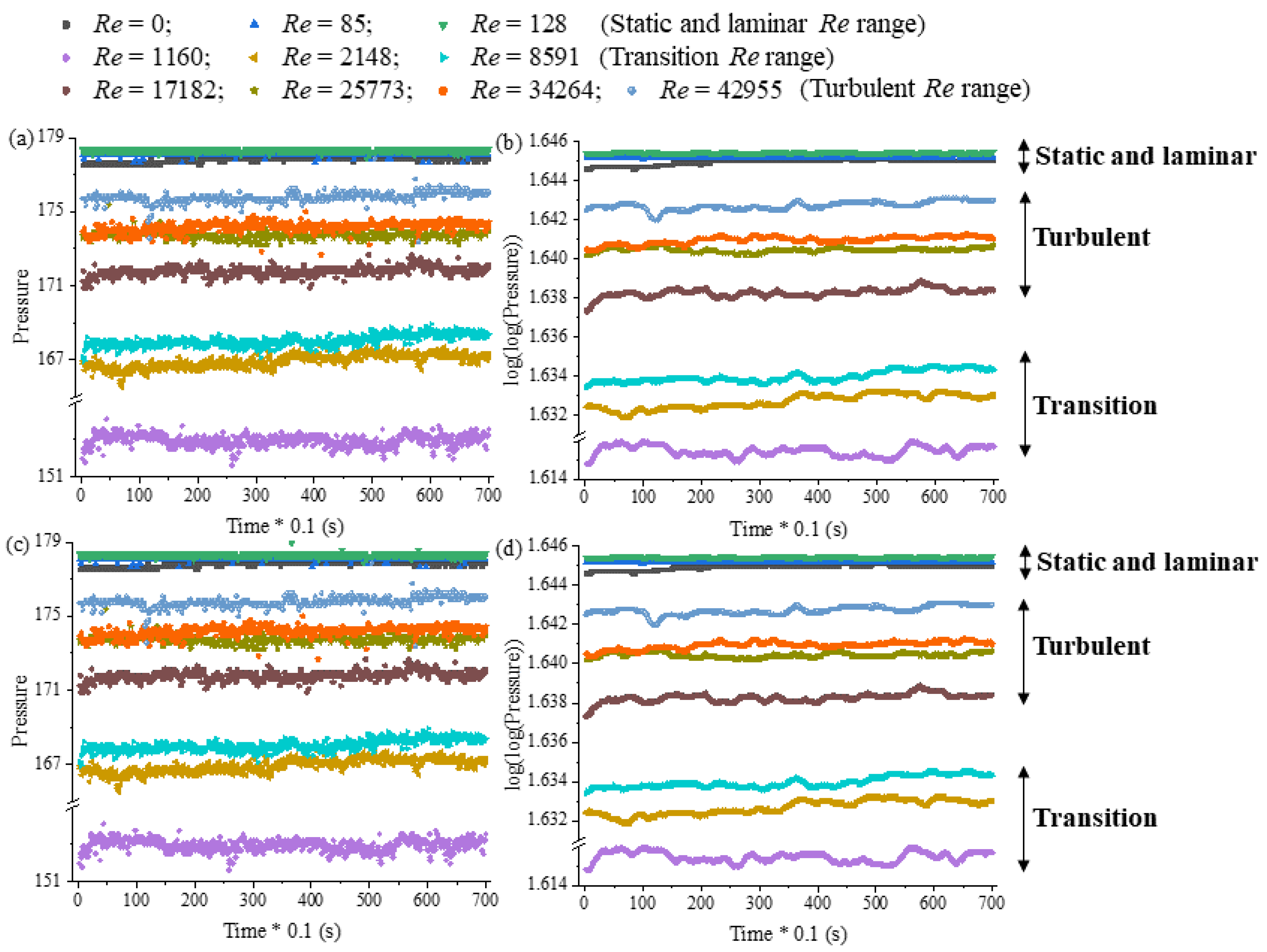
4.4. Analysis of Pressure Fluctuations
5. Conclusions
Author Contributions
Funding
Institutional Review Board Statement
Informed Consent Statement
Data Availability Statement
Conflicts of Interest
References
- Watson, N.J.; Bowler, A.L.; Rady, A.; Fisher, O.J.; Simeone, A.; Escrig, J.; Woolley, E.; Adedeji, A.A. Intelligent Sensors for Sustainable Food and Drink Manufacturing. Front. Sustain. Food Syst. 2021, 5, 642786. [Google Scholar] [CrossRef]
- Tang, X.; Pionteck, J.; Pötschke, P. Improved piezoresistive sensing behavior of poly(vinylidene fluoride)/carbon black composites by blending with a second polymer. Polymer 2023, 268, 125702. [Google Scholar] [CrossRef]
- Osho, S.; Wu, N.; Aramfard, M.; Deng, C.; Ojo, O. Fabrication and calibration of a piezoelectric nanocomposite paint. Smart Mater. Struct. 2018, 27, 035007. [Google Scholar] [CrossRef]
- Li, R.; Fu, L.; Zhang, J.; Wang, W.; Chen, X.; Zhao, J.; Han, D. Solid-liquid equilibrium and thermodynamic properties of dipyridamole form II in pure solvents and mixture of (N-methyl pyrrolidone + isopropanol). J. Chem. Thermodyn. 2020, 142, 105981. [Google Scholar] [CrossRef]
- Mahar, R.; Chakraborty, A.; Nainwal, N. The influence of carrier type, physical characteristics, and blending techniques on the performance of dry powder inhalers. J. Drug Deliv. Sci. Technol. 2022, 76, 103759. [Google Scholar] [CrossRef]
- Bowler, A.L.; Bakalis, S.; Watson, N.J. A review of in-line and on-line measurement techniques to monitor industrial mixing processes. Chem. Eng. Res. Des. 2020, 153, 463–495. [Google Scholar] [CrossRef]
- Afshar Ghotli, R.; Abdul Raman, A.A.; Ibrahim, S. The effect of various designs of six-curved blade impellers on reaction rate analysis in liquid–liquid mixing vessel. Measurement 2016, 91, 440–450. [Google Scholar] [CrossRef]
- Ammar, M.; Driss, Z.; Chtourou, W.; Abid, M.S. Effect of the tank design on the flow pattern generated with a pitched blade turbine. Int. J. Mech. Appl. 2012, 2, 12–19. [Google Scholar] [CrossRef]
- Jiang, M.; Zhao, Y.; Liu, G.; Zheng, J. Enhancing mixing of particles by baffles in a rotating drum mixer. Particuology 2011, 9, 270–278. [Google Scholar] [CrossRef]
- Hockmeyer, H. Practical guide to high-speed dispersion. Paint. Coat. Ind. 2010, 26, 32–36. [Google Scholar]
- Ramírez-Muñoz, J.; Márquez-Baños, V.; Alvarez-Vega, J.; Mompremier, R.; Gómez Núñez, J.; Guadarrama-Pérez, R. Hydrodynamics performance of Newtonian and shear-thinning fluids in a tank stirred with a high shear impeller: Effect of liquid height and off-bottom clearance. Chem. Eng. Res. Des. 2023, 192, 44–54. [Google Scholar] [CrossRef]
- Fasano, J.B.; Bakker, A.; Penney, W.R. Advanced impeller geometry boosts liquid agitation. Chem. Eng. 1994, 101, 110. [Google Scholar]
- Paul, E.L.; Atlemo-Obeng, V.A.; Kresta, S.M. Handbook of Industrial Mixing: Science and Practice; John Wiley & Sons, Inc.: Hoboken, NJ, USA, 2004. [Google Scholar]
- Zhan, X.; Yang, Y.; Liang, J.; Shi, T.; Li, X. Gas Bubble Effects and Elimination in Ultrasonic Measurement of Particle Concentrations in Solid–Liquid Mixing Processes. IEEE Trans. Instrum. Meas. 2017, 66, 1711–1718. [Google Scholar] [CrossRef]
- Bamberger, J.A.; Greenwood, M.S. Using ultrasonic attenuation to monitor slurry mixing in real time. Ultrasonics 2004, 42, 145–148. [Google Scholar] [CrossRef] [PubMed]
- Fox, P.; Smith, P.P.; Sahi, S. Ultrasound measurements to monitor the specific gravity of food batters. J. Food Eng. 2004, 65, 317–324. [Google Scholar] [CrossRef]
- Slettengren, K.; Heunemann, P.; Knuchel, O.; Windhab, E.J. Mixing quality of powder-liquid mixtures studied by near infrared spectroscopy and colorimetry. Powder Technol. 2015, 278, 130–137. [Google Scholar] [CrossRef]
- Shenoy, P.; Innings, F.; Tammel, K.; Fitzpatrick, J.; Ahrné, L. Evaluation of a digital colour imaging system for assessing the mixture quality of spice powder mixes by comparison with a salt conductivity method. Powder Technol. 2015, 286, 48–54. [Google Scholar] [CrossRef]
- Mirshekari, F.; Pakzad, L. Mixing of Oil in Water Through Electrical Resistance Tomography and Response Surface Methodology. Chem. Eng. Technol. 2019, 42, 1101–1115. [Google Scholar] [CrossRef]
- Maluta, F.; Montante, G.; Paglianti, A. Analysis of immiscible liquid-liquid mixing in stirred tanks by Electrical Resistance Tomography. Chem. Eng. Sci. 2020, 227, 115898. [Google Scholar] [CrossRef]
- Yang, C.; Lu, H.; Wang, B.; Xu, Z.; Liu, B. Flow regime identification using pressure fluctuation signals in an aerated vessel stirred. Chem. Eng. Sci. 2023, 280, 119058. [Google Scholar] [CrossRef]
- Nienow, A.W. Effect of scale and geometry on flooding, recirculation and power in gassed stirred vessels. In Proceedings of the Second European Conference on Mixing, Cambridge, UK, 30 March–1 April 1977; pp. 1–16. [Google Scholar]
- Taghavi, M.; Zadghaffari, R.; Moghaddas, J.; Moghaddas, Y. Experimental and CFD investigation of power consumption in a dual Rushton turbine stirred tank. Chem. Eng. Res. Des. 2011, 89, 280–290. [Google Scholar] [CrossRef]
- Mosorov, V.; Rybak, G.; Sankowski, D. Plug regime flow velocity measurement problem based on correlability notion and twin plane electrical capacitance tomography: Use case. Sensors 2021, 21, 2189. [Google Scholar] [CrossRef] [PubMed]
- Ramakrishnan, V.; Arsalan, M. A Pressure-Based Multiphase Flowmeter: Proof of Concept. Sensors 2023, 23, 7267. [Google Scholar] [CrossRef] [PubMed]
- Ascanio, G.; Castro, B.; Galindo, E. Measurement of Power Consumption in Stirred Vessels—A Review. Chem. Eng. Res. Des. 2004, 82, 1282–1290. [Google Scholar] [CrossRef]
- Ramírez-Gomez, R.; García-Cortés, D.; Martínez-de Jesús, G.; González-Brambila, M.M.; Alonso, A.; Martínez-Delgadillo, S.A.; Ramírez-Muñoz, J. Performance Evaluation of Two High-Shear Impellers in an Unbaffled Stirred Tank. Chem. Eng. Technol. 2015, 38, 1519–1529. [Google Scholar] [CrossRef]
- Micaele, G.D.M.; Grisafi, F.; Brucato, A.; Ciofalo, M. Numerical Simulation of Low Reynolds Number Flow Fields in Unbaffled Stirred Vessels. In Proceedings of the 12th European Conference on Mixing, Bologna, Italy, 27–30 June 2006; pp. 57–64. [Google Scholar]
- Tamburini, A.; Gagliano, G.; Micale, G.; Brucato, A.; Scargiali, F.; Ciofalo, M. Direct numerical simulations of creeping to early turbulent flow in unbaffled and baffled stirred tanks. Chem. Eng. Sci. 2018, 192, 161–175. [Google Scholar] [CrossRef]
- De La Concha-Gómez, A.D.; Ramírez-Muñoz, J.; Márquez-Baños, V.E.; Haro, C.; Alonso-Gómez, A.R. Effect of the Rotating Reference Frame Size for Simulating a Mixing Straight-Blade Impeller an a Baffled Stirred Tank. Rev. Mex. Ing. Química 2019, 18, 1143–1160. [Google Scholar] [CrossRef]
- Bird, R.; Stewart, W.; Lightfoot, E. Transport Phenomena; John Wiley & Sons Inc.: New York, NY, USA, 2002. [Google Scholar]
- Pope, S.B. Turbulent Flows; Cambridge University Press: Cambridge, UK, 2000. [Google Scholar] [CrossRef]


| Signal | Terminal | Type |
|---|---|---|
| Voltage 5 V DC. | 5 V DC. | Output |
| Ground | GND | — |
| Ground | GND | — |
| Voltage 9 V DC | Vin | Input |
| Sensor 1 | A0 | Input |
| Sensor 2 | A1 | Input |
| Sensor 3 | A2 | Input |
| Sensor 4 | A3 | Input |
| Sensor 5 | A4 | Input |
| Serial port | TX | Output |
| Serial port | RX | Input |
| Ground | GND | — |
| Parameter | Usage |
|---|---|
| int sensorPin1 = A0; | Analog Input Sensor 1 |
| int sensorPin2 = A1; | Analog Input Sensor 2 |
| int sensorPin3 = A2; | Analog Input Sensor 3 |
| int sensorPin4 = A3; | Analog Input Sensor 4 |
| int sensorPin5 = A4; | Analog Input Sensor 5 |
| boolean KEY = false; | Flag for sending data |
| int mensaje = 0; | Data reading flag |
| void setup () {Serial.begin (9600);} | Communication at 9600 bps |
| Parameter | Value |
|---|---|
| Port | COM-8 |
| Baud Rate | 9600 |
| Sensor | 4 sensors |
| Name file | RowData.xls |
| Fluid | Density (kg · m−3) | Viscosity () | Reynolds Covered | Fluid Characteristics |
|---|---|---|---|---|
| 1 | 1110.80 | 0.0282 | Static and extended laminar flow | |
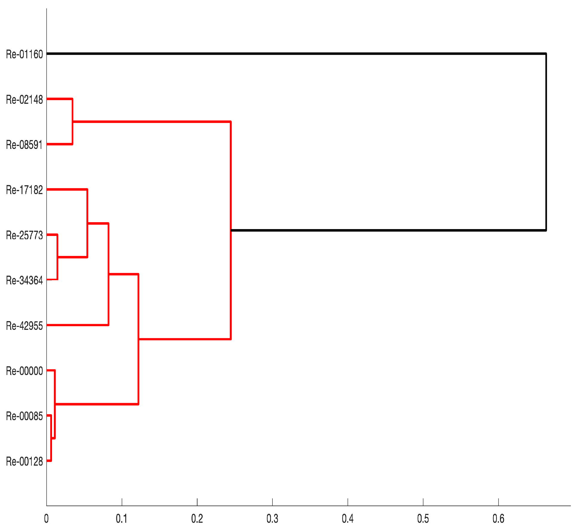
| 2 | 998.70 | 0.001 | 1160–42,955 | Turbulent transition to fully turbulent flow |
Disclaimer/Publisher’s Note: The statements, opinions and data contained in all publications are solely those of the individual author(s) and contributor(s) and not of MDPI and/or the editor(s). MDPI and/or the editor(s) disclaim responsibility for any injury to people or property resulting from any ideas, methods, instructions or products referred to in the content. |
© 2024 by the authors. Licensee MDPI, Basel, Switzerland. This article is an open access article distributed under the terms and conditions of the Creative Commons Attribution (CC BY) license (https://creativecommons.org/licenses/by/4.0/).
Share and Cite
Magos-Rivera, M.; Avilés-Cruz, C.; Ramírez-Muñoz, J. A Novel Experimental Apparatus for Characterizing Flow Regime in Mechanically Stirred Tanks through Force Sensors. Sensors 2024, 24, 2319. https://doi.org/10.3390/s24072319
Magos-Rivera M, Avilés-Cruz C, Ramírez-Muñoz J. A Novel Experimental Apparatus for Characterizing Flow Regime in Mechanically Stirred Tanks through Force Sensors. Sensors. 2024; 24(7):2319. https://doi.org/10.3390/s24072319
Chicago/Turabian StyleMagos-Rivera, Miguel, Carlos Avilés-Cruz, and Jorge Ramírez-Muñoz. 2024. "A Novel Experimental Apparatus for Characterizing Flow Regime in Mechanically Stirred Tanks through Force Sensors" Sensors 24, no. 7: 2319. https://doi.org/10.3390/s24072319