
Toward Better Pedestrian Trajectory Predictions: The Role of Density and Time-to-Collision in Hybrid Deep-Learning Algorithms


Abstract
1. Introduction
2. Related Work
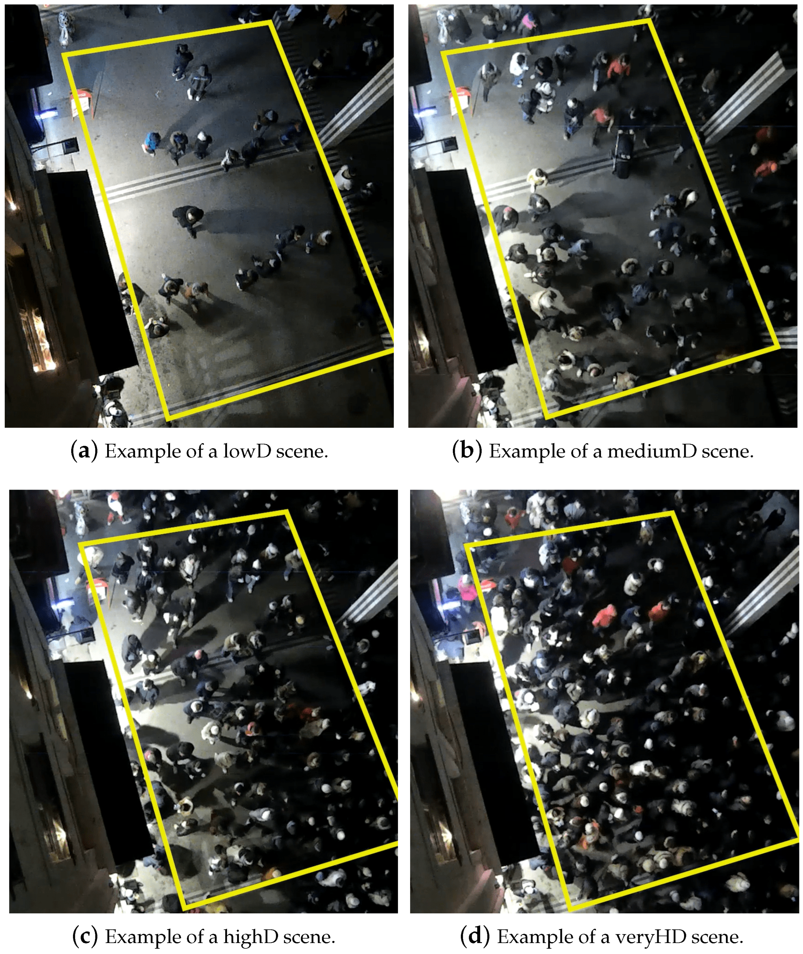
3. The Dataset
4. Methodology
4.1. Overview
4.2. Prediction Approaches
4.2.1. Constant Velocity Model
4.2.2. Social Force Model
4.2.3. Vanilla LSTM
4.2.4. Social LSTM
4.2.5. Social GAN
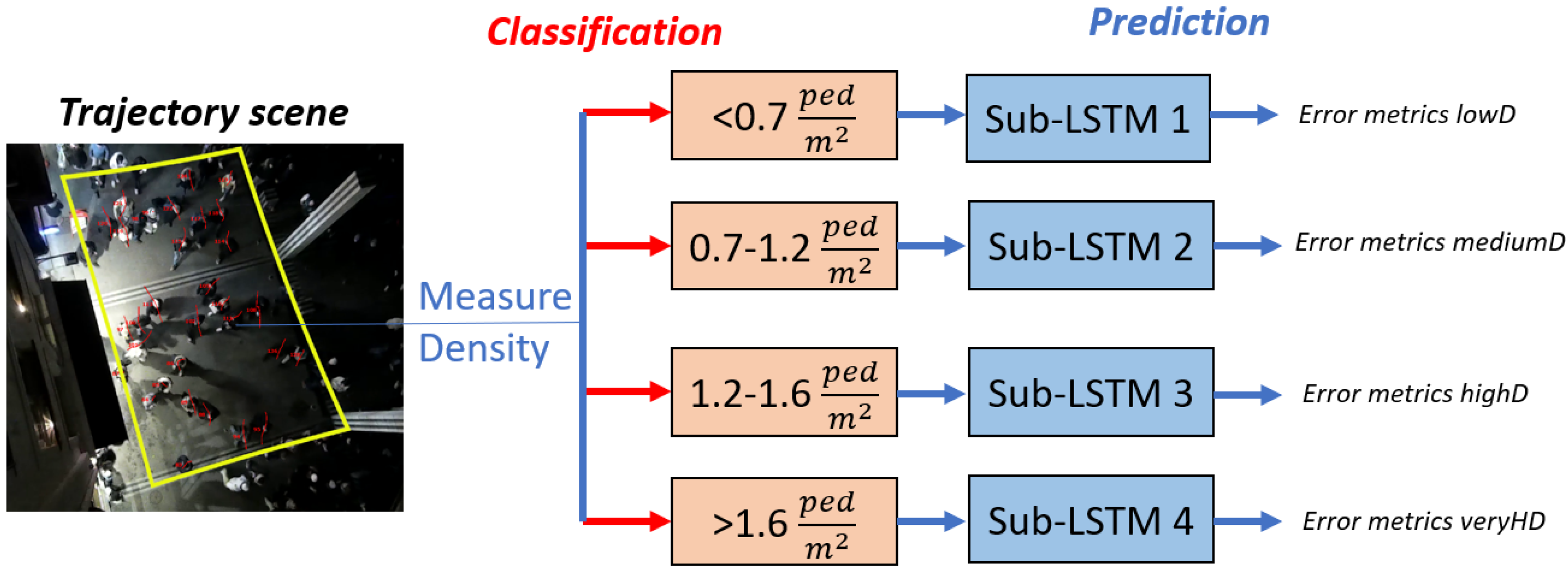
4.3. Two-Stage Process
4.4. Collision Weight
4.5. Implementation Details
5. Results
5.1. Two-Stage Predictions
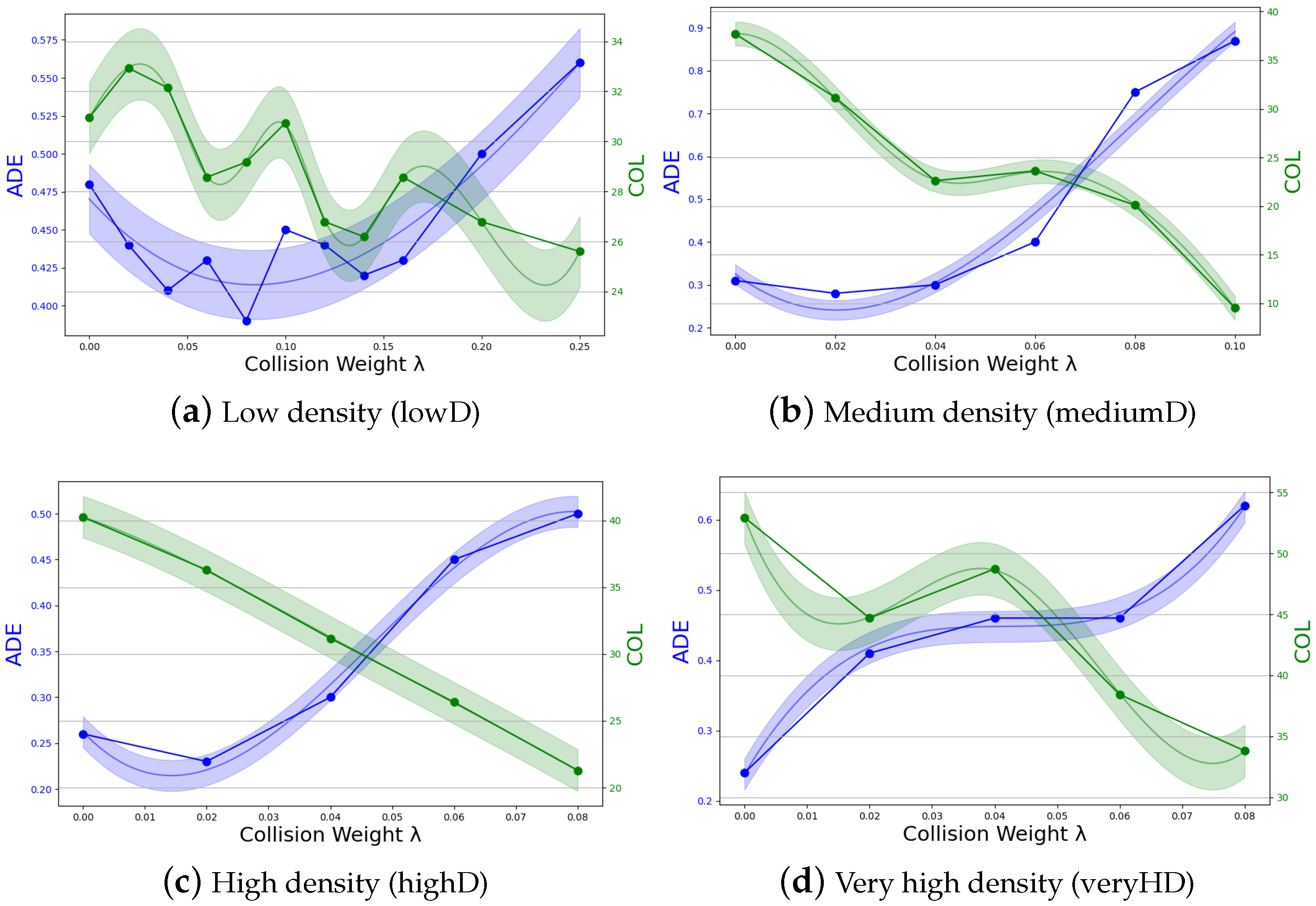
5.2. Collision Weight
6. Conclusions
Author Contributions
Funding
Informed Consent Statement
Data Availability Statement
Acknowledgments
Conflicts of Interest
Abbreviations
| DL | Deep learning |
| PB | Physics-based |
| LSTM | Long Short-Term Memory |
| SLSTM | Social Long Short-Term Memory |
| GAN | Generative Adversarial Network |
| SGAN | Social Generative Adversarial Network |
| TTC | Time-to-collision |
| SF | Social Force model |
| CV | Constant Velocity model |
| ORCA | Optimal Reciprocal Collision Avoidance |
| RNN | Recurrent Neural Network |
| ADE | Average displacement error |
| FDE | Final displacement error |
| COL | Collision metric |
| lowD | Low density |
| mediumD | Medium density |
| highD | High density |
| VeryHD | Very high density |
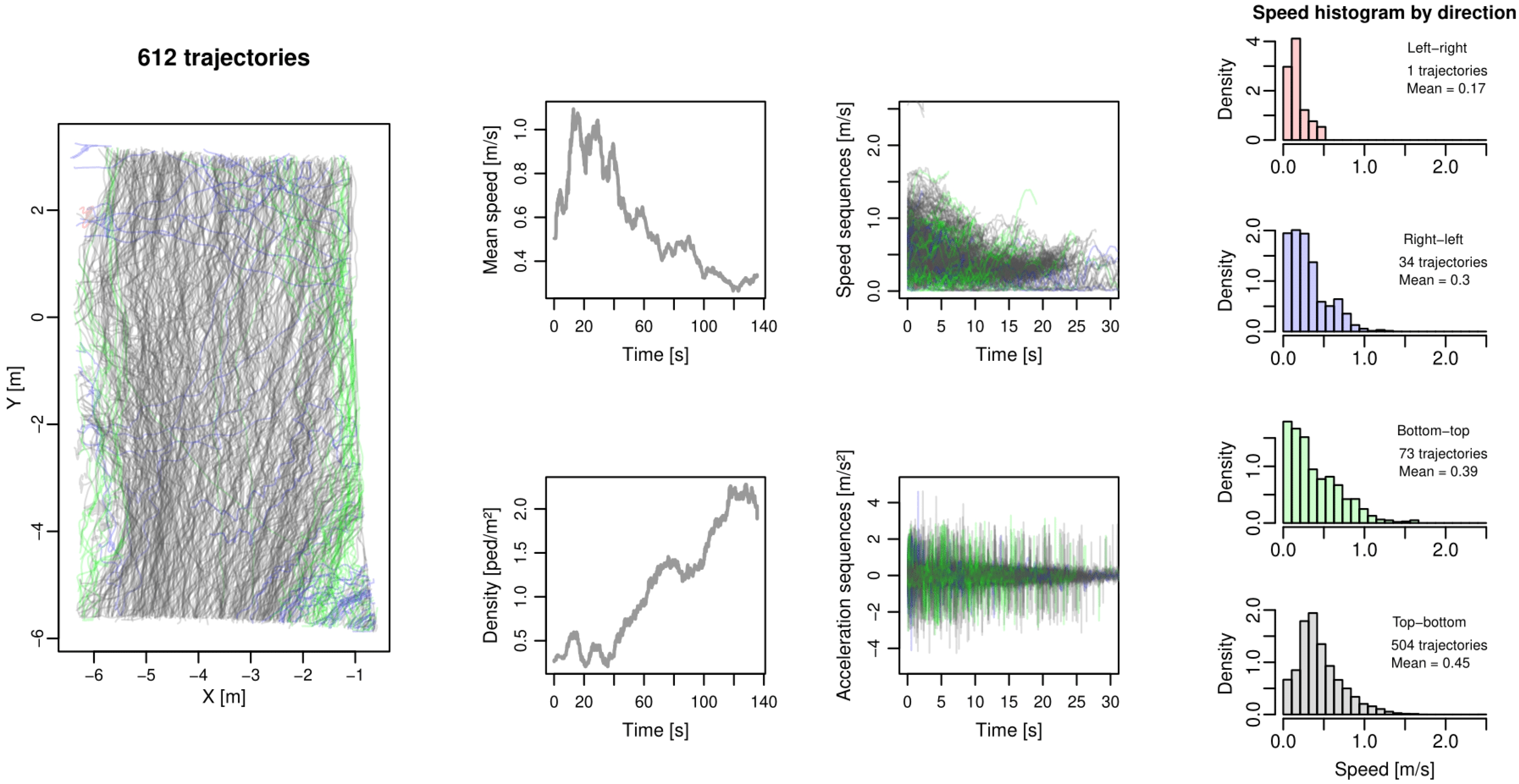
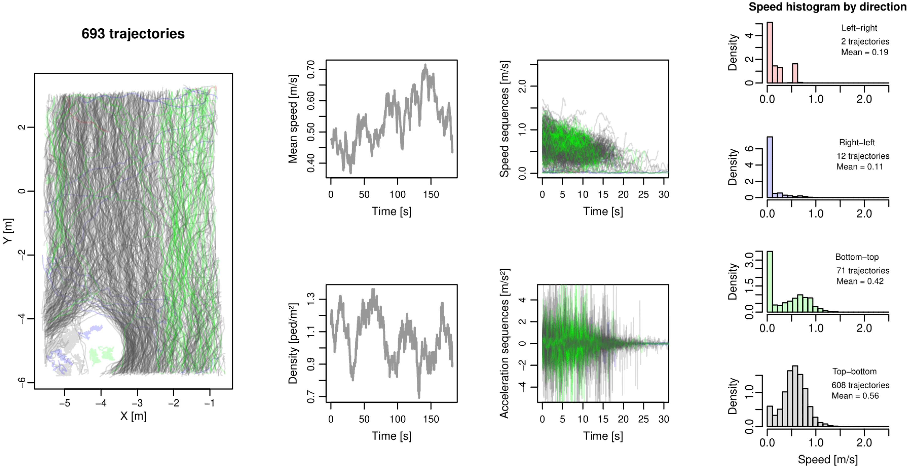
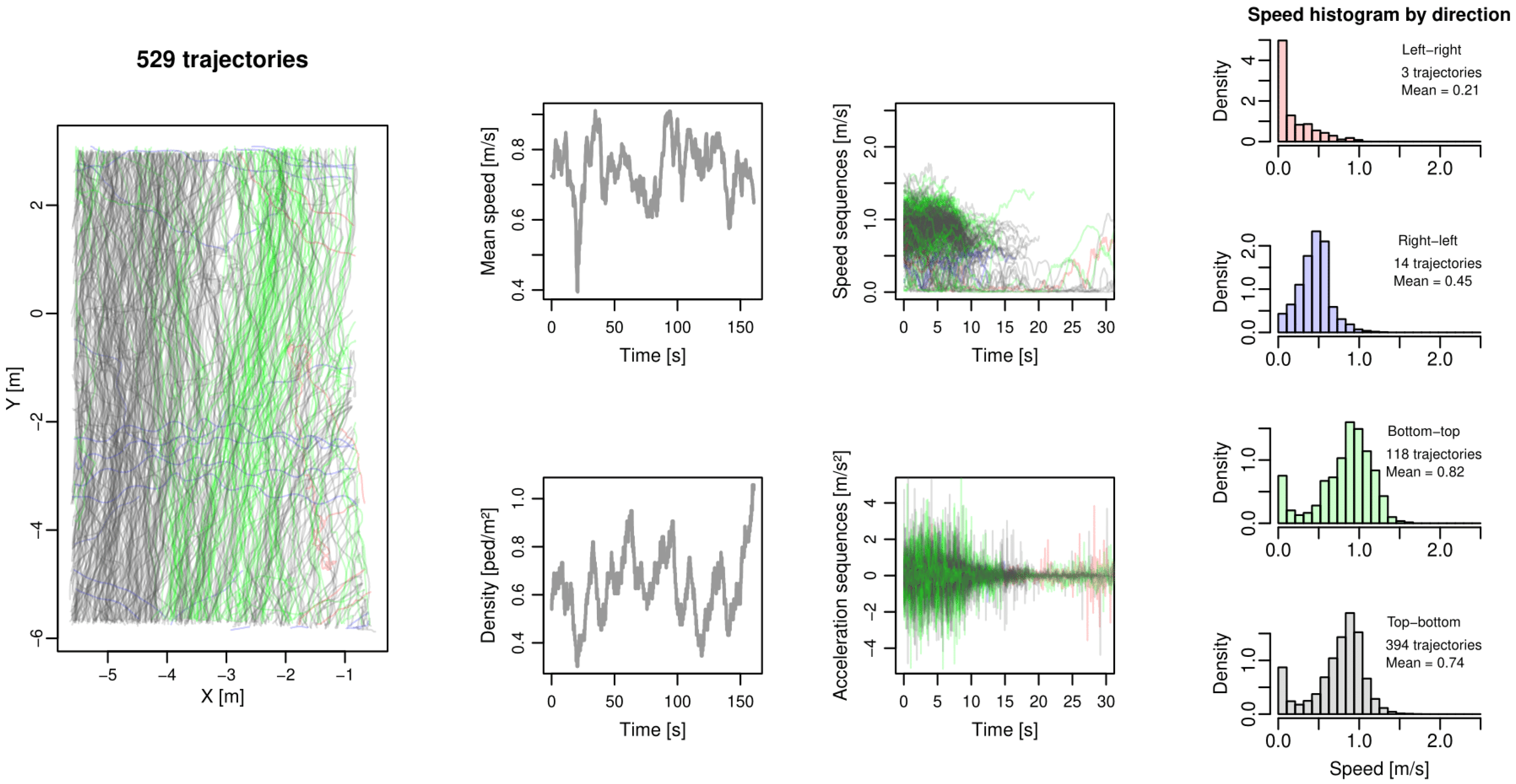
Appendix A
- grey trajectories correspond to pedestrians moving from top to bottom;
- green trajectories for bottom to top;
- blue trajectories for right to left;
- red trajectories for left to right.


References
- Poibrenski, A.; Klusch, M.; Vozniak, I.; Müller, C. M2p3: Multimodal multi-pedestrian path prediction by self-driving cars with egocentric vision. In Proceedings of the 35th Annual ACM Symposium on Applied Computing, Brno, Czech Republic, 30 March–3 April 2020; pp. 190–197. [Google Scholar]
- Scheggi, S.; Aggravi, M.; Morbidi, F.; Prattichizzo, D. Cooperative human–robot haptic navigation. In Proceedings of the 2014 IEEE International Conference on Robotics and Automation (ICRA), Hong Kong, China, 31 May–7 June 2014; pp. 2693–2698. [Google Scholar]
- Boltes, M.; Zhang, J.; Tordeux, A.; Schadschneider, A.; Seyfried, A. Empirical results of pedestrian and evacuation dynamics. Encycl. Complex. Syst. Sci. 2018, 16, 1–29. [Google Scholar]
- Korbmacher, R.; Tordeux, A. Review of pedestrian trajectory prediction methods: Comparing deep learning and knowledge-based approaches. IEEE Trans. Intell. Transp. Syst. 2022, 23, 24126–24144. [Google Scholar] [CrossRef]
- Alahi, A.; Goel, K.; Ramanathan, V.; Robicquet, A.; Li, F.-F.; Savarese, S. Social LSTM: Human trajectory prediction in crowded spaces. In Proceedings of the IEEE Conference on Computer Vision and Pattern Recognition, Las Vegas, NV, USA, 27–30 June 2016; pp. 961–971. [Google Scholar]
- Dang, H.T.; Korbmacher, R.; Tordeux, A.; Gaudou, B.; Verstaevel, N. TTC-SLSTM: Human trajectory prediction using time-to-collision interaction energy. In Proceedings of the 2023 15th International Conference on Knowledge and Systems Engineering (KSE), Hanoi, Vietnam, 18–20 October 2023; pp. 1–6. [Google Scholar]
- Karamouzas, I.; Skinner, B.; Guy, S.J. Universal power law governing pedestrian interactions. Phys. Rev. Lett. 2014, 113, 238701. [Google Scholar] [CrossRef] [PubMed]
- Helbing, D.; Molnar, P. Social force model for pedestrian dynamics. Phys. Rev. E 1995, 51, 4282. [Google Scholar] [CrossRef] [PubMed]
- Van Den Berg, J.; Guy, S.J.; Lin, M.; Manocha, D. Reciprocal n-body collision avoidance. In Robotics Research: The 14th International Symposium ISRR, Lucerne, Switzerland, 31 August–3 September 2009; Springer: Berlin/Heidelberg, Germany, 2011; pp. 3–19. [Google Scholar]
- Burstedde, C.; Klauck, K.; Schadschneider, A.; Zittartz, J. Simulation of pedestrian dynamics using a two-dimensional cellular automaton. Phys. A Stat. Mech. Its Appl. 2001, 295, 507–525. [Google Scholar] [CrossRef]
- Bellomo, N.; Dogbe, C. On the modeling of traffic and crowds: A survey of models, speculations, and perspectives. SIAM Rev. 2011, 53, 409–463. [Google Scholar] [CrossRef]
- Chraibi, M.; Tordeux, A.; Schadschneider, A.; Seyfried, A. Modelling of pedestrian and evacuation dynamics. In Encyclopedia of Complexity and Systems Science; Springer: Berlin/Heidelberg, Germany, 2018; pp. 1–22. [Google Scholar]
- Duives, D.C.; Daamen, W.; Hoogendoorn, S.P. State-of-the-art crowd motion simulation models. Transp. Res. Part C Emerg. Technol. 2013, 37, 193–209. [Google Scholar] [CrossRef]
- Gupta, A.; Johnson, J.; Li, F.-F.; Savarese, S.; Alahi, A. Social GAN: Socially acceptable trajectories with generative adversarial networks. In Proceedings of the IEEE Conference on Computer Vision and Pattern Recognition, Salt Lake City, UT, USA, 18–23 June 2018; pp. 2255–2264. [Google Scholar]
- Vemula, A.; Muelling, K.; Oh, J. Social attention: Modeling attention in human crowds. In Proceedings of the 2018 IEEE International Conference on Robotics and Automation (ICRA), Brisbane, QLD, Australia, 21–25 May 2018; pp. 4601–4607. [Google Scholar]
- Monti, A.; Bertugli, A.; Calderara, S.; Cucchiara, R. Dag-net: Double attentive graph neural network for trajectory forecasting. In Proceedings of the 2020 25th International Conference on Pattern Recognition (ICPR), Milan, Italy, 10–15 January 2021; pp. 2551–2558. [Google Scholar]
- Shi, X.; Shao, X.; Guo, Z.; Wu, G.; Zhang, H.; Shibasaki, R. Pedestrian trajectory prediction in extremely crowded scenarios. Sensors 2019, 19, 1223. [Google Scholar] [CrossRef] [PubMed]
- Yi, S.; Li, H.; Wang, X. Pedestrian behavior understanding and prediction with deep neural networks. In Proceedings of the Computer Vision—ECCV 2016: 14th European Conference, Amsterdam, The Netherlands, 11–14 October 2016; Springer: Berlin/Heidelberg, Germany, 2016; pp. 263–279. [Google Scholar]
- Li, Y.; Xu, H.; Bian, M.; Xiao, J. Attention based CNN-ConvLSTM for pedestrian attribute recognition. Sensors 2020, 20, 811. [Google Scholar] [CrossRef]
- Yao, H.Y.; Wan, W.G.; Li, X. End-to-end pedestrian trajectory forecasting with transformer network. ISPRS Int. J. Geo-Inf. 2022, 11, 44. [Google Scholar] [CrossRef]
- Xue, H.; Huynh, D.Q.; Reynolds, M. Bi-prediction: Pedestrian trajectory prediction based on bidirectional LSTM classification. In Proceedings of the 2017 International Conference on Digital Image Computing: Techniques and Applications (DICTA), Sydney, NSW, Australia, 29 November–1 December 2017; pp. 1–8. [Google Scholar]
- Xue, H.; Huynh, D.Q.; Reynolds, M. PoPPL: Pedestrian trajectory prediction by LSTM with automatic route class clustering. IEEE Trans. Neural Netw. Learn. Syst. 2020, 32, 77–90. [Google Scholar] [CrossRef]
- Kothari, P.; Kreiss, S.; Alahi, A. Human trajectory forecasting in crowds: A deep learning perspective. IEEE Trans. Intell. Transp. Syst. 2021, 23, 7386–7400. [Google Scholar] [CrossRef]
- Papathanasopoulou, V.; Spyropoulou, I.; Perakis, H.; Gikas, V.; Andrikopoulou, E. A data-driven model for pedestrian behavior classification and trajectory prediction. IEEE Open J. Intell. Transp. Syst. 2022, 3, 328–339. [Google Scholar] [CrossRef]
- Khadka, A.; Remagnino, P.; Argyriou, V. Synthetic crowd and pedestrian generator for deep learning problems. In Proceedings of the ICASSP 2020—2020 IEEE International Conference on Acoustics, Speech and Signal Processing (ICASSP), Barcelona, Spain, 4–8 May 2020; pp. 4052–4056. [Google Scholar]
- Antonucci, A.; Papini, G.P.R.; Bevilacqua, P.; Palopoli, L.; Fontanelli, D. Efficient prediction of human motion for real-time robotics applications with physics-inspired neural networks. IEEE Access 2021, 10, 144–157. [Google Scholar] [CrossRef]
- Silvestri, M.; Lombardi, M.; Milano, M. Injecting domain knowledge in neural networks: A controlled experiment on a constrained problem. In Proceedings of the Integration of Constraint Programming, Artificial Intelligence, and Operations Research: 18th International Conference, CPAIOR 2021, Vienna, Austria, 5–8 July 2021; Springer: Berlin/Heidelberg, Germany, 2021; pp. 266–282. [Google Scholar]
- Kothari, P.; Alahi, A. Safety-compliant generative adversarial networks for human trajectory forecasting. IEEE Trans. Intell. Transp. Syst. 2023, 24, 4251–4261. [Google Scholar] [CrossRef]
- Pellegrini, S.; Ess, A.; Schindler, K.; Van Gool, L. You’ll never walk alone: Modeling social behavior for multi-target tracking. In Proceedings of the 2009 IEEE 12th International Conference on Computer Vision, Kyoto, Japan, 27 September–4 October 2009; pp. 261–268. [Google Scholar]
- Lerner, A.; Chrysanthou, Y.; Lischinski, D. Crowds by example. In Computer Graphics Forum; Wiley Online Library: Hoboken, NJ, USA, 2007; Volume 26, pp. 655–664. [Google Scholar]
- Gabbana, A.; Toschi, F.; Ross, P.; Haans, A.; Corbetta, A. Fluctuations in pedestrian dynamics routing choices. PNAS Nexus 2022, 1, pgac169. [Google Scholar] [CrossRef] [PubMed]
- Robicquet, A.; Sadeghian, A.; Alahi, A.; Savarese, S. Learning social etiquette: Human trajectory understanding in crowded scenes. In Proceedings of the Computer Vision—ECCV 2016: 14th European Conference, Amsterdam, The Netherlands, 11–14 October 2016; Springer: Berlin/Heidelberg, Germany, 2016; pp. 549–565. [Google Scholar]
- Zhou, B.; Wang, X.; Tang, X. Understanding collective crowd behaviors: Learning a mixture model of dynamic pedestrian-agents. In Proceedings of the 2012 IEEE Conference on Computer Vision and Pattern Recognition, Providence, RI, USA, 16–21 June 2012; pp. 2871–2878. [Google Scholar]
- Majecka, B. Statistical Models of Pedestrian Behaviour in the Forum. Master’s Thesis, University of Edinburgh, Edinburgh, UK, 2009. [Google Scholar]
- Boltes, M.; Seyfried, A. Collecting pedestrian trajectories. Neurocomputing 2013, 100, 127–133. [Google Scholar] [CrossRef]
- Korbmacher, R.; Dang, H.T.; Tordeux, A. Predicting pedestrian trajectories at different densities: A multi-criteria empirical analysis. Phys. A Stat. Mech. Its Appl. 2024, 634, 129440. [Google Scholar] [CrossRef]
- Hochreiter, S.; Schmidhuber, J. Long short-term memory. Neural Comput. 1997, 9, 1735–1780. [Google Scholar] [CrossRef]
- Korbmacher, R.; Dang-Huu, T.; Tordeux, A.; Verstaevel, N.; Gaudou, B. Differences in pedestrian trajectory predictions for high-and low-density situations. In Proceedings of the 14th International Conference on Traffic and Granular Flow (TGF) 2022, New Delhi, India, 15–17 October 2022. [Google Scholar]
- Goodfellow, I.; Pouget-Abadie, J.; Mirza, M.; Xu, B.; Warde-Farley, D.; Ozair, S.; Courville, A.; Bengio, Y. Generative adversarial nets. Adv. Neural Inf. Process. Syst. 2014, 27, 2672–2680. [Google Scholar]
- Holl, S. Methoden für die Bemessung der Leistungsfähigkeit Multidirektional Genutzter Fußverkehrsanlagen; FZJ-2017-00069; Jülich Supercomputing Center: Jülich, Germany, 2016. [Google Scholar]
- Wirth, T.D.; Dachner, G.C.; Rio, K.W.; Warren, W.H. Is the neighborhood of interaction in human crowds metric, topological, or visual? PNAS Nexus 2023, 2, pgad118. [Google Scholar] [CrossRef] [PubMed]


| Model | LowD | MediumD | HighD | VeryHD | ||||
|---|---|---|---|---|---|---|---|---|
| ADE/FDE | COL | ADE/FDE | COL | ADE/FDE | COL | ADE/FDE | COL | |
| CV | 0.71/0.97 | 54.76 | 0.85/0.98 | 45.73 | 0.53/0.8 | 62.35 | 0.44/0.67 | 81.74 |
| Social Force [8] | 0.78/1.33 | 24.4 | 0.55/0.89 | 31.16 | 0.5/0.82 | 36.43 | 0.36/0.63 | 54.78 |
| Vanilla LSTM | 0.5/0.99 | 31.55 | 0.33/0.63 | 37.69 | 0.29/0.52 | 36.43 | 0.24/0.41 | 63.8 |
| Social LSTM [5] | 0.53/1.02 | 57.74 | 0.37/0.73 | 59.3 | 0.41/0.78 | 64.26 | 0.35/0.66 | 75.37 |
| Social GAN [14] | 0.53/0.99 | 31.36 | 0.39/0.72 | 32.16 | 0.36/0.61 | 32.33 | 0.25/0.41 | 55.94 |
| Our 2stg. SLSTM | 0.48/0.93 | 30.95 | 0.3/0.63 | 36.18 | 0.26/0.4 | 42.02 | 0.24/0.41 | 52.23 |
| Our 2stg. SGAN | 0.44/0.83 | 32.74 | 0.27/0.52 | 40.2 | 0.28/0.5 | 35.33 | 0.26/0.43 | 58.6 |
| Our 2stg. TTC-SLSTM | 0.39/0.73 | 29.17 | 0.3/0.62 | 22.61 | 0.23/0.36 | 36.29 | 0.24/0.41 | 52.23 |
Disclaimer/Publisher’s Note: The statements, opinions and data contained in all publications are solely those of the individual author(s) and contributor(s) and not of MDPI and/or the editor(s). MDPI and/or the editor(s) disclaim responsibility for any injury to people or property resulting from any ideas, methods, instructions or products referred to in the content. |
© 2024 by the authors. Licensee MDPI, Basel, Switzerland. This article is an open access article distributed under the terms and conditions of the Creative Commons Attribution (CC BY) license (https://creativecommons.org/licenses/by/4.0/).
Share and Cite
Korbmacher, R.; Tordeux, A. Toward Better Pedestrian Trajectory Predictions: The Role of Density and Time-to-Collision in Hybrid Deep-Learning Algorithms. Sensors 2024, 24, 2356. https://doi.org/10.3390/s24072356
Korbmacher R, Tordeux A. Toward Better Pedestrian Trajectory Predictions: The Role of Density and Time-to-Collision in Hybrid Deep-Learning Algorithms. Sensors. 2024; 24(7):2356. https://doi.org/10.3390/s24072356
Chicago/Turabian StyleKorbmacher, Raphael, and Antoine Tordeux. 2024. "Toward Better Pedestrian Trajectory Predictions: The Role of Density and Time-to-Collision in Hybrid Deep-Learning Algorithms" Sensors 24, no. 7: 2356. https://doi.org/10.3390/s24072356
APA StyleKorbmacher, R., & Tordeux, A. (2024). Toward Better Pedestrian Trajectory Predictions: The Role of Density and Time-to-Collision in Hybrid Deep-Learning Algorithms. Sensors, 24(7), 2356. https://doi.org/10.3390/s24072356