
Application of Artificial Intelligence and Sensor Fusion for Soil Organic Matter Prediction


Abstract
1. Introduction
2. Methodology
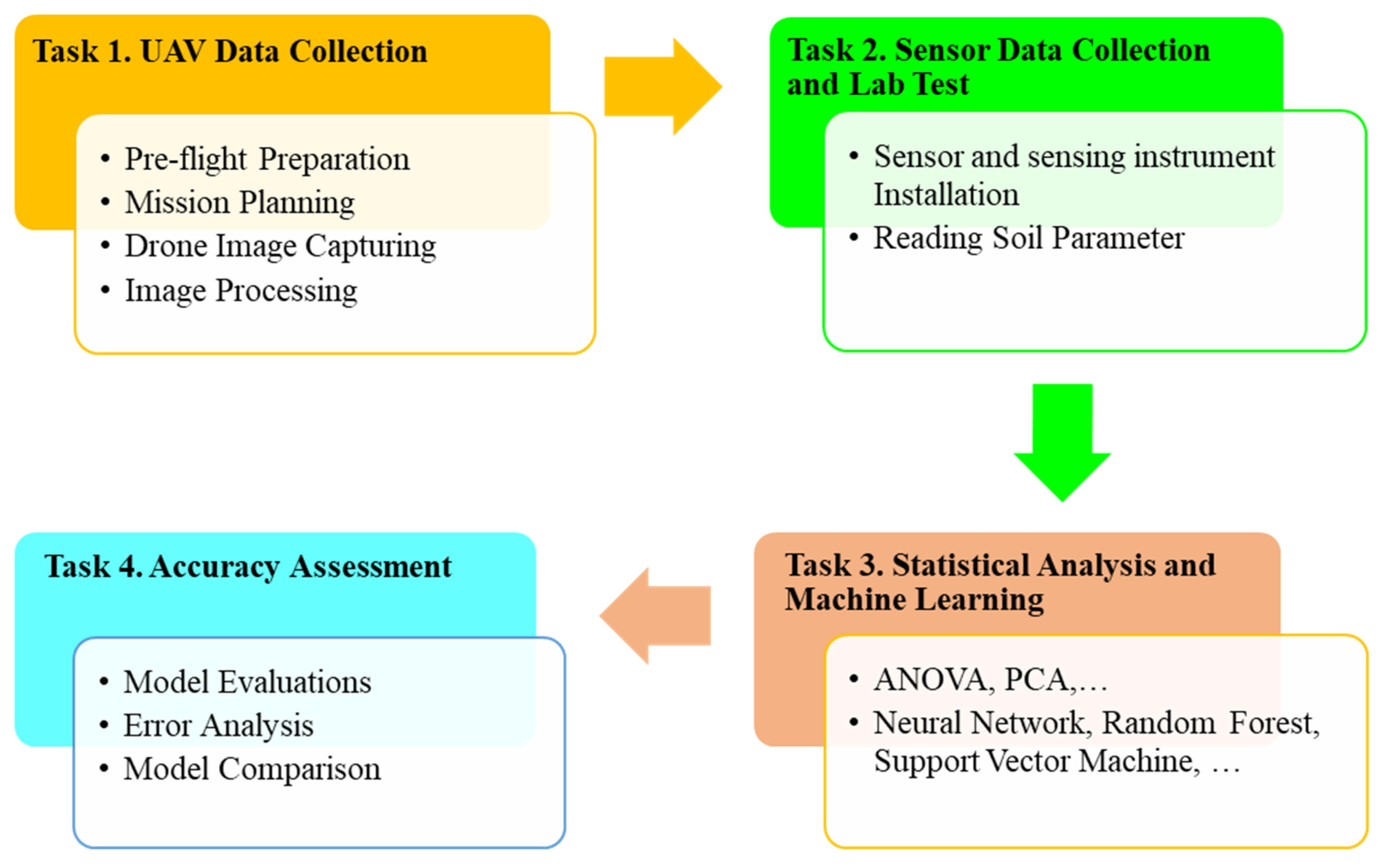
2.1. Research Design
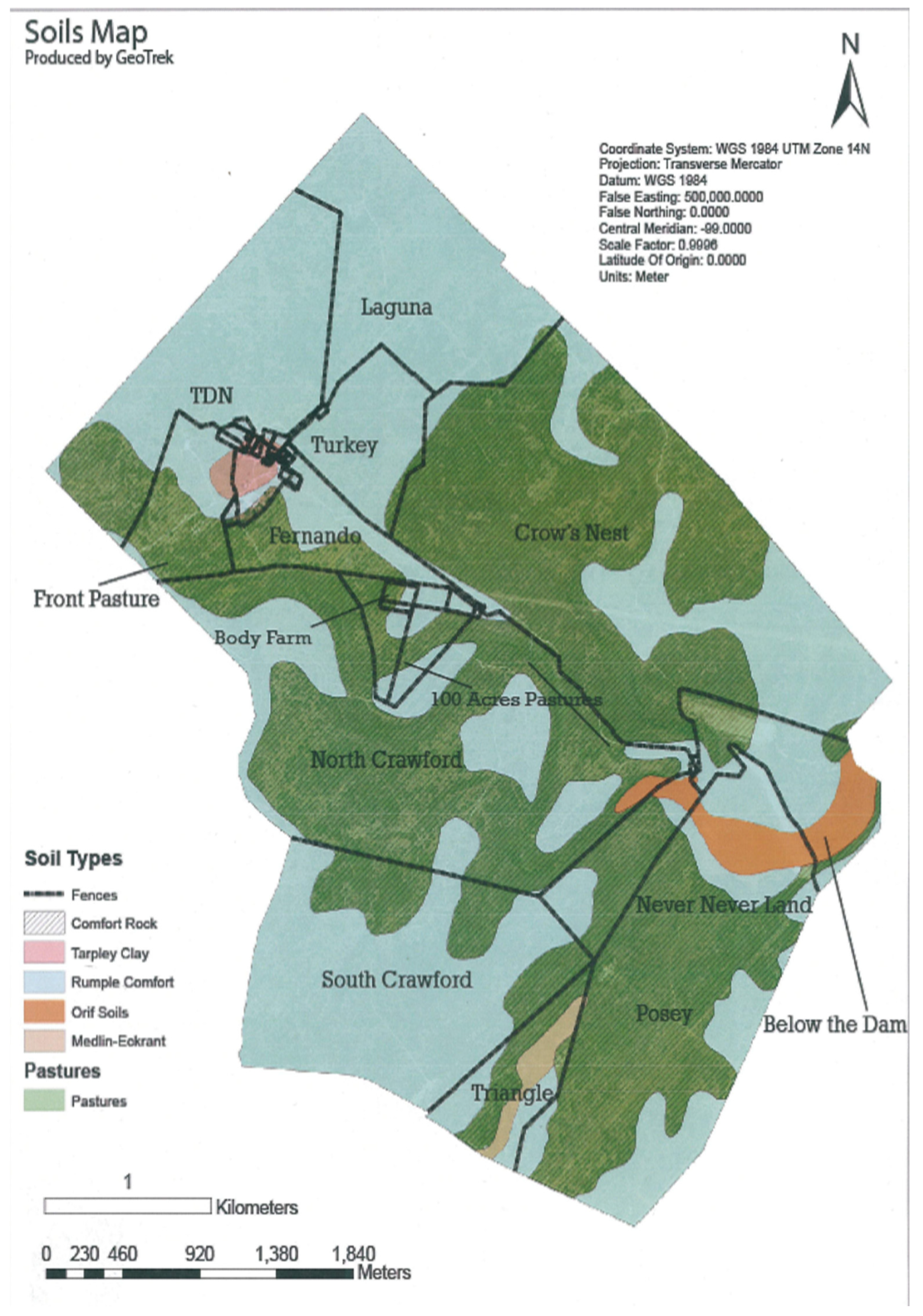
2.2. Research Sites
2.3. Sensor Installation and Soil Parameter Measurement
2.4. Data Analysis
3. Results
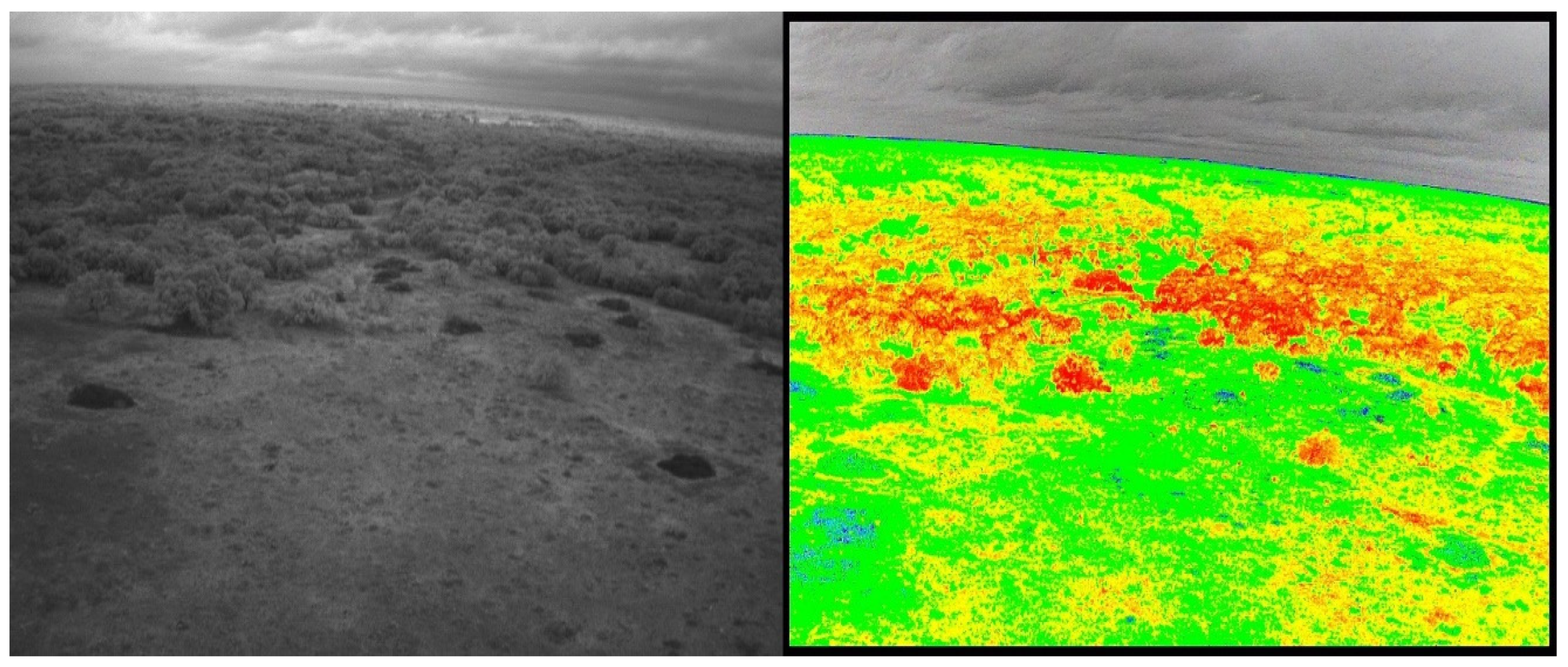
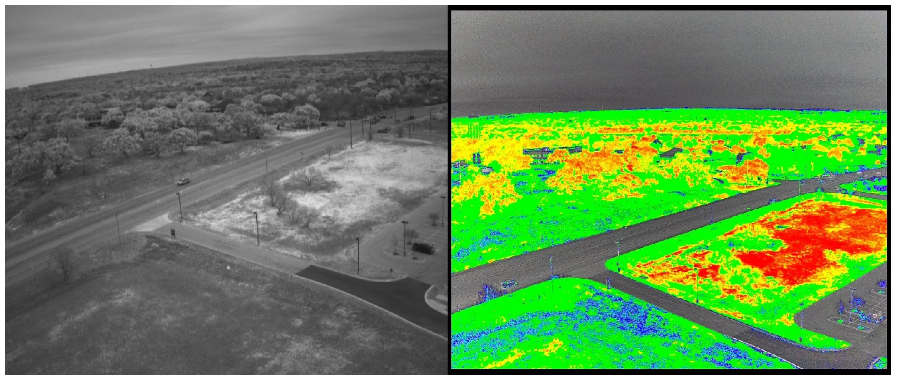
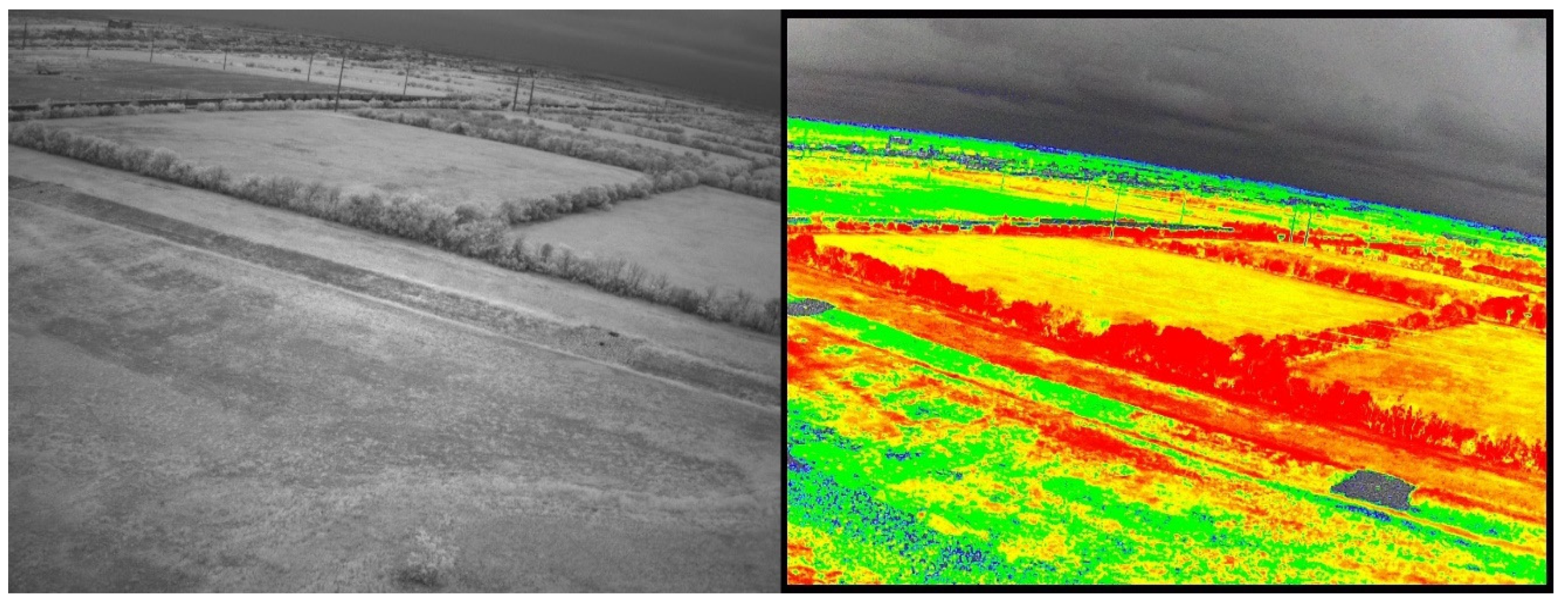
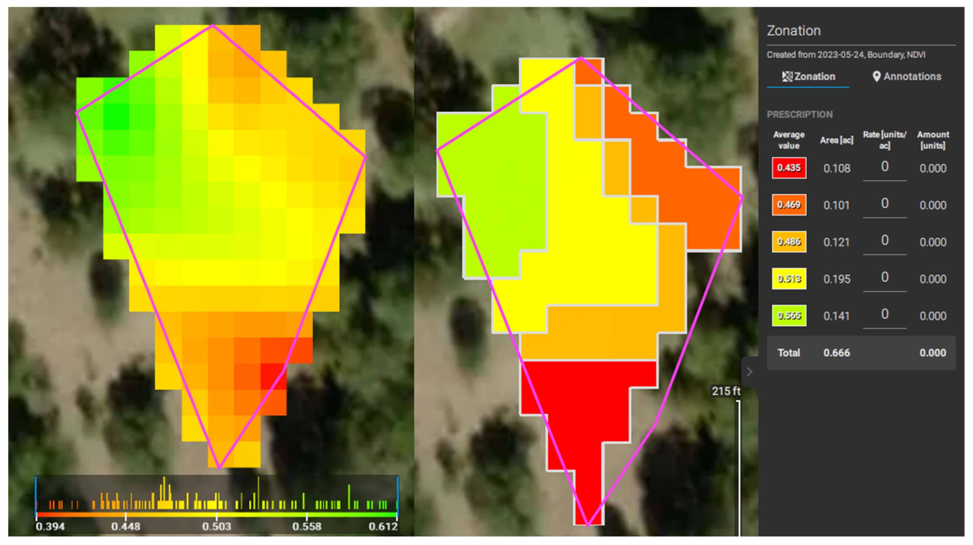
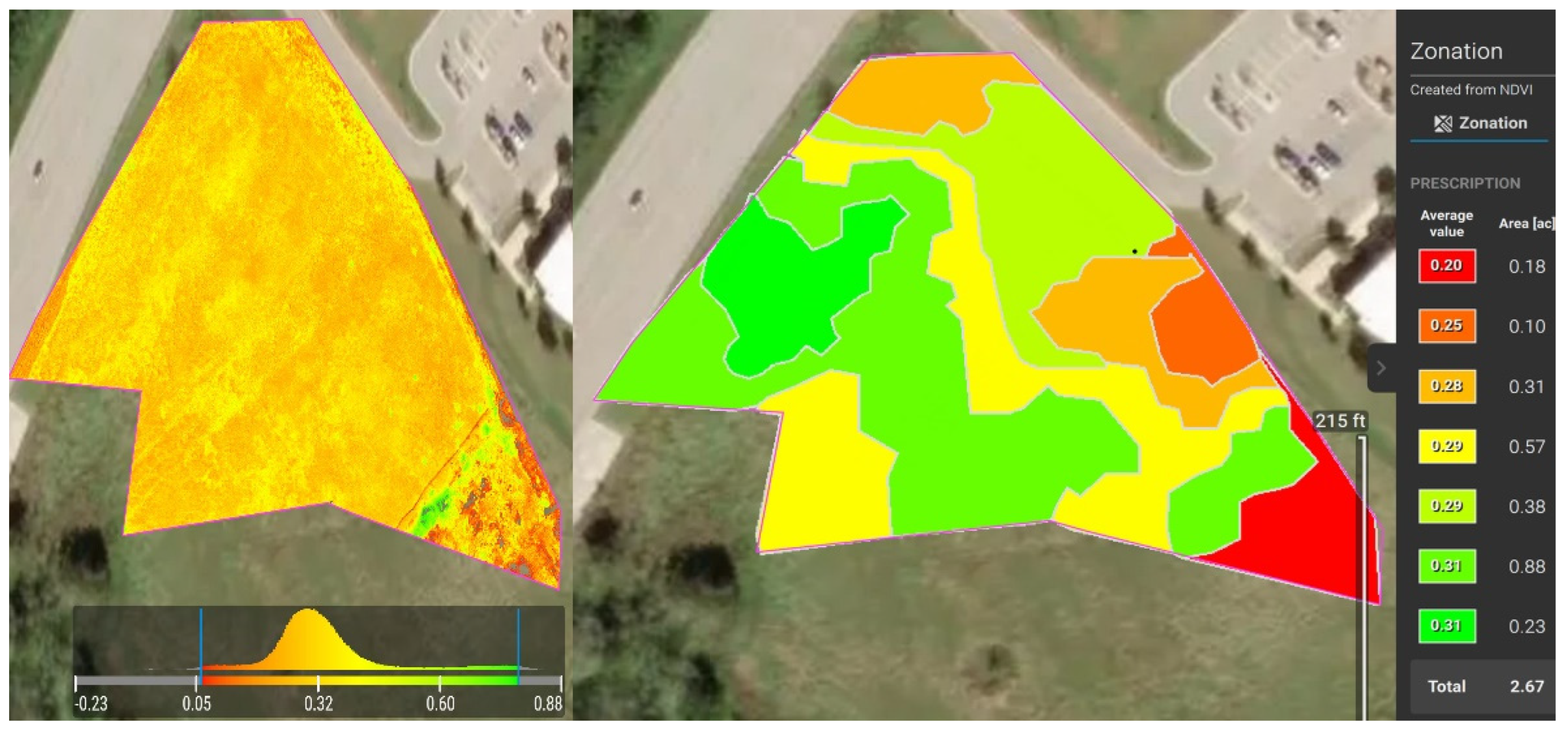
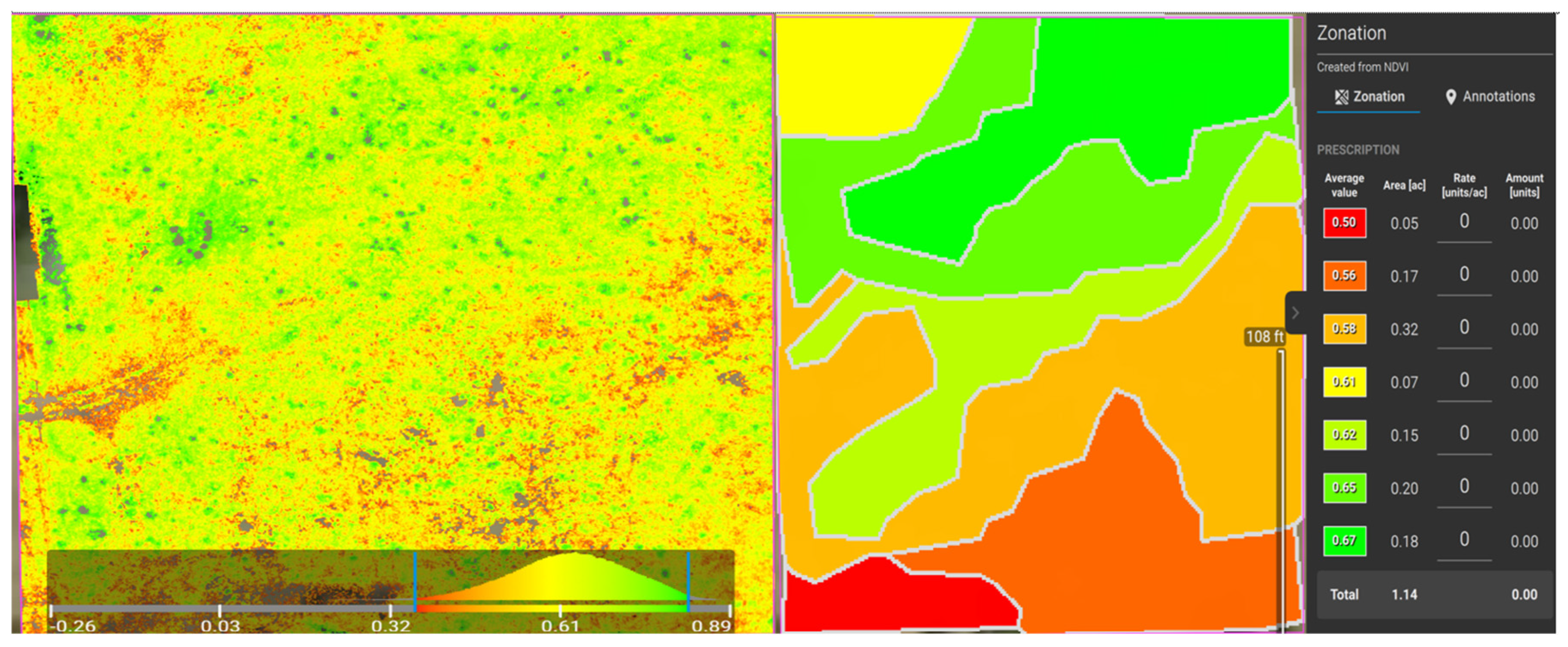
3.1. UAV Survey
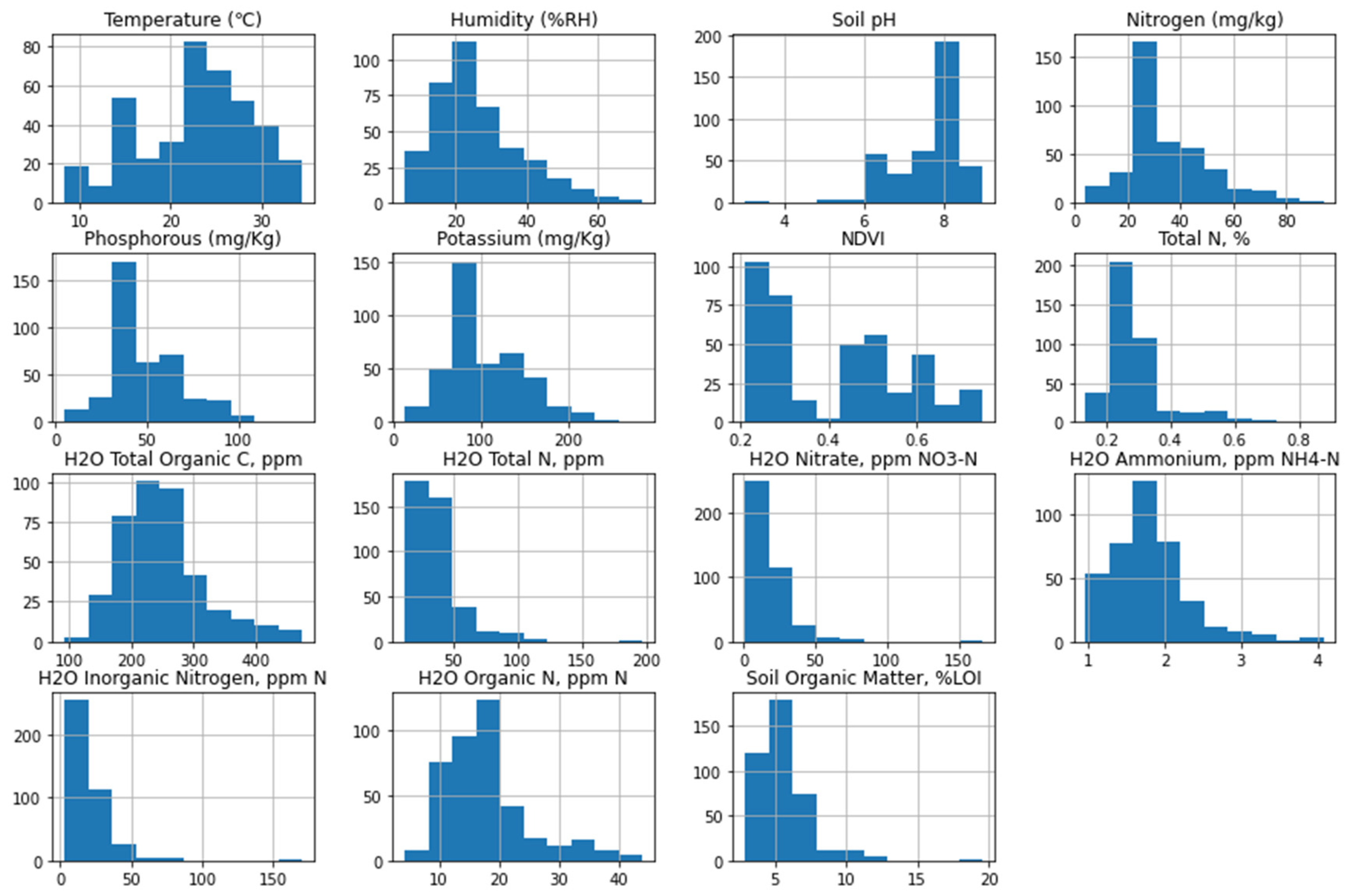
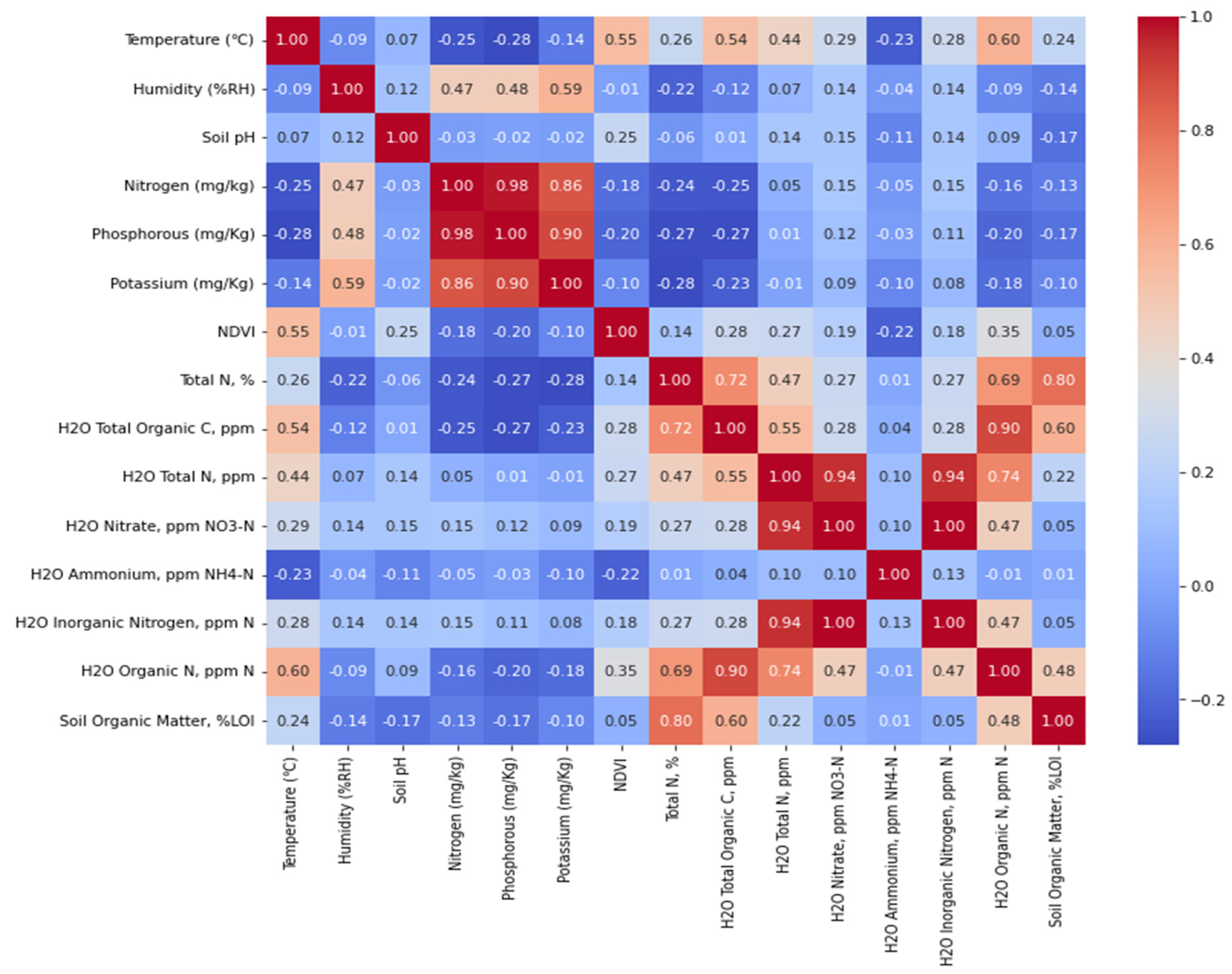
3.2. Results of Data Analysis
3.2.1. Regression Analysis
| Soil Organic Matter, %LOI | = 0.254 + 0.0471 Temperature (°C) − 0.00296 Humidity (%RH) − 0.0818 Soil pH + 0.0771 Nitrogen (mg/kg) − 0.0749 Phosphorous (mg/kg) + 0.01457 Potassium (mg/kg) − 0.926 NDVI + 16.387 Total N (%) |
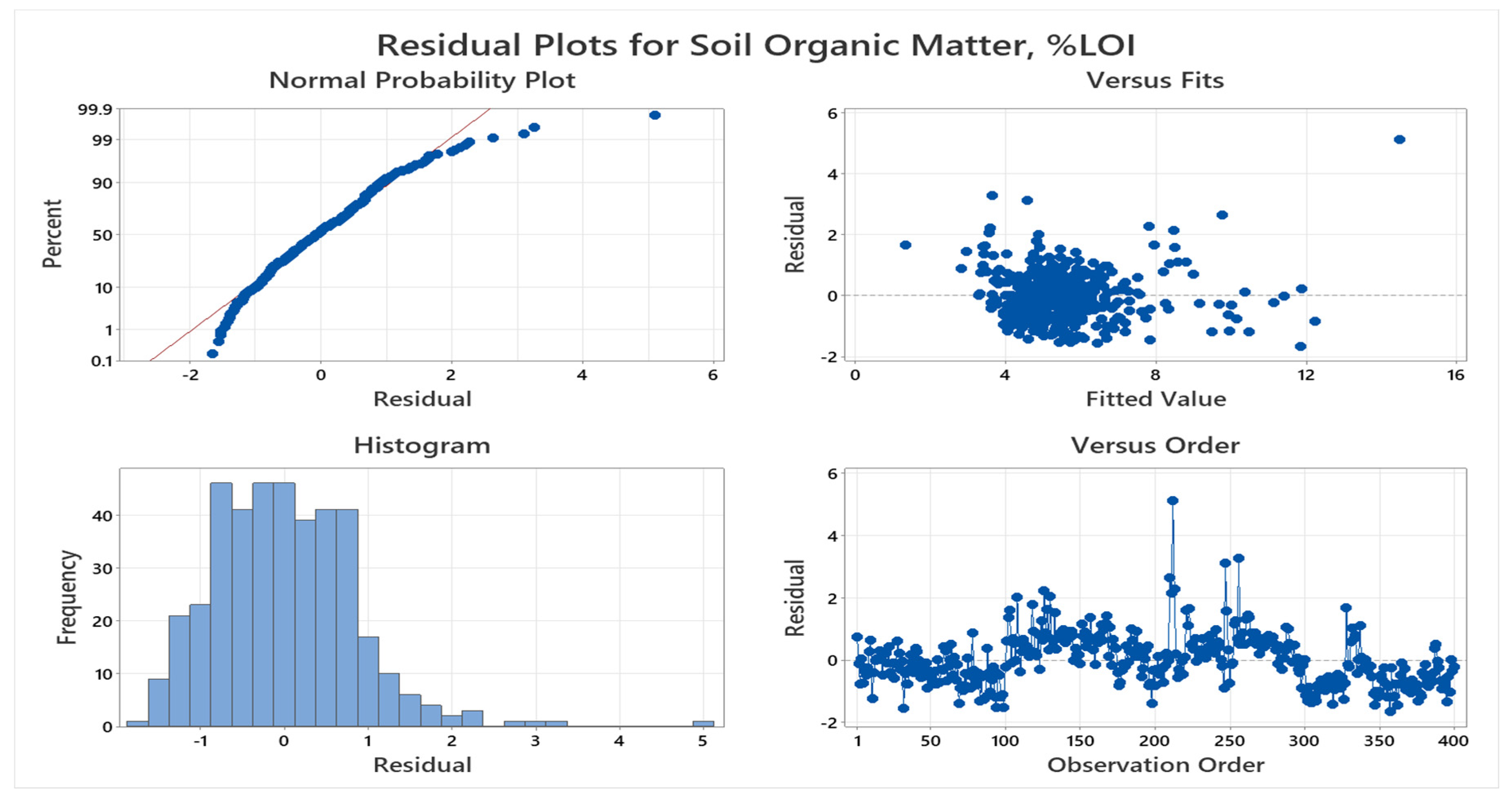
3.2.2. ANOVA Analysis
- Condition (1): Linearity
- Condition (2): Nearly Normal Residuals
- Condition (3): Constant Variability
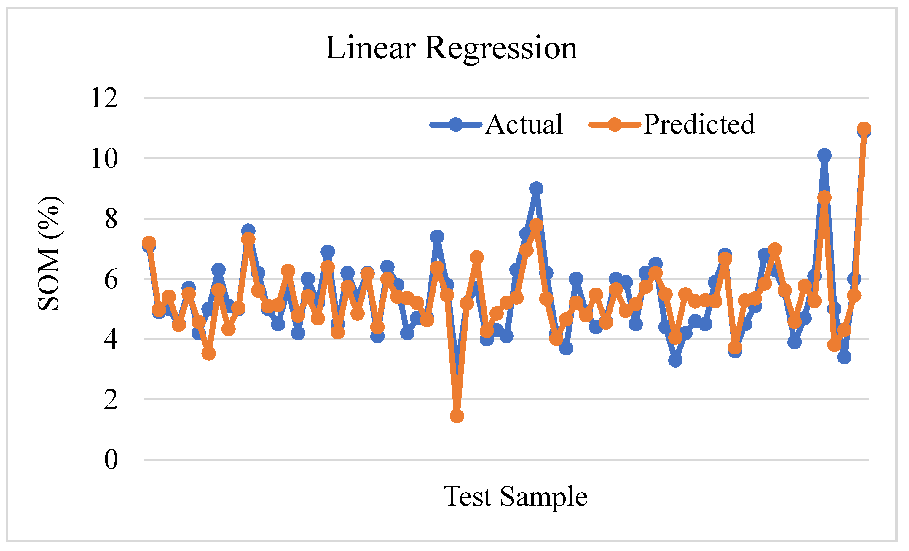
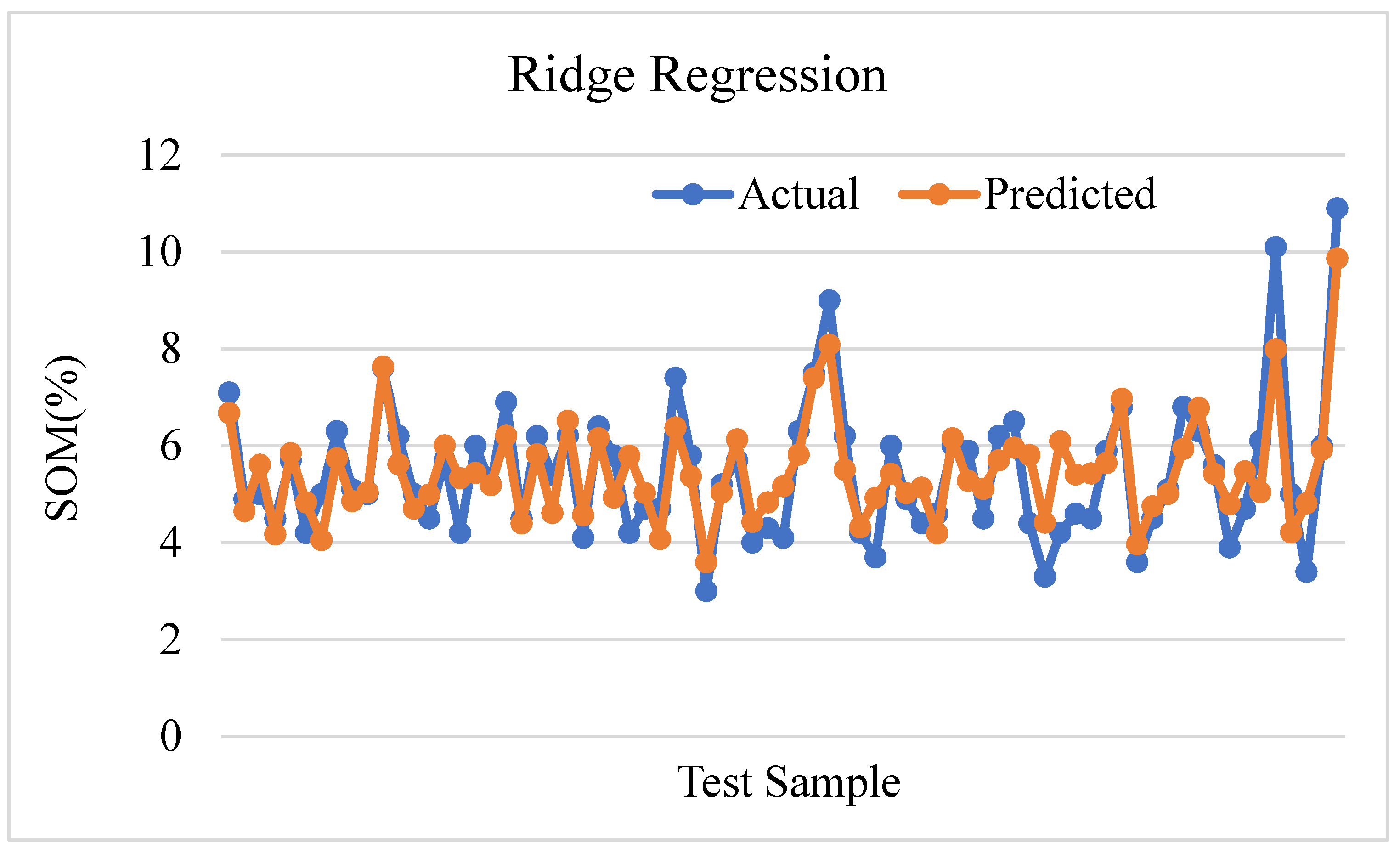
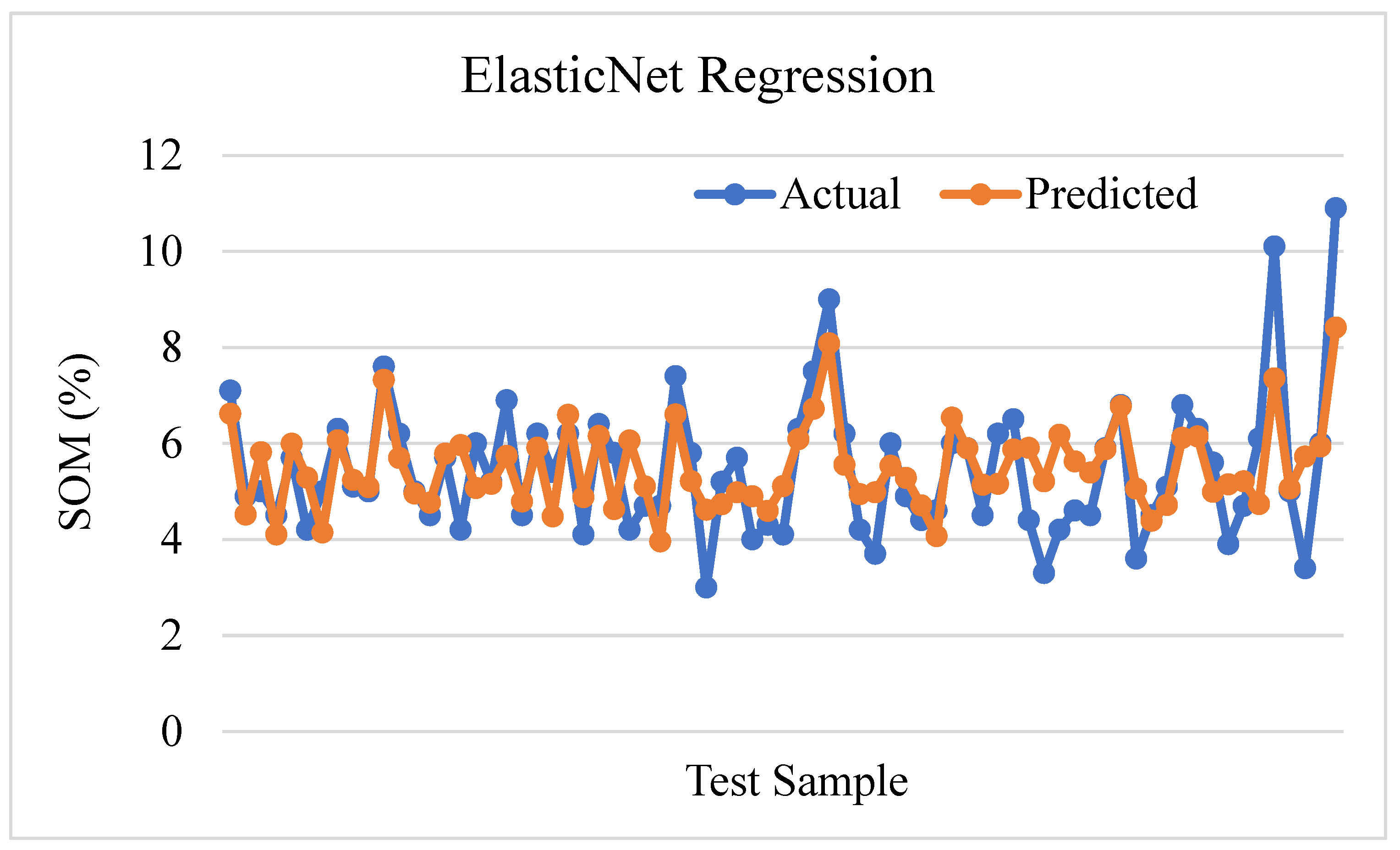
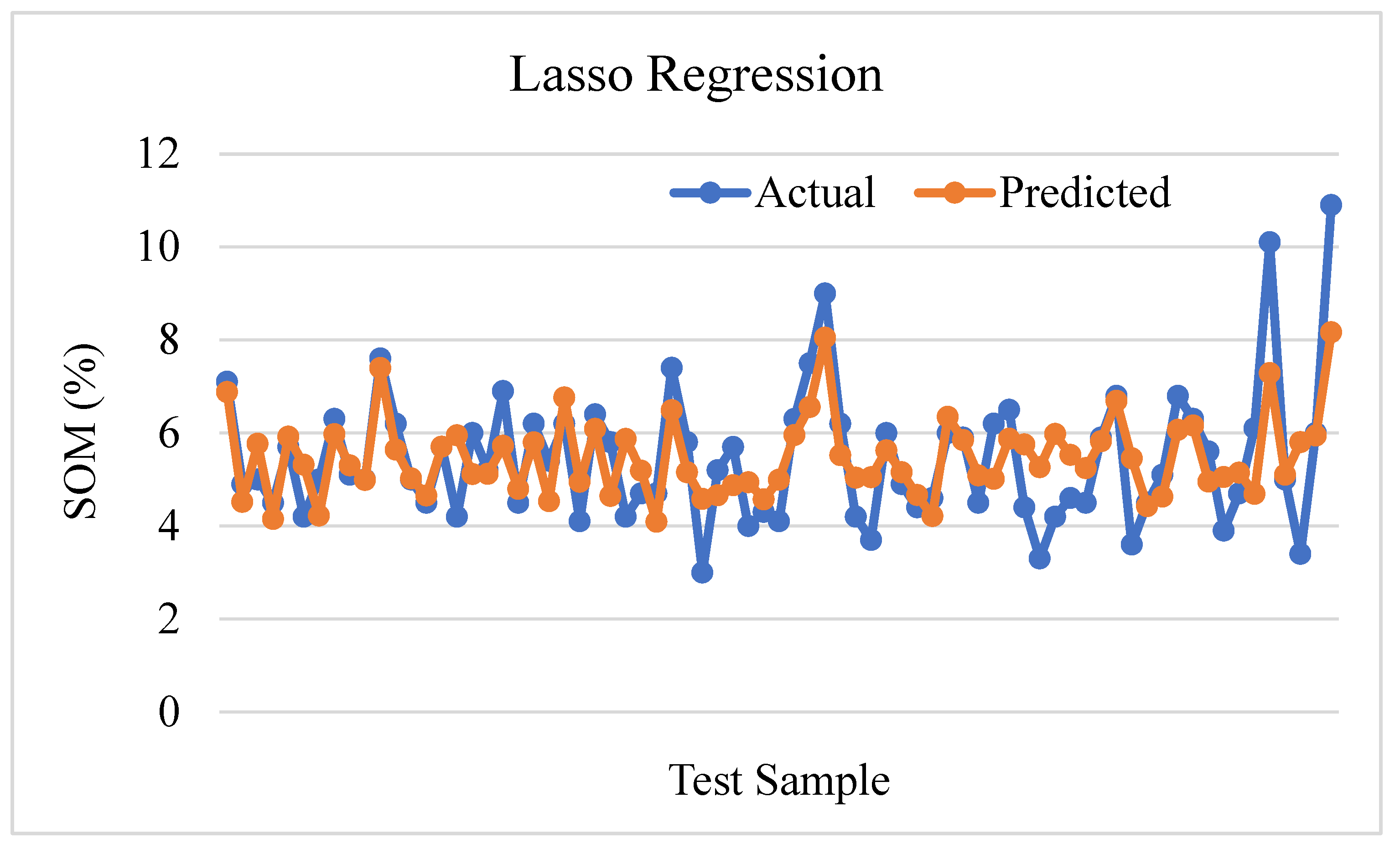
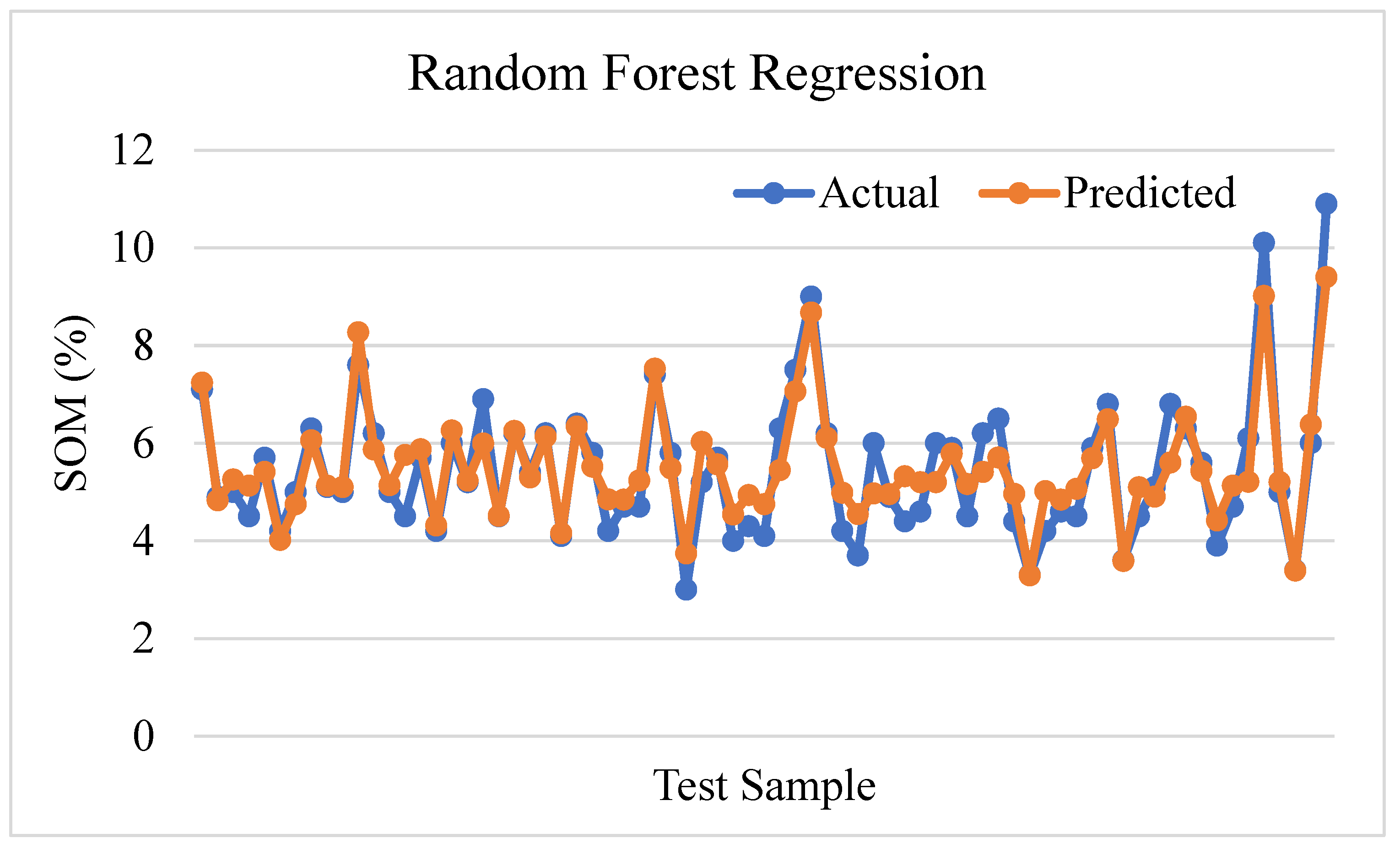
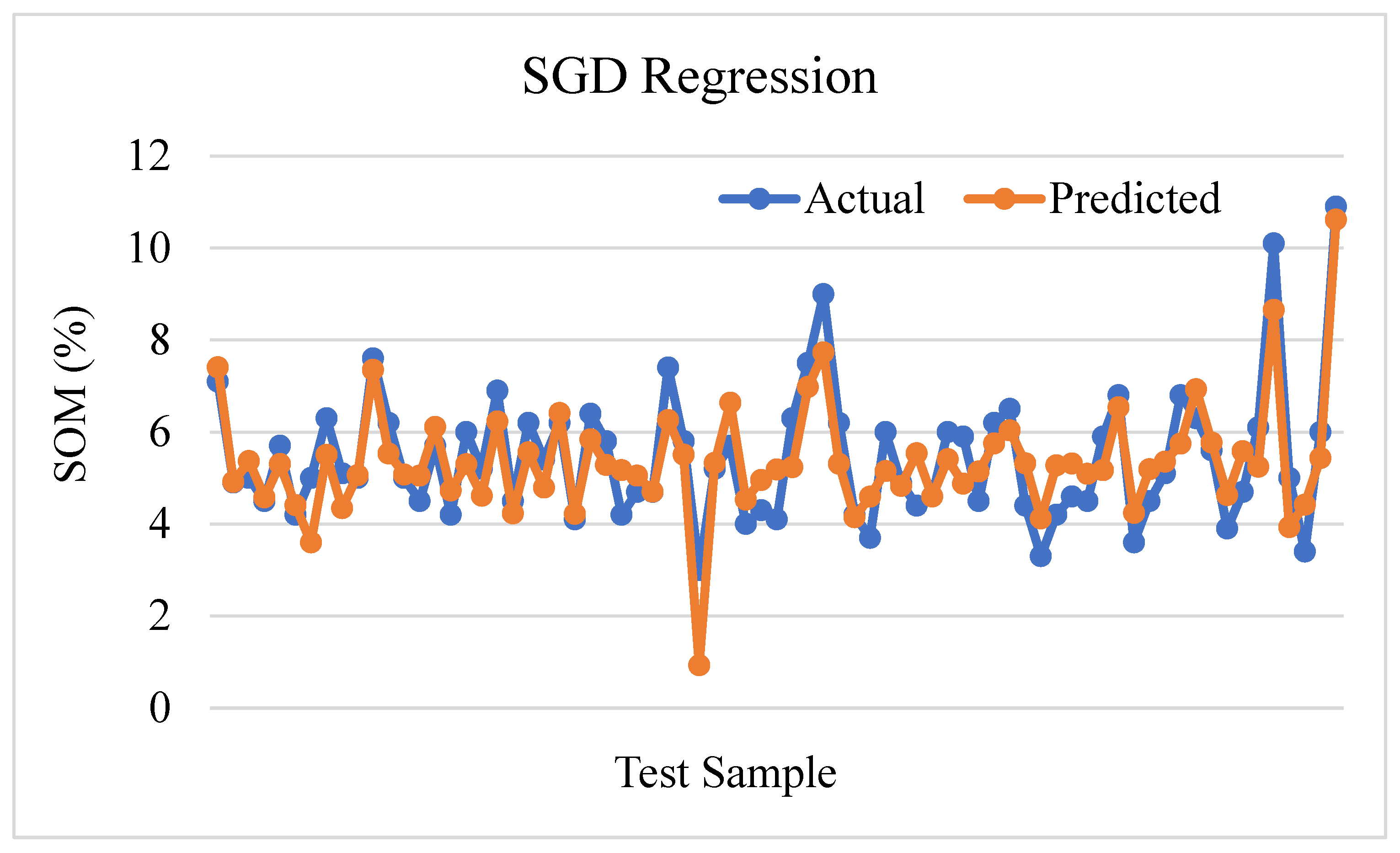
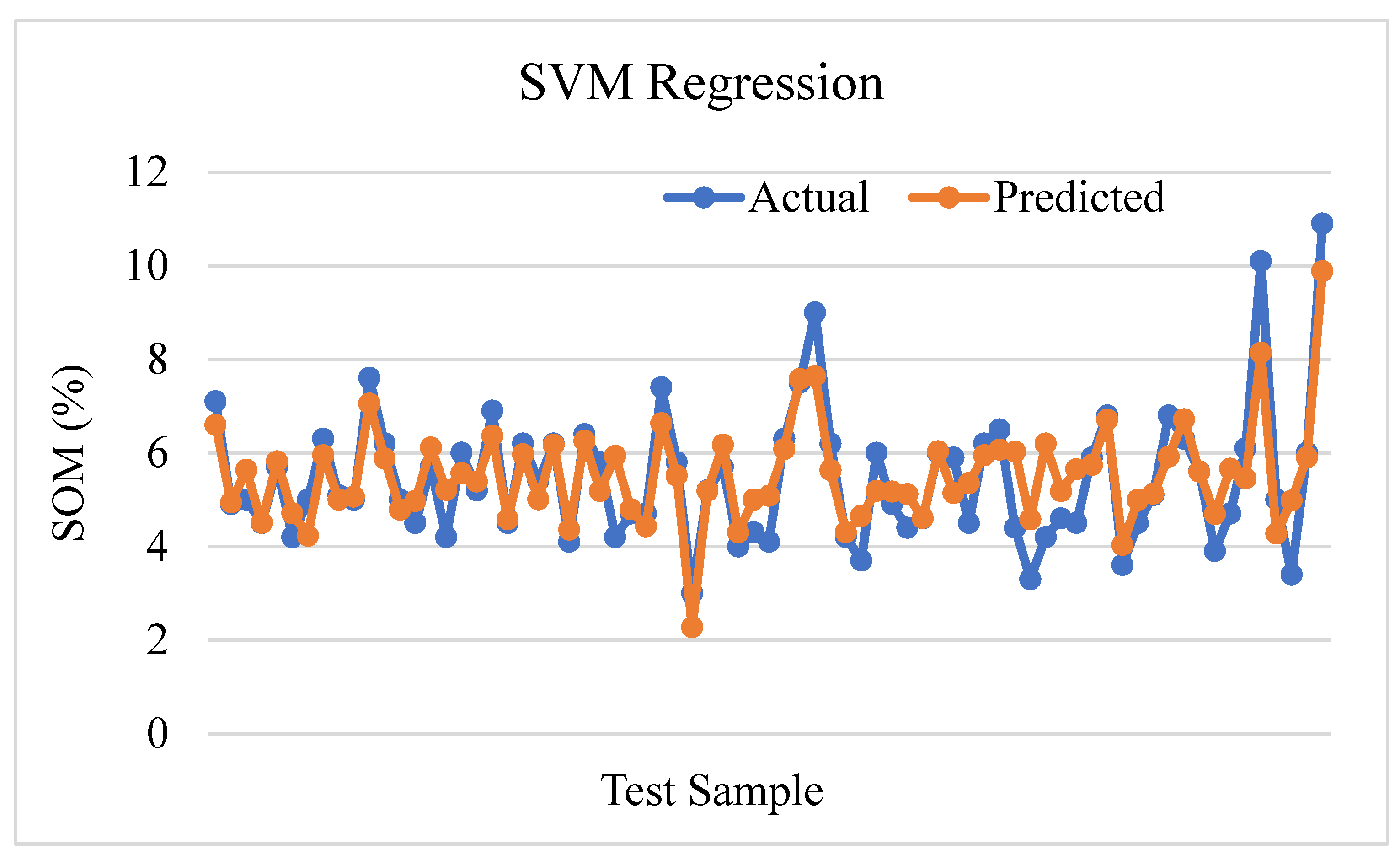
3.2.3. Machine Learning
4. Discussions
4.1. Effect of Sample Size and Data Variety on SOM Prediction
4.2. Comparisons of Performance in SOM Prediction
4.3. Limitations and Prospects
5. Conclusions
Author Contributions
Funding
Institutional Review Board Statement
Informed Consent Statement
Data Availability Statement
Conflicts of Interest
References
- Bauer, A.; Black, A.L. Black, Quantification of the effect of soil organic matter content on soil productivity. Soil Sci. Soc. Am. J. 1994, 58, 185–193. [Google Scholar]
- Gray, L.C.; Morant, P. Reconciling indigenous knowledge with scientific assessment of soil fertility changes in southwestern Burkina Faso. Geoderma 2003, 111, 425–437. [Google Scholar] [CrossRef]
- Lozano-García, B.; Parras-Alcántara, L.; De Albornoz, M.D.T.C. Effects of oil mill wastes on surface soil properties, runoff and soil losses in traditional olive groves in southern Spain. Catena 2011, 85, 187–193. [Google Scholar] [CrossRef]
- Anderson, W. Why Everyone Should Care about Mapping Soil Organic Matter and Carbon. Available online: https://swatmaps.com/2023/01/03/why-everyone-should-care-about-mapping-soil-organic-matter-and-carbon/ (accessed on 4 June 2023).
- Lal, R. Soil organic matter content and crop yield. J. Soil Water Conserv. 2020, 75, 27A–32A. [Google Scholar] [CrossRef]
- Schjønning, P.; Jensen, J.L.; Bruun, S.; Jensen, L.S.; Christensen, B.T.; Munkholm, L.J.; Oelofse, M.; Baby, S.; Knudsen, L. The role of soil organic matter for maintaining crop yields: Evidence for a renewed conceptual basis. Adv. Agron. 2018, 150, 35–79. [Google Scholar]
- Sprunger, C.D.; Martin, T.K. An integrated approach to assessing soil biological health. Adv. Agron. 2023, 182, 131. [Google Scholar]
- Bhattacharyya, S.S.; Ros, G.H.; Furtak, K.; Iqbal, H.M.; Parra-Saldívar, R. Soil carbon sequestration–An interplay between soil microbial community and soil organic matter dynamics. Sci. Total Environ. 2022, 815, 152928. [Google Scholar] [CrossRef]
- Schlesinger, W.H. Carbon sequestration in soils: Some cautions amidst optimism. Agric. Ecosyst. Environ. 2000, 82, 121–127. [Google Scholar] [CrossRef]
- Ding, J.; Zhang, Y.; Wang, M.; Sun, X.; Cong, J.; Deng, Y.; Lu, H.; Yuan, T.; Van Nostrand, J.D.; Li, D.; et al. Soil organic matter quantity and quality shape microbial community compositions of subtropical broadleaved forests. Mol. Ecol. 2015, 24, 5175–5185. [Google Scholar] [CrossRef]
- Tian, J.; He, N.; Hale, L.; Niu, S.; Yu, G.; Liu, Y.; Blagodatskaya, E.; Kuzyakov, Y.; Gao, Q.; Zhou, J. Soil organic matter availability and climate drive latitudinal patterns in bacterial diversity from tropical to cold temperate forests. Funct. Ecol. 2018, 32, 61–70. [Google Scholar] [CrossRef]
- Louis, B.P.; Maron, P.-A.; Viaud, V.; Leterme, P.; Menasseri-Aubry, S. Soil C and N models that integrate microbial diversity. Environ. Chem. Lett. 2016, 14, 331–344. Available online: https://www.ncbi.nlm.nih.gov/pmc/articles/PMC5011482/pdf/10311_2016_Article_571.pdf (accessed on 1 September 2021). [CrossRef]
- Kallenbach, C.M.; Frey, S.D.; Grandy, A.S. Direct evidence for microbial-derived soil organic matter formation and its ecophysiological controls. Nat. Commun. 2016, 7, 13630. [Google Scholar] [CrossRef]
- Cotrufo, M.F.; Lavallee, J.M. Soil organic matter formation, persistence, and functioning: A synthesis of current understanding to inform its conservation and regeneration. Adv. Agron. 2022, 172, 1–66. [Google Scholar]
- DVaughan; Malcolm, R. Soil Organic Matter and Biological Activity; Springer Science & Business Media: Berlin/Heidelberg, Germany, 2012. [Google Scholar]
- Esmaeilzadeh, J.; Ahangar, A.G. Influence of soil organic matter content on soil physical, chemical and biological properties. Int. J. Plant Anim. Environ. Sci. 2014, 4, 244–252. [Google Scholar]
- Ball, D.F. Loss-on-ignition as an estimate of organic matter and organic carbon in non-calcareous soils. J. Soil Sci. 1964, 15, 84–92. [Google Scholar] [CrossRef]
- Khaledian, Y.; Kiani, F.; Ebrahimi, S.; Brevik, E.C.; Aitkenhead-Peterson, J. Assessment and monitoring of soil degradation during land use change using multivariate analysis. Land Degrad. Dev. 2017, 28, 128–141. [Google Scholar] [CrossRef]
- García-Tomillo, A.; Mirás-Avalos, J.M.; Dafonte-Dafonte, J.; Paz-González, A. Estimating soil organic matter using interpolation methods with a electromagnetic induction sensor and topographic parameters: A case study in a humid region. Precis. Agric. 2017, 18, 882–897. [Google Scholar] [CrossRef]
- Kweon, G.; Lund, E.; Maxton, C. Soil organic matter and cation-exchange capacity sensing with on-the-go electrical conductivity and optical sensors. Geoderma 2013, 199, 80–89. [Google Scholar] [CrossRef]
- Kweon, G.; Maxton, C. Soil organic matter sensing with an on-the-go optical sensor. Biosyst. Eng. 2013, 115, 66–81. [Google Scholar] [CrossRef]
- Coelho, A.D.; Dias, B.G.; Assis, W.d.O.; Martins, F.d.A.; Pires, R.C. Monitoring of Soil Moisture and Atmospheric Sensors with Internet of Things (IoT) Applied in Precision Agriculture. In Proceedings of the 2020 XIV Technologies Applied to Electronics Teaching Conference (TAEE), Porto, Portugal, 8–10 July 2020; IEEE: Piscataway, NJ, USA; pp. 1–8. [Google Scholar]
- Thakur, D.; Kumar, Y.; Kumar, A.; Singh, P.K. Applicability of wireless sensor networks in precision agriculture: A review. Wirel. Pers. Commun. 2019, 107, 471–512. [Google Scholar] [CrossRef]
- Yinka-Banjo, C.; Ajayi, O. Sky-farmers: Applications of unmanned aerial vehicles (UAV) in agriculture. In Autonomous Vehicles; IntechOpen: London, UK, 2019; pp. 107–128. [Google Scholar]
- Ham, Y.; Han, K.K.; Lin, J.J.; Golparvar-Fard, M. Visual monitoring of civil infrastructure systems via camera-equipped Unmanned Aerial Vehicles (UAVs): A review of related works. Vis. Eng. 2016, 4, 1. [Google Scholar] [CrossRef]
- Yao, H.; Qin, R.; Chen, X. Unmanned aerial vehicle for remote sensing applications—A review. Remote Sens. 2019, 11, 1443. [Google Scholar] [CrossRef]
- McEvoy, J.F.; Hall, G.P.; McDonald, P.G. Evaluation of unmanned aerial vehicle shape, flight path and camera type for waterfowl surveys: Disturbance effects and species recognition. PeerJ 2016, 4, e1831. Available online: https://www.ncbi.nlm.nih.gov/pmc/articles/PMC4806640/pdf/peerj-04-1831.pdf (accessed on 1 September 2022). [CrossRef]
- Swain, K.C.; Thomson, S.J.; Jayasuriya, H.P.W. Adoption of an unmanned helicopter for low-altitude remote sensing to estimate yield and total biomass of a rice crop. Trans. ASABE 2010, 53, 21–27. [Google Scholar] [CrossRef]
- Stafford, J.V. Stafford, Implementing precision agriculture in the 21st century. J. Agric. Eng. Res. 2000, 76, 267–275. [Google Scholar] [CrossRef]
- Warren, G.; Metternicht, G. Agricultural applications of high-resolution digital multispectral imagery. Photogramm. Eng. Remote Sens. 2005, 71, 595–602. [Google Scholar] [CrossRef]
- Smith, G.D. The Guy Smith interviews: Rationale for Concepts in Soil Taxonomy (No. 11); Cornell University, Department of Agronomy: Ithaca, NY, USA, 1986. [Google Scholar]
- Stoner, E.R.; Baumgardner, M.F. Characteristic variations in reflectance of surface soils. Soil Sci. Soc. Am. J. 1981, 45, 1161–1165. [Google Scholar] [CrossRef]
- Sudduth, K.A.; Hummel, J.W. Evaluation of reflectance methods for soil organic matter sensing. Trans. ASAE 1991, 34, 1900–1909. [Google Scholar] [CrossRef]
- Sudduth, K.A.; Hummel, J.W. Geographic operating range evaluation of a NIR soil sensor. Trans. ASAE 1996, 39, 1599–1604. [Google Scholar] [CrossRef]
- Sullivan, D.G.; Shaw, J.N.; Rickman, D.; Mask, P.L.; Luvall, J.C. Using remote sensing data to evaluate surface soil properties in Alabama ultisols. Soil Sci. 2005, 170, 954–968. [Google Scholar] [CrossRef]
- Zarco-Tejada, P.J.; González-Dugo, V.; Berni, J.A.J. Fluorescence, temperature and narrow-band indices acquired from a UAV platform for water stress detection using a micro-hyperspectral imager and a thermal camera. Remote Sens. Environ. 2012, 117, 322–337. [Google Scholar] [CrossRef]
- Laliberte, A.S.; Rango, A.; Fredrickson, E.L. Multi-scale, object-oriented analysis of QuickBird imagery for determining percent cover in arid land vegetation. In Proceedings of the American Society for Photogrammetry and Remote Sensing Proceedings, Weslaco, TX, USA, 4–6 October 2005. [Google Scholar]
- Beeri, O.; Phillips, R.; Carson, P.; Liebig, M. Alternate satellite models for estimation of sugar beet residue nitrogen credit. Agric. Ecosyst. Environ. 2005, 107, 21–35. [Google Scholar] [CrossRef]
- Zhang, X.; Yan, G.; Li, Q.; Li, Z.; Wan, H.; Guo, Z. Evaluating the fraction of vegetation cover based on NDVI spatial scale correction model. Int. J. Remote Sens. 2006, 27, 5359–5372. [Google Scholar] [CrossRef]
- Shou, L.; Jia, L.; Cui, Z.; Chen, X.; Zhang, F. Using high-resolution satellite imaging to evaluate nitrogen status of winter wheat. J. Plant Nutr. 2007, 30, 1669–1680. [Google Scholar] [CrossRef]
- Bausch, W.C.; Khosla, R. QuickBird satellite versus ground-based multi-spectral data for estimating nitrogen status of irrigated maize. Precis. Agric. 2010, 11, 274–290. [Google Scholar] [CrossRef]
- Donoghue, D.N.M.; Watt, P.J. Using LiDAR to compare forest height estimates from IKONOS and Landsat ETM+ data in Sitka spruce plantation forests. J. Remote Sens. 2006, 27, 2161–2175. [Google Scholar] [CrossRef]
- Thenkabail, P.S.; Enclona, E.A.; Ashton, M.S.; Van Der Meer, B. Accuracy assessments of hyperspectral waveband performance for vegetation analysis applications. Remote Sens. Environ. 2004, 91, 354–376. [Google Scholar] [CrossRef]
- Gómez-Casero, M.T.; Castillejo-González, I.L.; García-Ferrer, A.; Peña-Barragán, J.M.; Jurado-Expósito, M.; García-Torres, L.; López-Granados, F. Spectral discrimination of wild oat and canary grass in wheat fields for less herbicide application. Agron. Sustain. Dev. 2010, 30, 689–699. [Google Scholar] [CrossRef]
- Peña-Barragán, J.M.; Ngugi, M.K.; Plant, R.E.; Six, J. Object-based crop identification using multiple vegetation indices, textural features and crop phenology. Remote Sens. Environ. 2011, 115, 1301–1316. [Google Scholar] [CrossRef]
- Castillejo-González, I.L.; López-Granados, F.; García-Ferrer, A.; Peña-Barragán, J.M.; Jurado-Expósito, M.; de la Orden, M.S.; González-Audicana, M. Object-and pixel-based analysis for mapping crops and their agro-environmental associated measures using QuickBird imagery. Comput. Electron. Agric. 2009, 68, 207–215. [Google Scholar] [CrossRef]
- Conforti, M.; Buttafuoco, G.; Leone, A.P.; Aucelli, P.P.; Robustelli, G.; Scarciglia, F. Studying the relationship between water-induced soil erosion and soil organic matter using Vis–NIR spectroscopy and geomorphological analysis: A case study in southern Italy. Catena 2013, 110, 44–58. [Google Scholar] [CrossRef]
- Stenberg, B.; Viscarra-Rossel, R.A.; Mouazen, A.M.; Wetterlind, J. Visible and near infrared spectroscopy in soil science. Adv. Agron. 2010, 107, 163–215. [Google Scholar]
- McBratney, A.B.; Minasny, B.; Rossel, R.V. Spectral soil analysis and inference systems: A powerful combination for solving the soil data crisis. Geoderma 2006, 136, 272–278. [Google Scholar] [CrossRef]
- Viscarra Rossel, R.A.; Walvoort, D.J.J.; McBratney, A.B.; Janik, L.J.; Skjemstad, J.O. Visible, near infrared, mid infrared or combined diffuse reflectance spectroscopy for simultaneous assessment of various soil properties. Geoderma 2006, 131, 59–75. [Google Scholar] [CrossRef]
- Stenberg, B. Effects of soil sample pretreatments and standardised rewetting as interacted with sand classes on Vis-NIR predictions of clay and soil organic carbon. Geoderma 2010, 158, 15–22. [Google Scholar] [CrossRef]
- Conforti, M.; Castrignanò, A.; Robustelli, G.; Scarciglia, F.; Stelluti, M.; Buttafuoco, G. Laboratory-based Vis–NIR spectroscopy and partial least square regression with spatially correlated errors for predicting spatial variation of soil organic matter content. Catena 2015, 124, 60–67. [Google Scholar] [CrossRef]
- Ba, Y.; Liu, J.; Han, J.; Zhang, X. Application of Vis-NIR spectroscopy for determination the content of organic matter in saline-alkali soils. Spectrochim. Acta Part A Mol. Biomol. Spectrosc. 2020, 229, 117863. [Google Scholar] [CrossRef] [PubMed]
- Xu, Z.; Zhao, X.; Guo, X.; Guo, J. Deep learning application for predicting soil organic matter content by VIS-NIR spectroscopy. Comput. Intell. Neurosci. 2019, 2019, 3563761. [Google Scholar] [CrossRef]
- Hummel, J.; Sudduth, K.; Hollinger, S. Soil moisture and organic matter prediction of surface and subsurface soils using an NIR soil sensor. Comput. Electron. Agric. 2001, 32, 149–165. [Google Scholar] [CrossRef]
- Stiglitz, R.Y.; Mikhailova, E.A.; Sharp, J.L.; Post, C.J.; Schlautman, M.A.; Gerard, P.D.; Cope, M.P. Predicting soil organic carbon and total nitrogen at the farm scale using quantitative color sensor measurements. Agronomy 2018, 8, 212. [Google Scholar] [CrossRef]
- Ge, X.; Wang, J.; Ding, J.; Cao, X.; Zhang, Z.; Liu, J.; Li, X. Combining UAV-based hyperspectral imagery and machine learning algorithms for soil moisture content monitoring. PeerJ 2019, 7, e6926. [Google Scholar] [CrossRef]
- Zheng, J.; Yuan, S.; Wu, W.; Li, W.; Yu, L.; Fu, H.; Coomes, D. Surveying coconut trees using high-resolution satellite imagery in remote atolls of the Pacific Ocean. Remote Sens. Environ. 2023, 287, 113485. [Google Scholar] [CrossRef]
- Eskandari, R.; Mahdianpari, M.; Mohammadimanesh, F.; Salehi, B.; Brisco, B.; Homayouni, S. Meta-analysis of unmanned aerial vehicle (UAV) imagery for agro-environmental monitoring using machine learning and statistical models. Remote Sens. 2020, 12, 3511. [Google Scholar] [CrossRef]
- Jay, S.; Baret, F.; Dutartre, D.; Malatesta, G.; Héno, S.; Comar, A.; Weiss, M.; Maupas, F. Exploiting the centimeter resolution of UAV multispectral imagery to improve remote-sensing estimates of canopy structure and biochemistry in sugar beet crops. Remote Sens. Environ. 2019, 231, 110898. [Google Scholar] [CrossRef]
- Heil, J.; Jörges, C.; Stumpe, B. Fine-Scale Mapping of Soil Organic Matter in Agricultural Soils Using UAVs and Machine Learning. Remote Sens. 2022, 14, 3349. [Google Scholar] [CrossRef]
- Partel, V.; Costa, L.; Ampatzidis, Y. Smart tree crop sprayer utilizing sensor fusion and artificial intelligence. Comput. Electron. Agric. 2021, 191, 106556. [Google Scholar] [CrossRef]
- Sothe, C.; Gonsamo, A.; Arabian, J.; Snider, J. Large scale mapping of soil organic carbon concentration with 3D machine learning and satellite observations. Geoderma 2022, 405, 115402. [Google Scholar] [CrossRef]
- Conant, R.T.; Ryan, M.G.; Ågren, G.I.; Birge, H.E.; Davidson, E.A.; Eliasson, P.E.; Evans, S.E.; Frey, S.D.; Giardina, C.P.; Hopkins, F.M.; et al. Temperature and soil organic matter decomposition rates–synthesis of current knowledge and a way forward. Glob. Chang. Biol. 2011, 17, 3392–3404. [Google Scholar] [CrossRef]
- Kirschbaum, M.U. The temperature dependence of soil organic matter decomposition, and the effect of global warming on soil organic C storage. Soil Biol. Biochem. 1995, 27, 753–760. [Google Scholar] [CrossRef]
- Ren, Q.; Yuan, J.; Wang, J.; Liu, X.; Ma, S.; Zhou, L.; Miao, L.; Zhang, J. Water level has higher influence on soil organic carbon and microbial community in Poyang Lake wetland than vegetation type. Microorganisms 2022, 10, 131. Available online: https://mdpi-res.com/d_attachment/microorganisms/microorganisms-10-00131/article_deploy/microorganisms-10-00131-v2.pdf?version=1641793176 (accessed on 12 February 2023). [CrossRef]
- Wibowo, H.; Kasno, A. Soil organic carbon and total nitrogen dynamics in paddy soils on the Java Island, Indonesia. IOP Conf. Ser. Earth Environ. Sci. 2021, 648, 012192. [Google Scholar] [CrossRef]
- Kang, J.; Hesterberg, D.; Osmond, D.L. Soil organic matter effects on phosphorus sorption: A path analysis. Soil Sci. Soc. Am. J. 2009, 73, 360–366. [Google Scholar] [CrossRef]
- Wang, F.L.; Huang, P.M. Effects of organic matter on the rate of potassium adsorption by soils. Can. J. Soil Sci. 2001, 81, 325–330. [Google Scholar] [CrossRef]
- Zhou, W.; Han, G.; Liu, M.; Li, X. Effects of soil pH and texture on soil carbon and nitrogen in soil profiles under different land uses in Mun River Basin, Northeast Thailand. PeerJ 2019, 7, e7880. Available online: https://www.ncbi.nlm.nih.gov/pmc/articles/PMC6798867/pdf/peerj-07-7880.pdf (accessed on 23 October 2022). [CrossRef]
- Zhang, Y.; Guo, L.; Chen, Y.; Shi, T.; Luo, M.; Ju, Q.; Zhang, H.; Wang, S. Prediction of soil organic carbon based on Landsat 8 monthly NDVI data for the Jianghan Plain in Hubei Province, China. Remote Sens. 2019, 11, 1683. [Google Scholar] [CrossRef]
- Hong, S.; Gan, P.; Chen, A. Environmental controls on soil pH in planted forest and its response to nitrogen deposition. Environ. Res. 2019, 172, 159–165. [Google Scholar] [CrossRef]
- Qu, W.; Han, G.; Wang, J.; Li, J.; Zhao, M.; He, W.; Li, X.; Wei, S. Short-term effects of soil moisture on soil organic carbon decomposition in a coastal wetland of the Yellow River Delta. Hydrobiologia 2021, 848, 3259–3271. [Google Scholar] [CrossRef]
- Kerr, D.D.; Ochsner, T.E. Soil organic carbon more strongly related to soil moisture than soil temperature in temperate grasslands. Soil Sci. Soc. Am. J. 2020, 84, 587–596. [Google Scholar] [CrossRef]
- Junting, Y.; Xiaosong, L.; Bo, W.; Junjun, W.; Bin, S.; Changzhen, Y.; Zhihai, G. High spatial resolution topsoil organic matter content mapping across desertified land in northern China. Front. Environ. Sci. 2021, 9, 668912. [Google Scholar] [CrossRef]
- Keen, Y.C.; Jalloh, M.B.; Ahmed, O.H.; Sudin, M.; Besar, N.A. Soil organic matter and related soil properties in forest, grassland and cultivated land use types. Int. J. Phys. Sci. 2011, 6, 7410–7415. [Google Scholar]


| Soil Parameters | Mean | SD | Minimum | Median | Maximum |
|---|---|---|---|---|---|
| Temperature (°C) | 22.81 | 6.13 | 8.30 | 23.40 | 34.50 |
| Humidity (%RH) | 26.37 | 12.20 | 5.60 | 23.80 | 72.70 |
| Soil pH | 7.63 | 0.92 | 3.00 | 8.03 | 9.00 |
| Nitrogen (mg/kg) | 34.99 | 15.21 | 4.00 | 29.00 | 94.00 |
| Phosphorous (mg/kg) | 49.35 | 19.70 | 5.00 | 42.50 | 135.00 |
| Potassium (mg/kg) | 107.14 | 42.86 | 13.00 | 93.50 | 285.00 |
| NDVI | 0.41 | 0.16 | 0.21 | 0.42 | 0.75 |
| Total N (%) | 0.29 | 0.10 | 0.14 | 0.27 | 0.88 |
| H2O Total Organic C, ppm | 248.71 | 66.54 | 91.90 | 241.35 | 474.90 |
| H2O Total N, ppm | 37.00 | 18.73 | 11.90 | 32.15 | 197.40 |
| H2O Nitrate, ppm NO3-N | 17.46 | 14.28 | 1.20 | 14.90 | 167.00 |
| H2O Ammonium, ppm NH4-N | 1.81 | 0.50 | 0.96 | 1.75 | 4.08 |
| H2O Inorganic Nitrogen, ppm N | 19.27 | 14.34 | 3.10 | 16.60 | 170.40 |
| H2O Organic N, ppm N | 17.75 | 7.09 | 4.30 | 16.50 | 43.90 |
| Soil Organic Matter, %LOI | 5.5622 | 1.748 | 2.9 | 5.3 | 19.6 |
| Term | Coef | SE Coef | T-Value | p-Value | VIF |
|---|---|---|---|---|---|
| Constant | 0.254 | 0.507 | 0.50 | 0.616 | |
| Temperature (°C) | 0.0471 | 0.0108 | 4.38 | 0.000 | 2.38 |
| Humidity (%RH) | −0.00296 | 0.00453 | −0.65 | 0.514 | 1.67 |
| Soil pH | −0.0818 | 0.0502 | −1.63 | 0.104 | 1.16 |
| Nitrogen (mg/kg) | 0.0771 | 0.0144 | 5.36 | 0.000 | 26.25 |
| Phosphorous (mg/kg) | −0.0749 | 0.0128 | −5.83 | 0.000 | 35.10 |
| Potassium (mg/kg) | 0.01457 | 0.00264 | 5.53 | 0.000 | 6.99 |
| NDVI | −0.926 | 0.339 | −2.74 | 0.006 | 1.58 |
| Total N, % | 16.387 | 0.703 | 23.31 | 0.000 | 2.49 |
| H2O Total Organic C, ppm | 0.00953 | 0.00169 | 5.65 | 0.000 | 6.91 |
| H2O Total N, ppm | −0.01508 | 0.00375 | −4.02 | 0.000 | 2.70 |
| H2O Organic N, ppm N | −0.1025 | 0.0192 | −5.33 | 0.000 | 10.18 |
| S | R-sq | R-sq (adj) | R-sq (pred) |
|---|---|---|---|
| 0.853289 | 76.82% | 76.17% | 74.58% |
| Source | DF | Adj SS | Adj MS | F-Value | p-Value |
|---|---|---|---|---|---|
| Regression | 11 | 936.36 | 85.123 | 116.91 | 0.000 |
| Temperature (°C) | 1 | 13.95 | 13.952 | 19.16 | 0.000 |
| Humidity (%RH) | 1 | 0.31 | 0.311 | 0.43 | 0.514 |
| Soil pH | 1 | 1.93 | 1.934 | 2.66 | 0.104 |
| Nitrogen (mg/kg) | 1 | 20.91 | 20.907 | 28.71 | 0.000 |
| Phosphorous (mg/kg) | 1 | 24.73 | 24.726 | 33.96 | 0.000 |
| Potassium (mg/kg) | 1 | 22.27 | 22.272 | 30.59 | 0.000 |
| NDVI | 1 | 5.45 | 5.454 | 7.49 | 0.006 |
| Total N, % | 1 | 395.58 | 395.579 | 543.30 | 0.000 |
| H2O Total Organic C, ppm | 1 | 23.21 | 23.214 | 31.88 | 0.000 |
| H2O Total N, ppm | 1 | 11.79 | 11.791 | 16.19 | 0.000 |
| H2O Organic N, ppm N | 1 | 20.71 | 20.712 | 28.45 | 0.000 |
| Error | 388 | 282.50 | 0.728 | ||
| Total | 399 | 1218.86 |
| Obs | Soil Organic Matter, %LOI | Fit | Residuals | Std Residuals | ||
|---|---|---|---|---|---|---|
| 38 | 5.700 | 5.755 | −0.055 | −0.07 | X * | |
| 59 | 4.500 | 4.061 | 0.439 | 0.54 | X | |
| 108 | 6.900 | 4.890 | 2.010 | 2.38 | R * | |
| 110 | 6.200 | 6.583 | −0.383 | −0.48 | X | |
| 118 | 6.600 | 4.816 | 1.784 | 2.14 | R | |
| 126 | 5.800 | 3.592 | 2.208 | 2.66 | R | |
| 130 | 5.600 | 3.557 | 2.043 | 2.45 | R | |
| 210 | 12.400 | 9.771 | 2.629 | 3.13 | R | |
| 211 | 10.600 | 8.470 | 2.130 | 2.54 | R | |
| 212 | 19.600 | 14.491 | 5.109 | 6.36 | R | X |
| 213 | 10.100 | 7.829 | 2.271 | 2.69 | R | |
| 247 | 7.700 | 4.587 | 3.113 | 3.74 | R | |
| 249 | 5.600 | 5.270 | 0.330 | 0.41 | X | |
| 256 | 6.900 | 3.636 | 3.264 | 3.91 | R | |
| 328 | 3.000 | 1.337 | 1.663 | 2.47 | R | X |
| Model | R-Square | Mean Square Error | Root Mean Square Error | Mean Absolute Error |
|---|---|---|---|---|
| Linear Regression | 0.7499 | 0.4997 | 0.7069 | 0.5872 |
| Elastic Net Regression | 0.5387 | 0.9215 | 0.9599 | 0.7398 |
| Lasso Regression | 0.5264 | 0.9462 | 0.9727 | 0.7423 |
| Ridge Regression | 0.7304 | 0.5386 | 0.7339 | 0.5949 |
| Random Forest | 0.8464 | 0.3068 | 0.5539 | 0.4280 |
| SGD Regression | 0.7301 | 0.5392 | 0.7343 | 0.6198 |
| SVM Regression | 0.7400 | 0.5193 | 0.7206 | 0.5430 |
Disclaimer/Publisher’s Note: The statements, opinions and data contained in all publications are solely those of the individual author(s) and contributor(s) and not of MDPI and/or the editor(s). MDPI and/or the editor(s) disclaim responsibility for any injury to people or property resulting from any ideas, methods, instructions or products referred to in the content. |
© 2024 by the authors. Licensee MDPI, Basel, Switzerland. This article is an open access article distributed under the terms and conditions of the Creative Commons Attribution (CC BY) license (https://creativecommons.org/licenses/by/4.0/).
Share and Cite
Uddin, M.J.; Sherrell, J.; Emami, A.; Khaleghian, M. Application of Artificial Intelligence and Sensor Fusion for Soil Organic Matter Prediction. Sensors 2024, 24, 2357. https://doi.org/10.3390/s24072357
Uddin MJ, Sherrell J, Emami A, Khaleghian M. Application of Artificial Intelligence and Sensor Fusion for Soil Organic Matter Prediction. Sensors. 2024; 24(7):2357. https://doi.org/10.3390/s24072357
Chicago/Turabian StyleUddin, Md Jasim, Jordan Sherrell, Anahita Emami, and Meysam Khaleghian. 2024. "Application of Artificial Intelligence and Sensor Fusion for Soil Organic Matter Prediction" Sensors 24, no. 7: 2357. https://doi.org/10.3390/s24072357
APA StyleUddin, M. J., Sherrell, J., Emami, A., & Khaleghian, M. (2024). Application of Artificial Intelligence and Sensor Fusion for Soil Organic Matter Prediction. Sensors, 24(7), 2357. https://doi.org/10.3390/s24072357