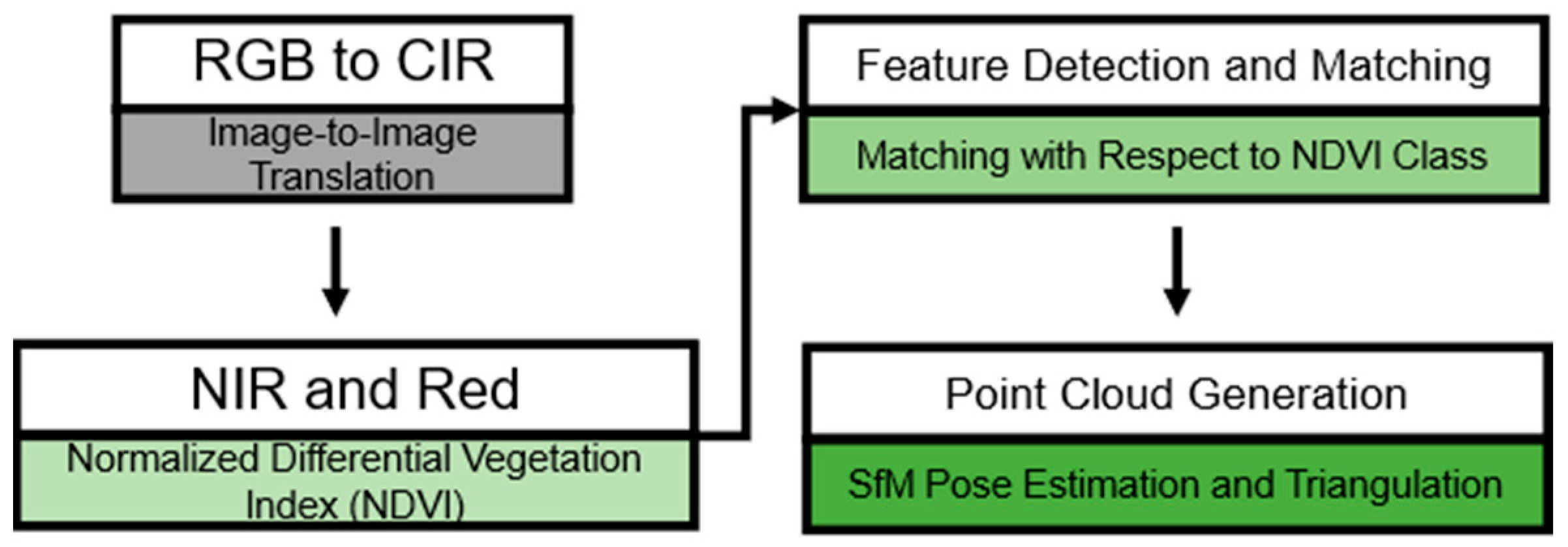
Figure 1.
Two-stage framework separated into the machine learning technique (gray) and the application in three steps (green). Firstly (gray), the CIR image is generated from RGB with image-to-image translation. Then (light green), the NDVI is calculated with the generated NIR and red band. Afterwards, (medium green), the NDVI segmentation and classification is used to match the detected features accordingly. Finally (dark green), pose estimation and triangulation are used to generate a sparse 3D point cloud.
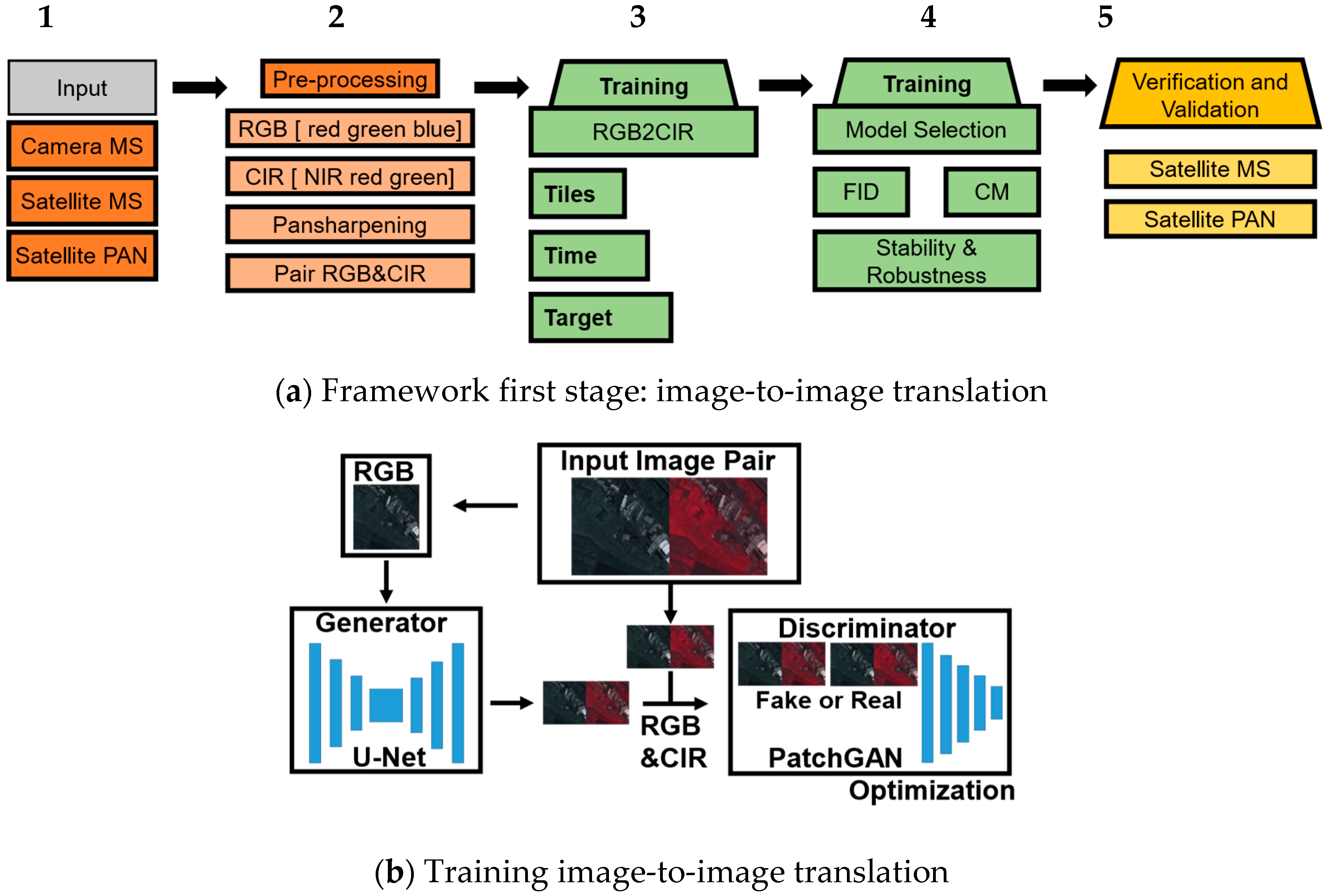
Figure 2.
First stage of the two-stage workflow. (a) Image-to-image translation in 5 steps for RGB2CIR simulation. In general, input and pre-processing (orange), training and testing (green) and verification and validation (yellow) (b) Image-to-image translation training.
Figure 2.
First stage of the two-stage workflow. (a) Image-to-image translation in 5 steps for RGB2CIR simulation. In general, input and pre-processing (orange), training and testing (green) and verification and validation (yellow) (b) Image-to-image translation training.
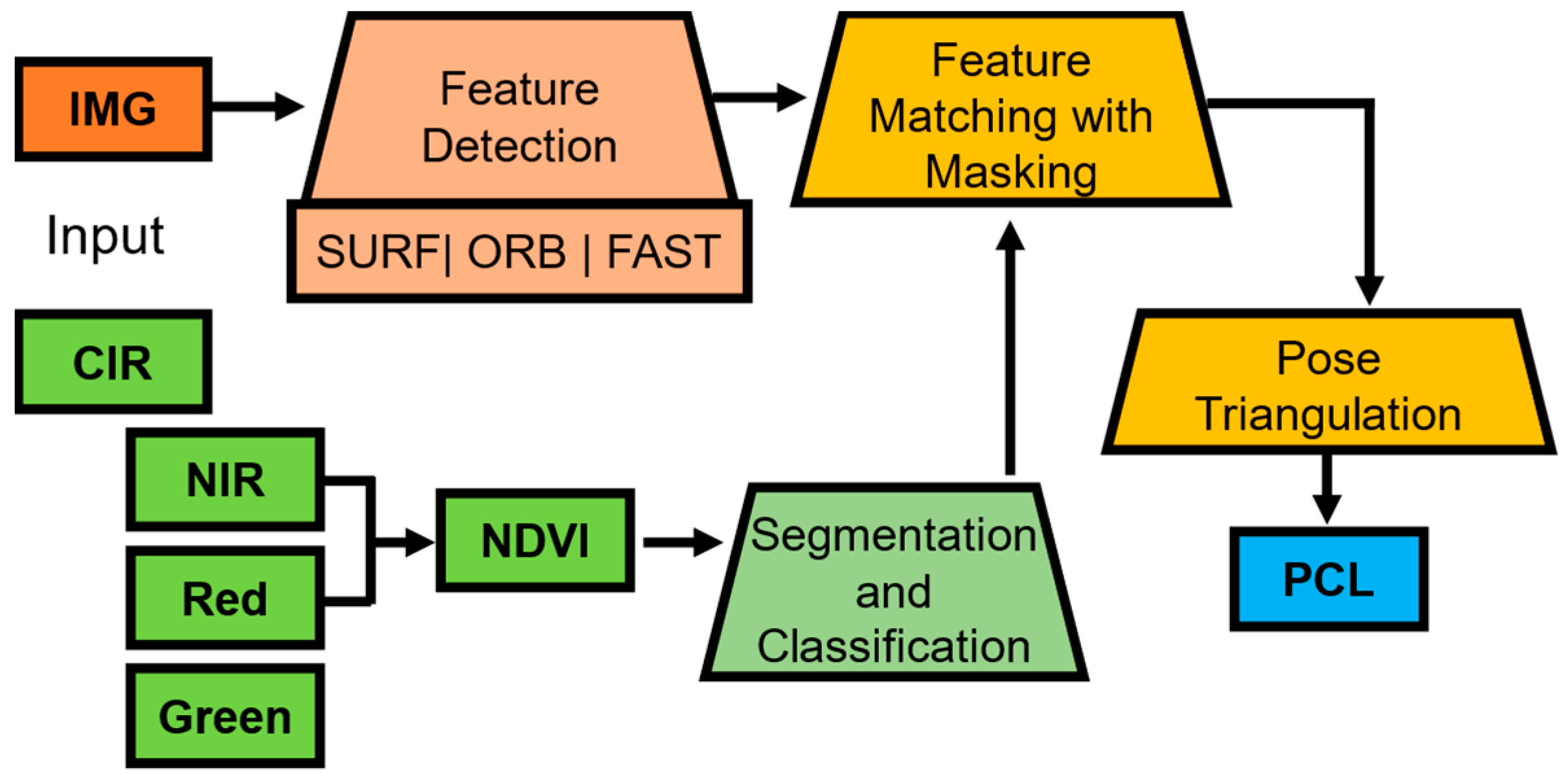
Figure 3.
Framework second stage: segmentation-driven two-view SfM algorithm. The processing steps are grouped by color, the NDVI related processing (green), the input, feature detection (orange), feature processing (yellow) and the output (blue).
Figure 3.
Framework second stage: segmentation-driven two-view SfM algorithm. The processing steps are grouped by color, the NDVI related processing (green), the input, feature detection (orange), feature processing (yellow) and the output (blue).
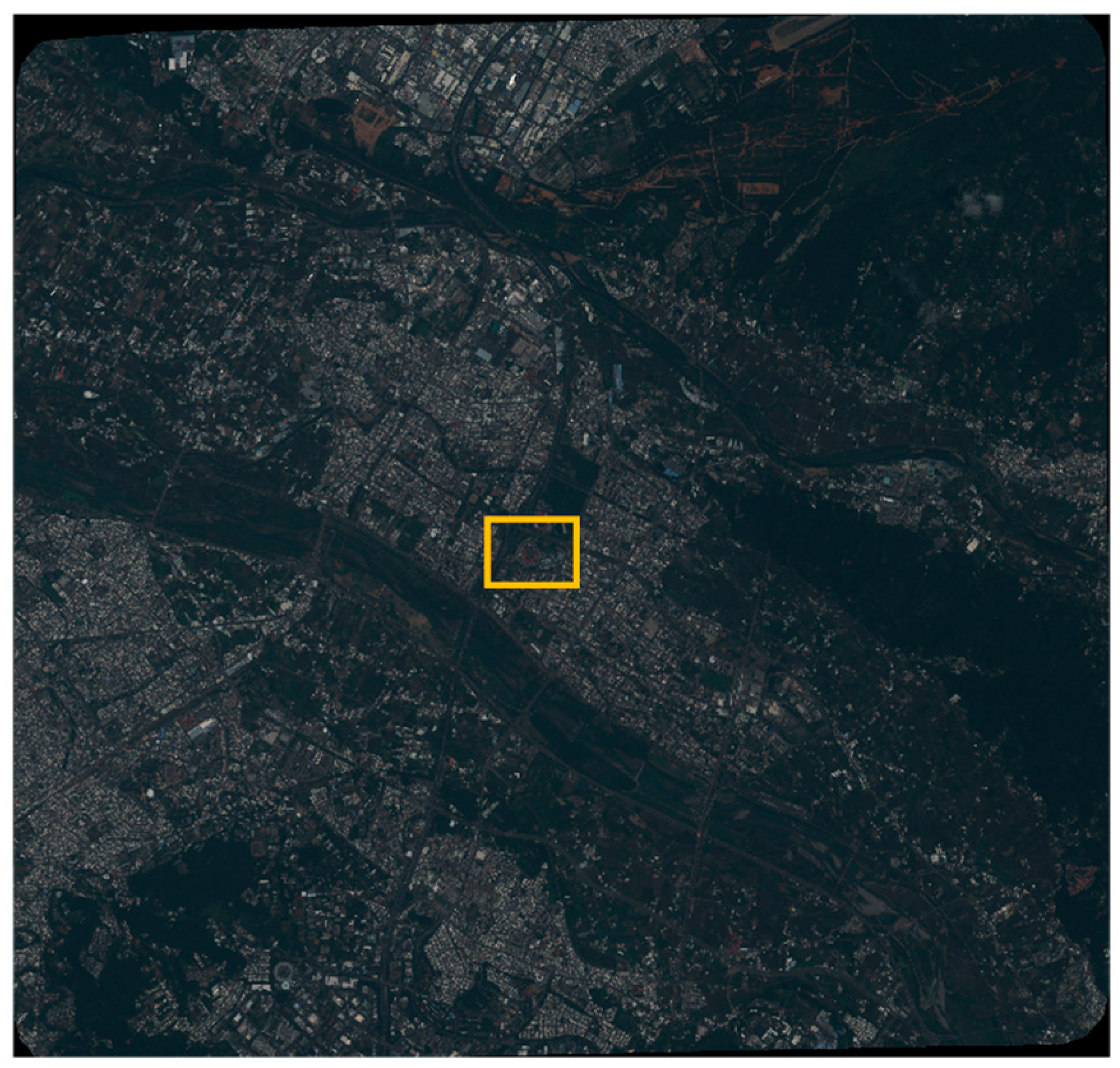
Figure 4.
Pleiades VHR satellite imagery, with the nadir view in true color (RGB). The location of the study target is marked in orange and used for validation (see
Section 3.2.3).
Figure 4.
Pleiades VHR satellite imagery, with the nadir view in true color (RGB). The location of the study target is marked in orange and used for validation (see
Section 3.2.3).
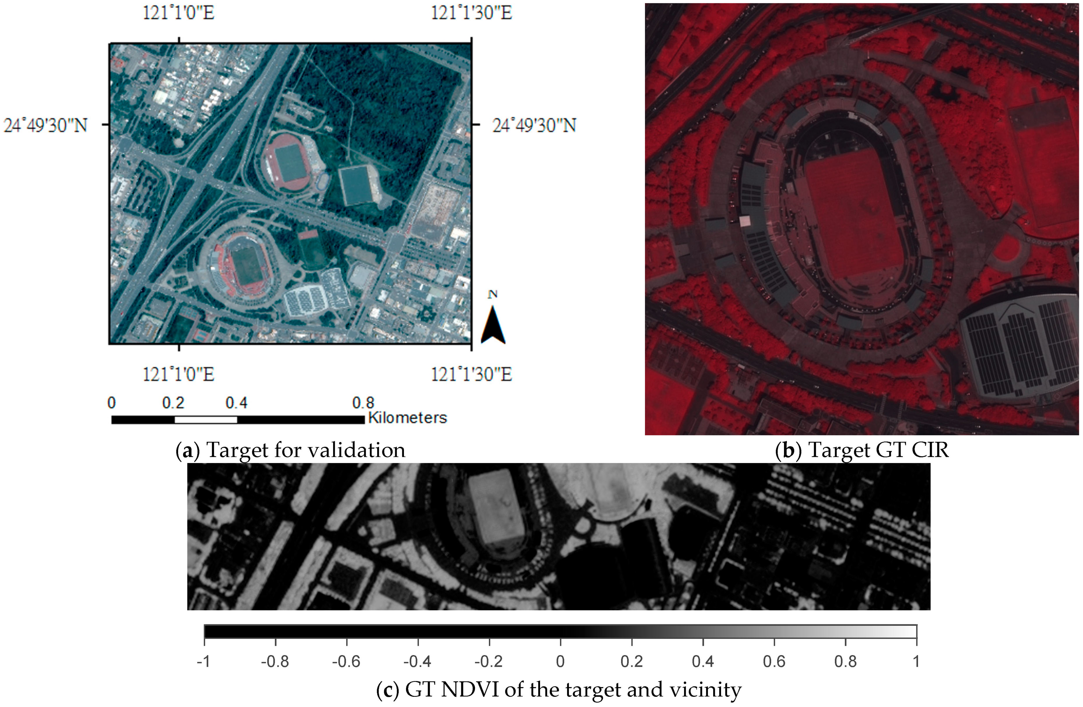
Figure 5.
The target for validation captured by Pleiades VHR satellite. (
a) The target stadium; (
b) the geolocation of the target (marked in orange in
Figure 4); (
c) the target ground truth (GT) CIR image. GT NDVI of the target building and its vicinity.
Figure 5.
The target for validation captured by Pleiades VHR satellite. (
a) The target stadium; (
b) the geolocation of the target (marked in orange in
Figure 4); (
c) the target ground truth (GT) CIR image. GT NDVI of the target building and its vicinity.
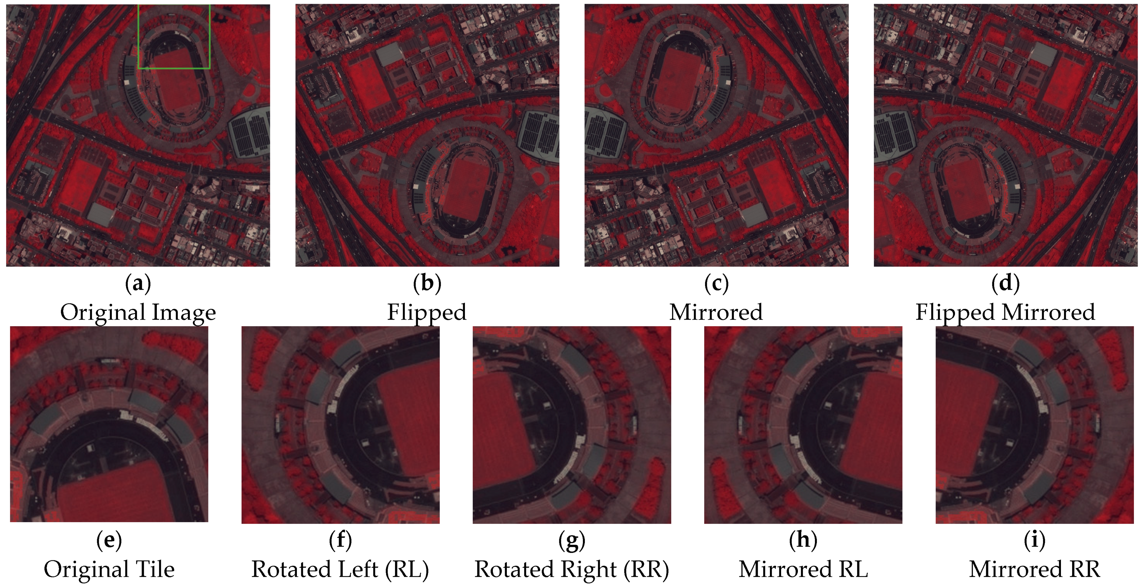
Figure 6.
Morphological changes on the image covering the target and image tiles. (a) Original cropped CIR image of Pleiades Satellite Imagery (1024 × 1024 × 3). A single tile, the white rectangle in (a), is shown as (e). (b–d) and (f–i) are the morphed images of (a) and (e), respectively.
Figure 6.
Morphological changes on the image covering the target and image tiles. (a) Original cropped CIR image of Pleiades Satellite Imagery (1024 × 1024 × 3). A single tile, the white rectangle in (a), is shown as (e). (b–d) and (f–i) are the morphed images of (a) and (e), respectively.
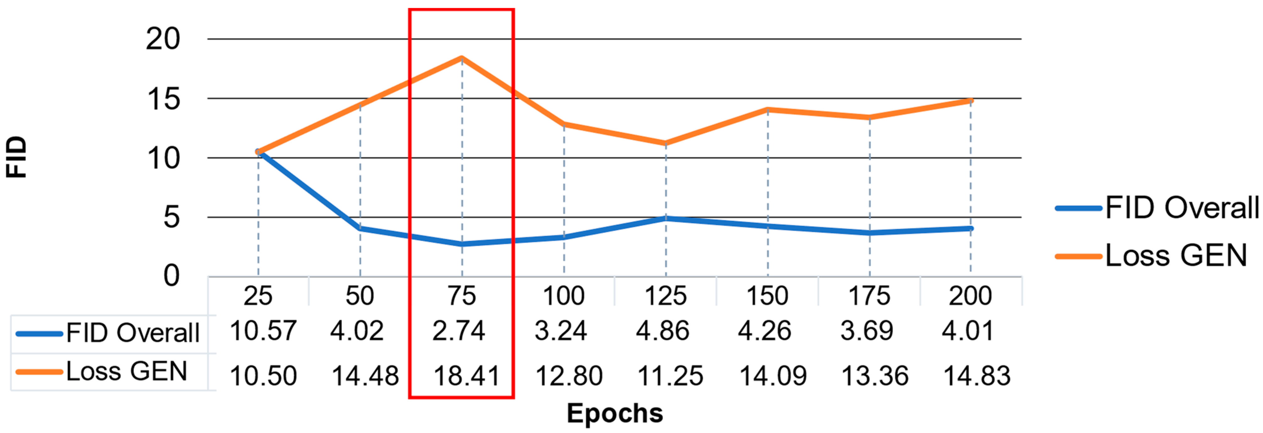
Figure 7.
Training over 200 epochs for model selection. The generator loss (loss GEN) plotted in orange and, in contrast, FID calculation results in blue.
Figure 7.
Training over 200 epochs for model selection. The generator loss (loss GEN) plotted in orange and, in contrast, FID calculation results in blue.
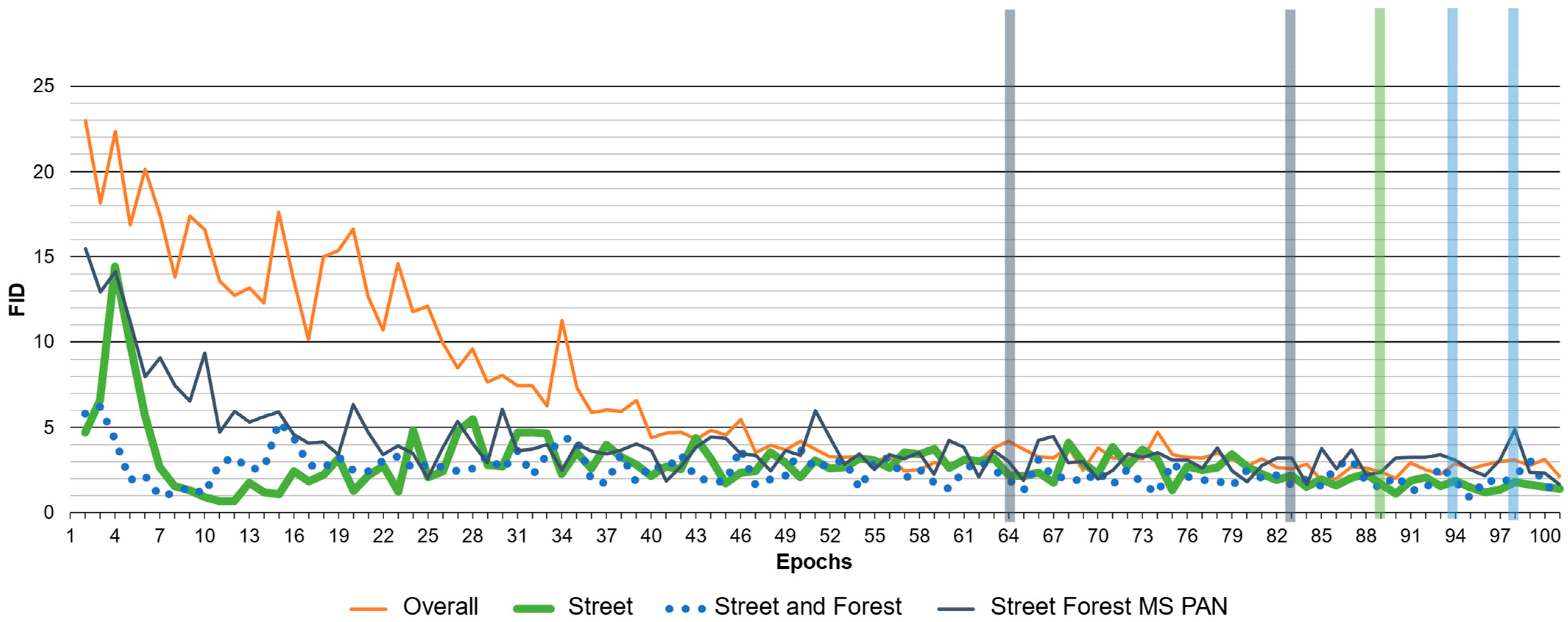
Figure 8.
Training Pix2Pix for model selection with FID. The epochs with the best FID and CM are marked for every test run, expect overall, with colored bars respectivly. The numbers are summarized in
Table 5.
Figure 8.
Training Pix2Pix for model selection with FID. The epochs with the best FID and CM are marked for every test run, expect overall, with colored bars respectivly. The numbers are summarized in
Table 5.
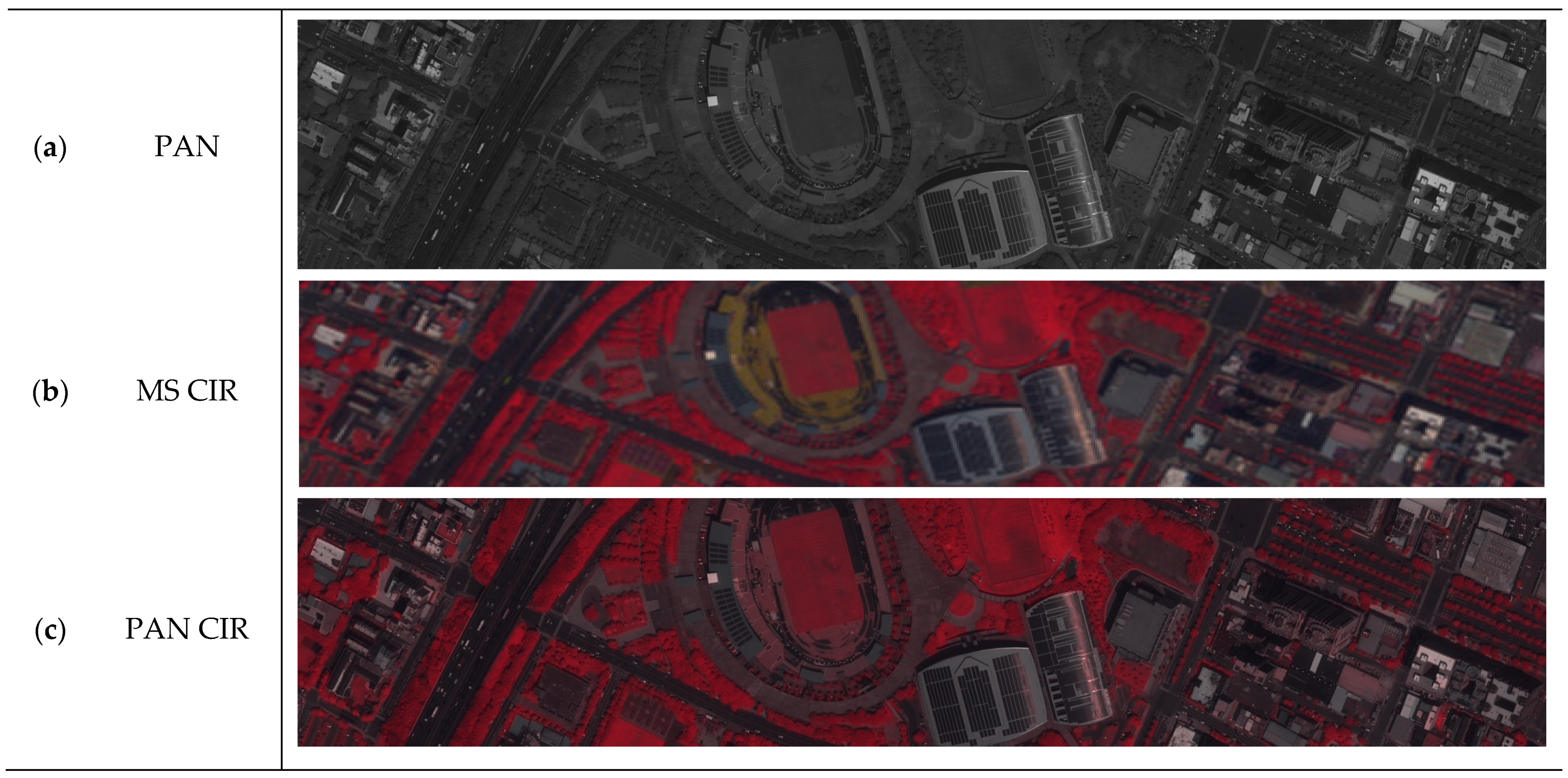
Figure 9.
CIR pansharpening on the target. The high-resolution panchromatic image is used to increase the resolution of the composite CIR image while preserving spectral information. From top to bottom, (a) panchromatic, (b) color infrared created from multi-spectral bands, and (c) pansharpened color infrared are shown.
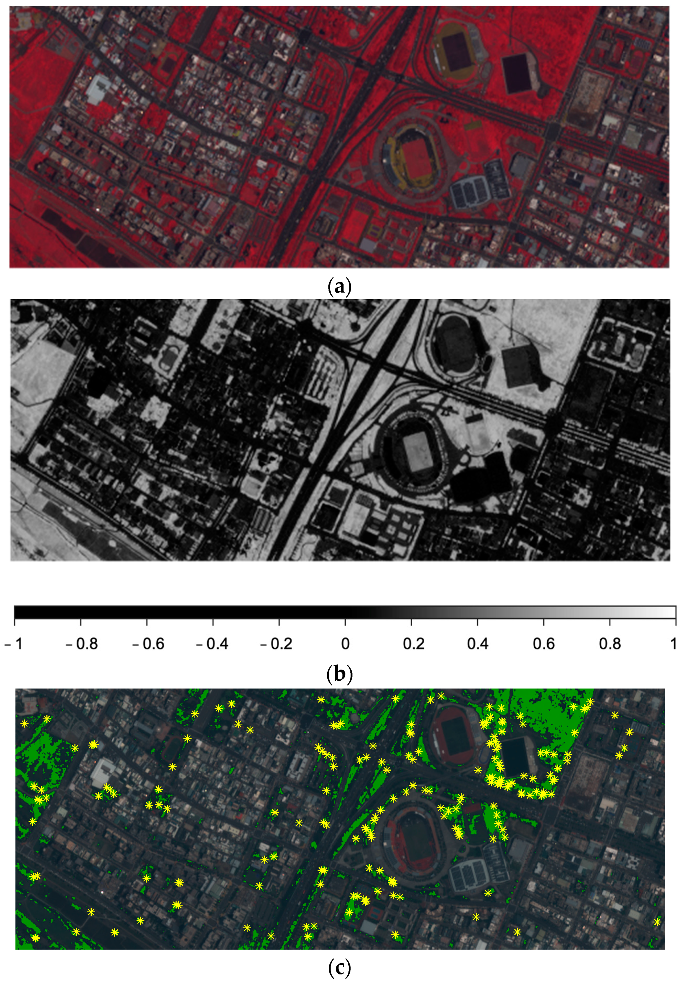
Figure 10.
Example of vegetation feature removal to the north of the stadium. (a) CIR images; (b) NDVI image with legend; (c) identified SURF features (yellos asterisks) within dense vegetated areas (green) using 0.6 as the threshold.
Figure 10.
Example of vegetation feature removal to the north of the stadium. (a) CIR images; (b) NDVI image with legend; (c) identified SURF features (yellos asterisks) within dense vegetated areas (green) using 0.6 as the threshold.
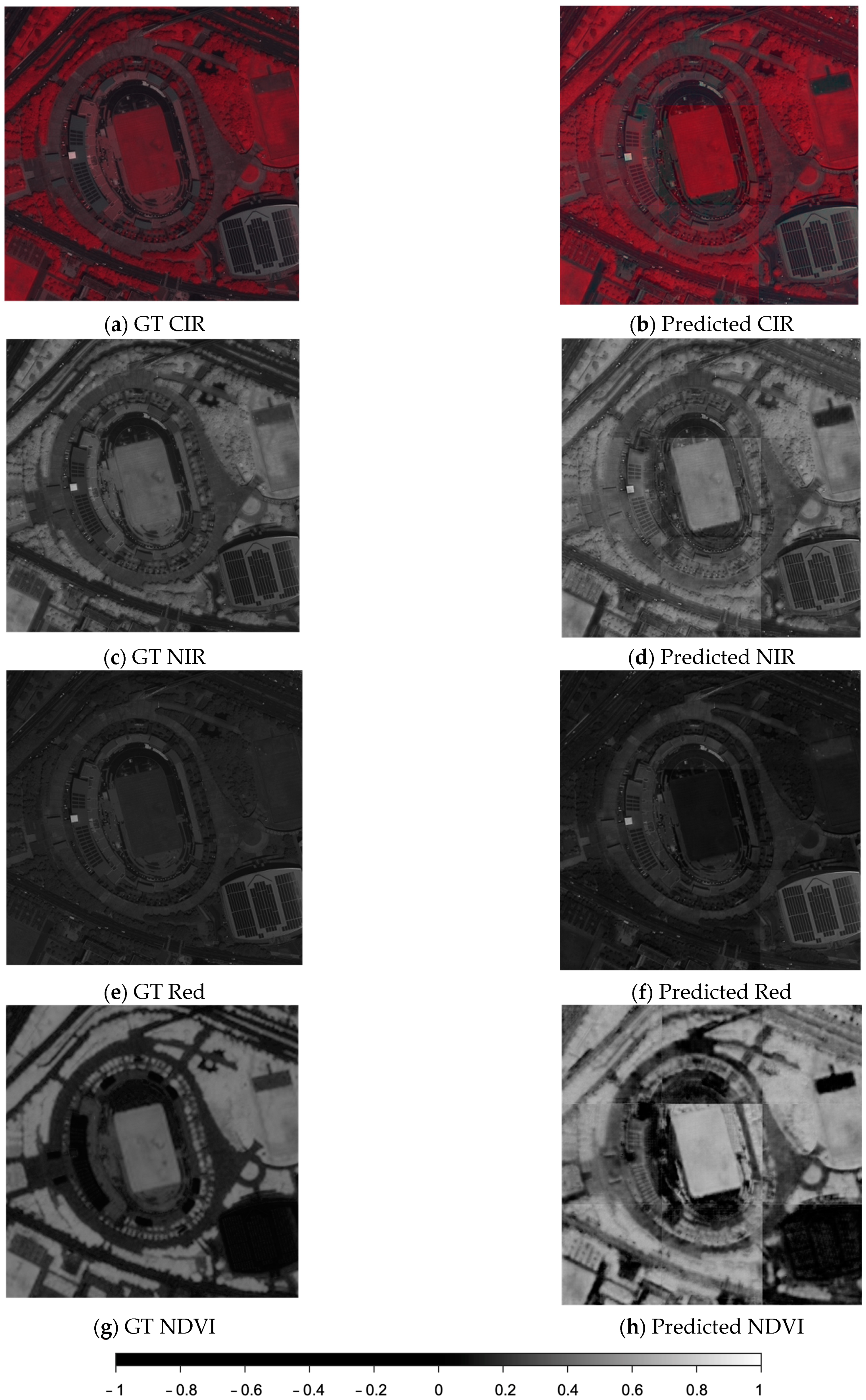
Figure 11.
Comparison between the prediction and the ground truth (GT) of the CIR, NIR and NDVI (incl. legend) of the main target (a stadium) and vicinity.
Figure 11.
Comparison between the prediction and the ground truth (GT) of the CIR, NIR and NDVI (incl. legend) of the main target (a stadium) and vicinity.
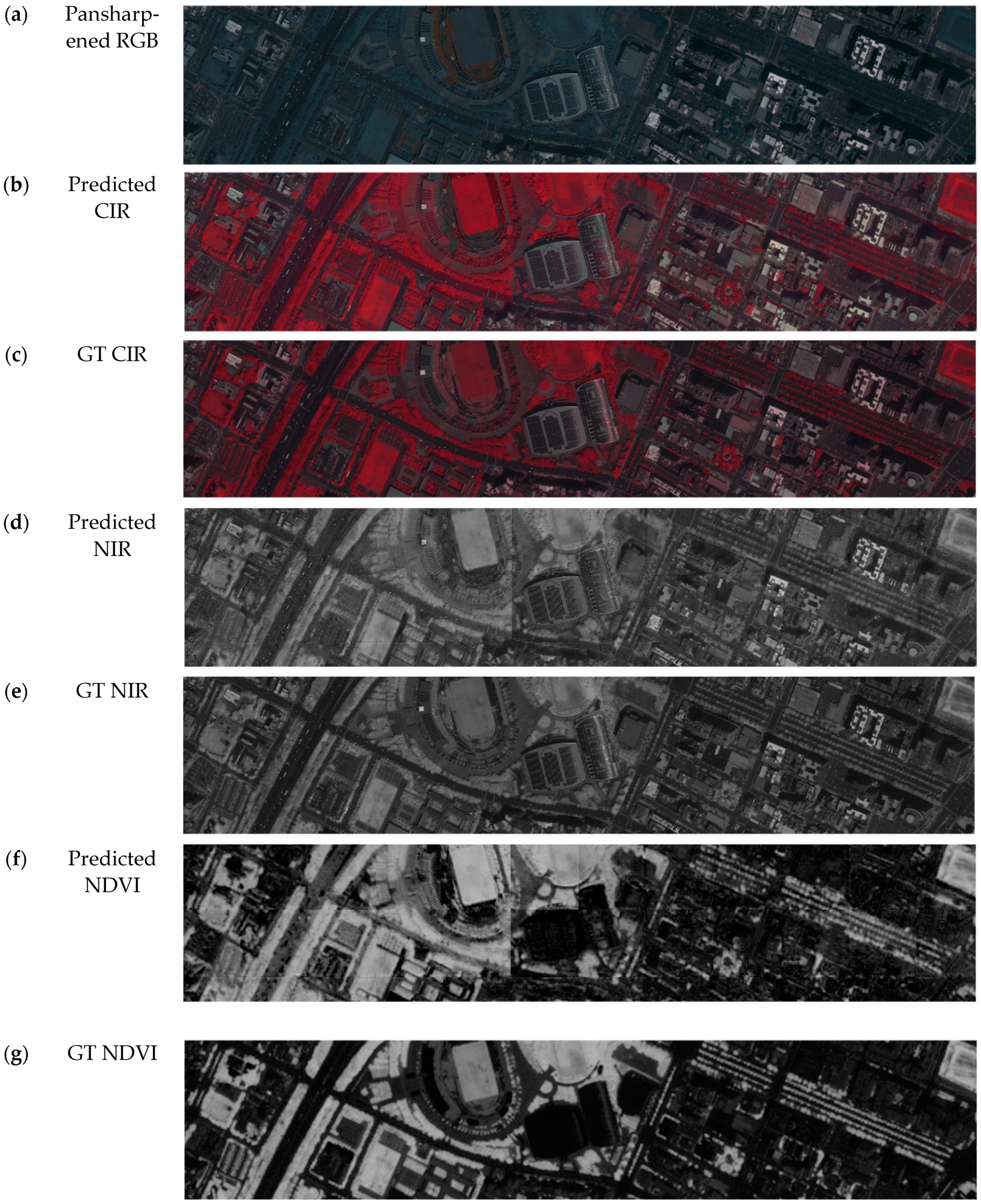
Figure 12.
Comparison between the prediction and the ground truth (GT) of the CIR, NIR and NDVI generated from a pansharpened RGB satellite sub-image.
Figure 12.
Comparison between the prediction and the ground truth (GT) of the CIR, NIR and NDVI generated from a pansharpened RGB satellite sub-image.
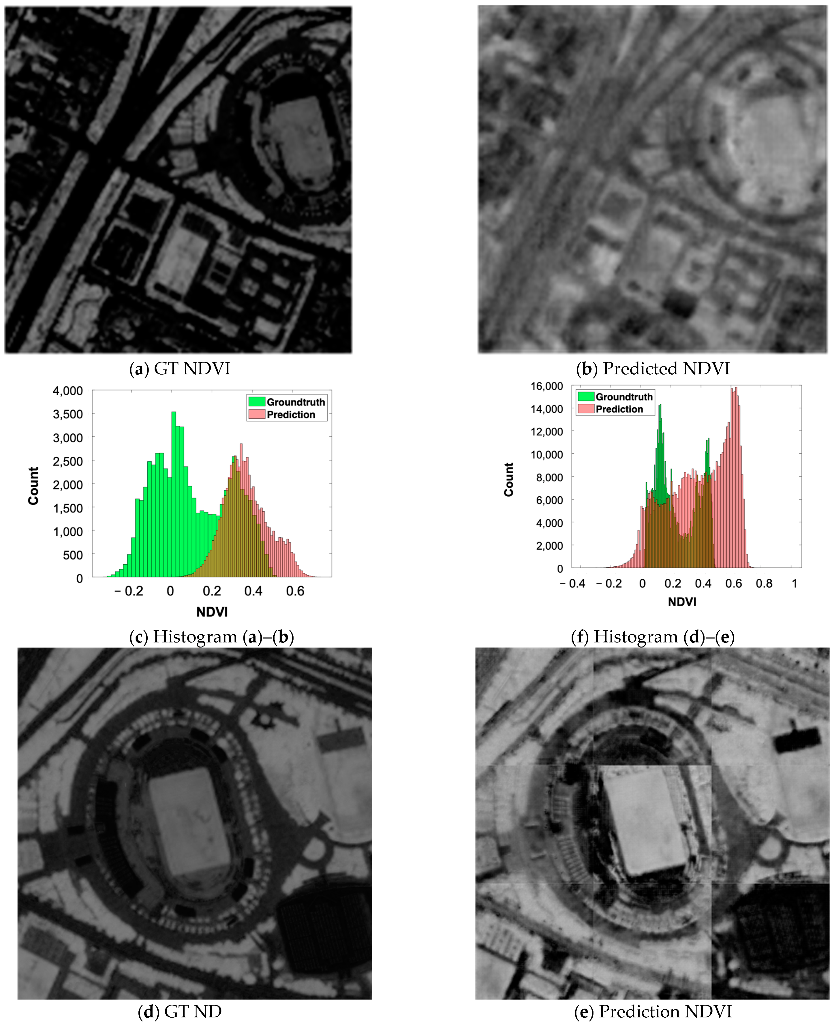
Figure 13.
Histogram and visual inspection of the CIR and NDVI simulated using MS and PAN images on the target stadium. (a–c) Ground truth (GT) and NDVI predicted using one tile with the size of 256 × 256 from MS Pleiades and their histograms. (d–f) Ground truth of CIR, NIR, NDVI and predicted NIR and NDVI images from nine tiles of the PAN Pleiades images and histograms for NDVI comparison.
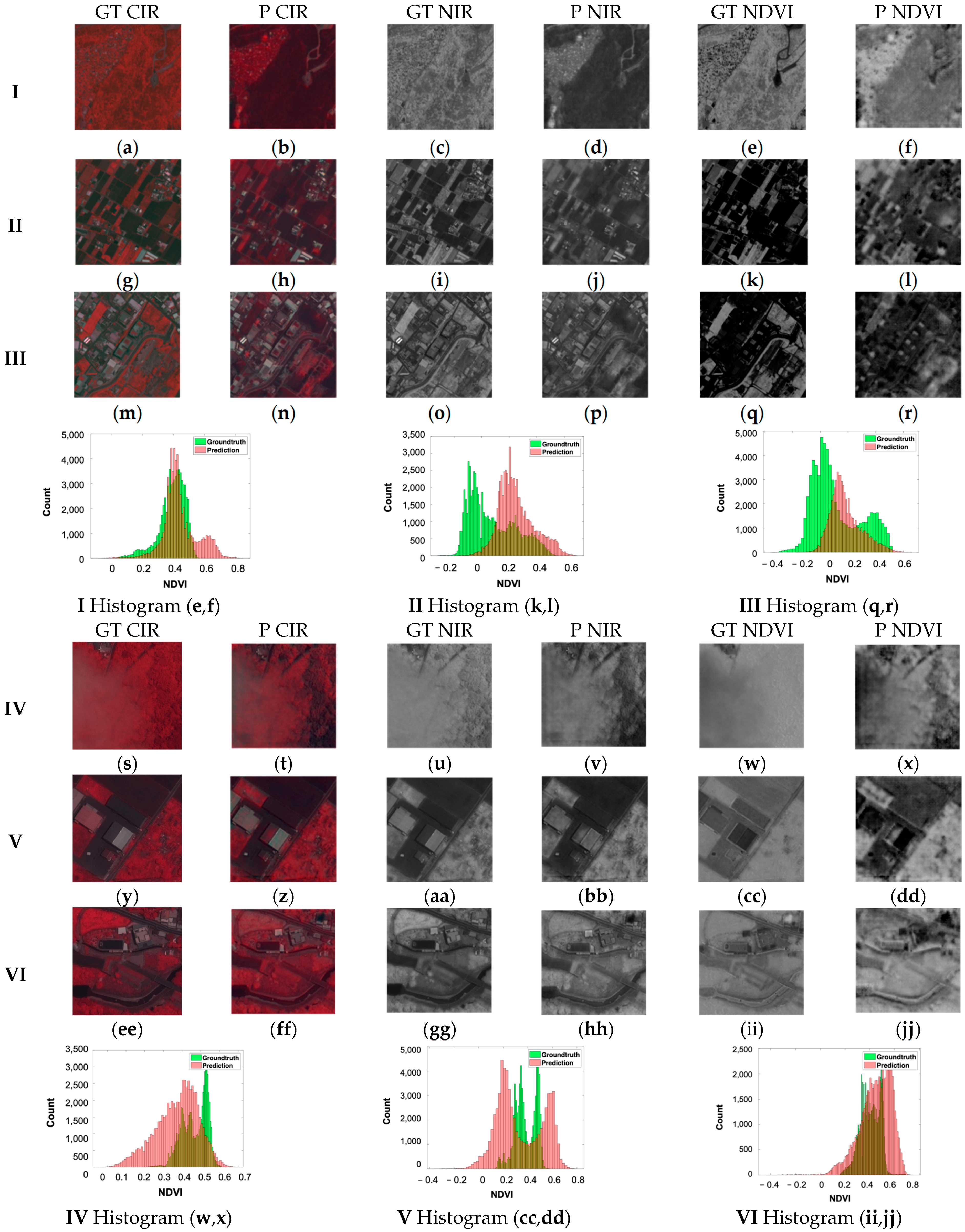
Figure 14.
Histogram and visual inspection of MS (I–III) and PAN (IV–VI) examples of Zhubei city.
Figure 14.
Histogram and visual inspection of MS (I–III) and PAN (IV–VI) examples of Zhubei city.
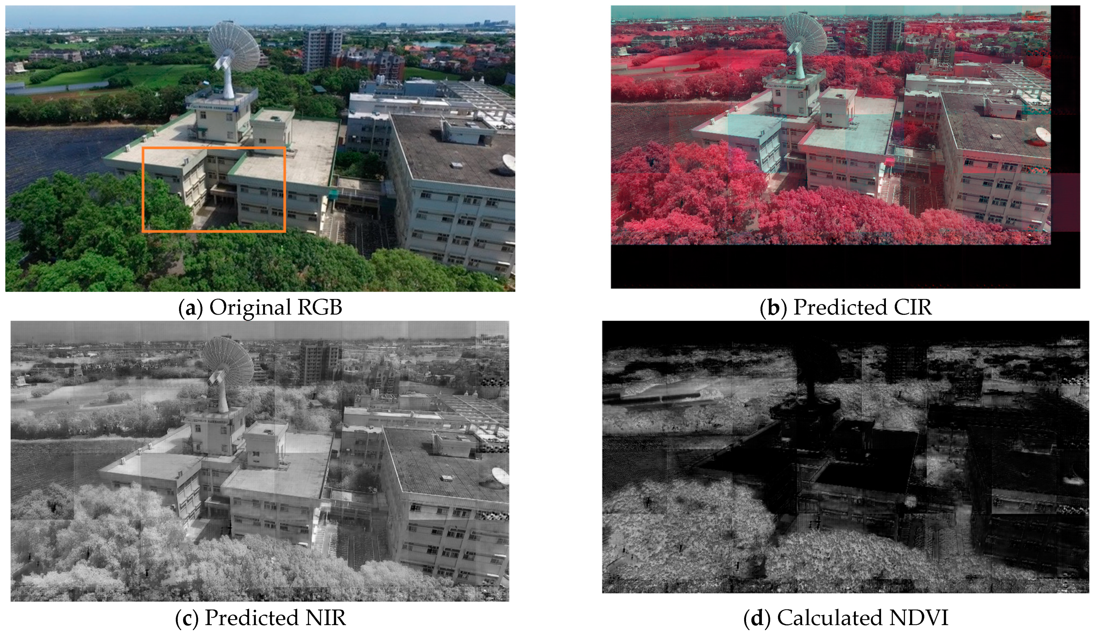
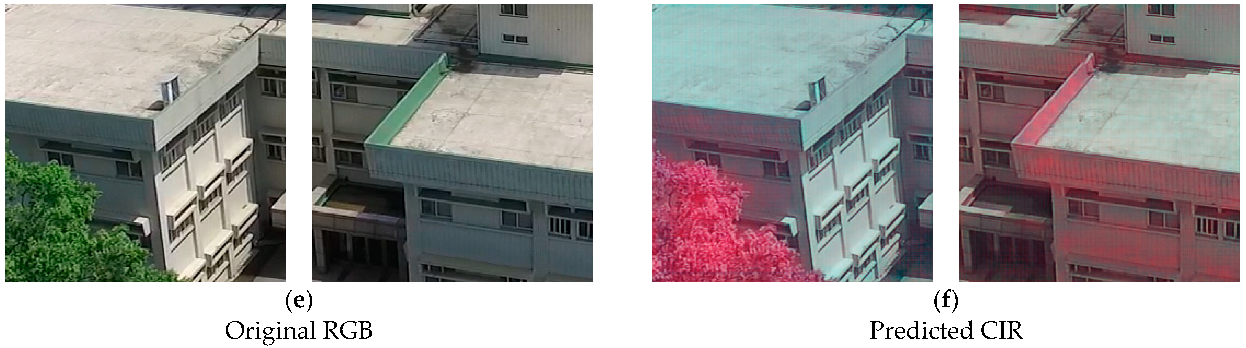
Figure 15.
Prediction of CIR, NIR and calculated NDVI of a UAV scene: (a) RGB, (b) predicted CIR image, (c) the extracted NIR band of (b), and (d) calculated NDVI with NIR and red band. A close-up view of the area marked with an orange box in (a) is displayed as two 256 × 256 tiles in RGB (e) and the predicted CIR (f).
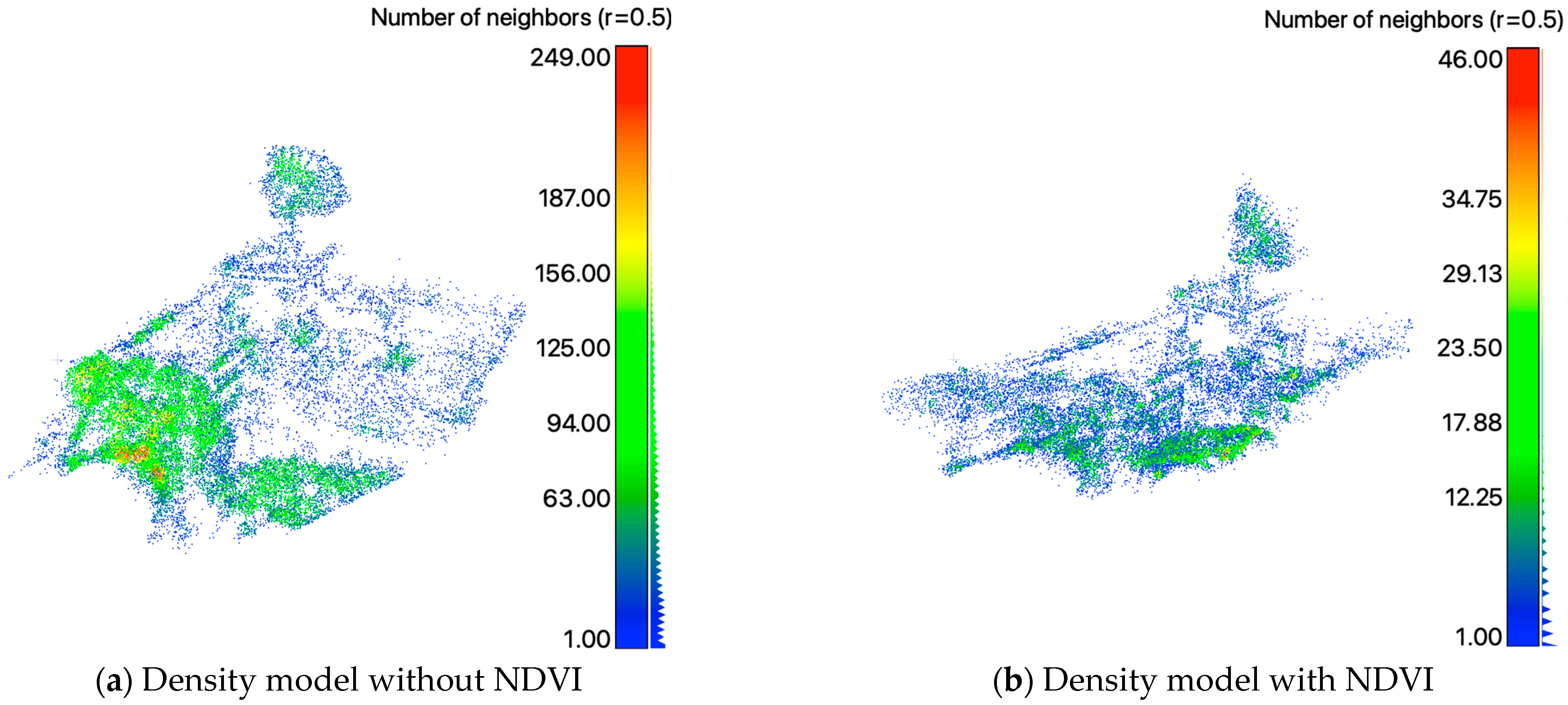
Figure 16.
Direct comparison between without (a) and with vegetation segmentation (b). Areas of low density shown in blue, areas of high density shown in red.
Figure 16.
Direct comparison between without (a) and with vegetation segmentation (b). Areas of low density shown in blue, areas of high density shown in red.
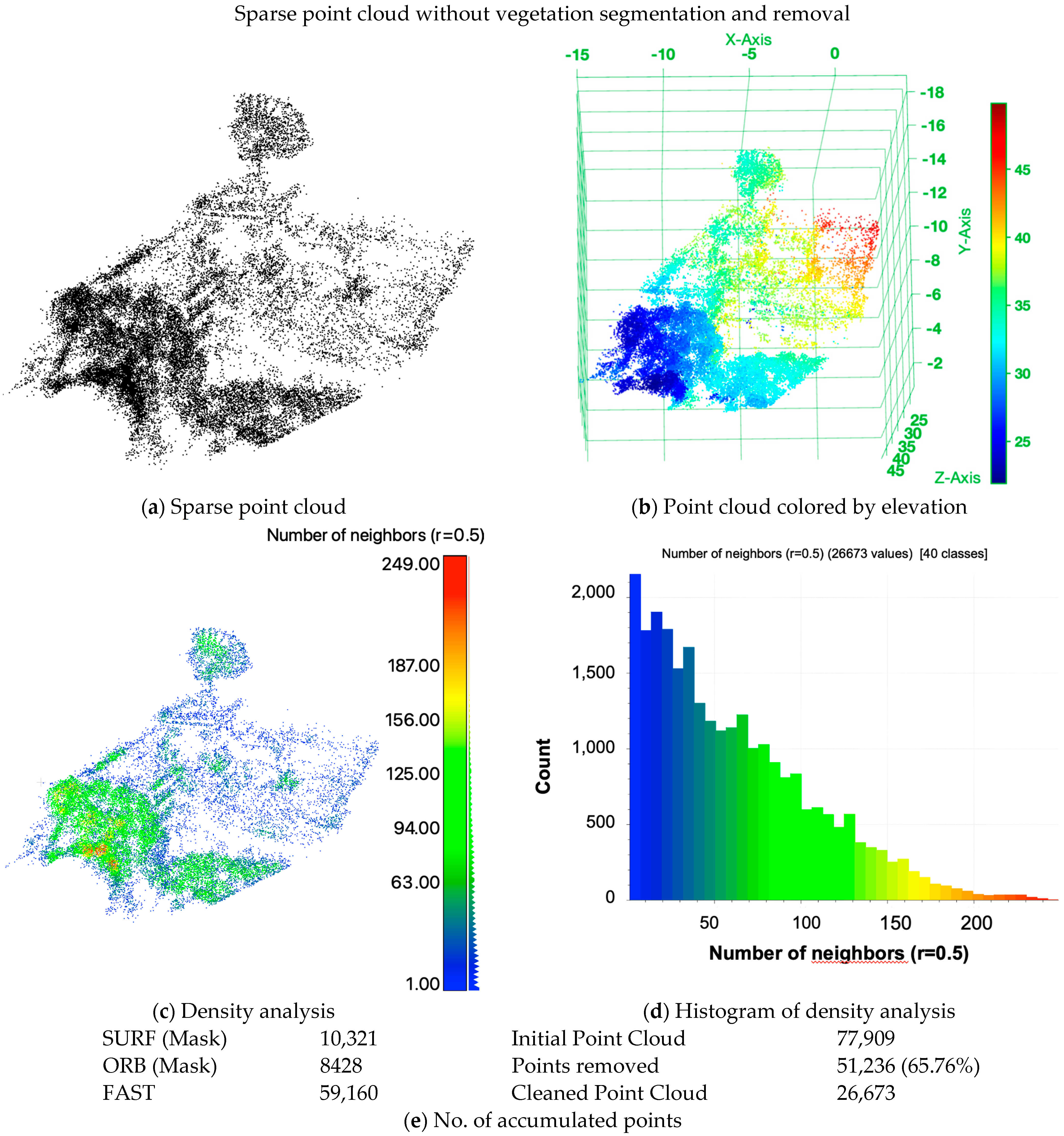
Figure 17.
Two−view SfM 3D sparse point cloud without the application of NDVI−based vegetation removal on the target CSRSR. (a) Sparse point cloud with no further coloring; (b) point cloud colored by elevation; (c) density analysis and the corresponding histogram (d). In addition, Table (e) shows the accumulated number of points over the three operators (SURF, ORB and FAST) and the initial and manually cleaned and processed point cloud.
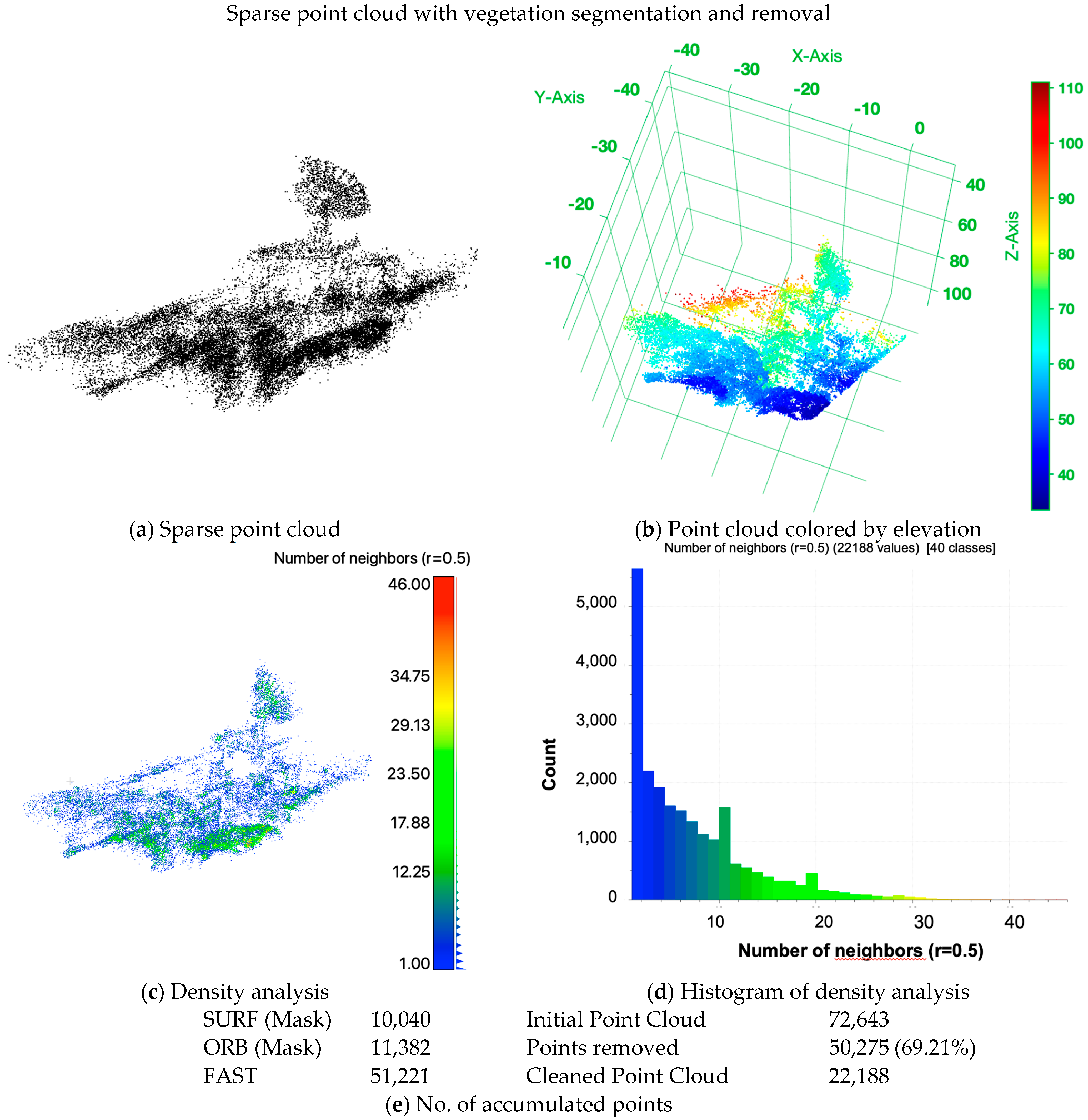
Figure 18.
Two−view SfM reconstructed 3D sparse point cloud with vegetation segmentation and removal process based on simulated NDVI of the target building. (a) Sparse point cloud with no further coloring; (b) point cloud colored by elevation; (c) density analysis and (d) the histogram. In addition, (e) lists the accumulated number of points over the three operators (SURF, ORB and FAST) after segmentation, with 0.5 NDVI as the threshold to mask vegetation in SURF and ORB, and the initial and manually cleaned point cloud.
Table 1.
EPFL RGB-NIR scene dataset. The categories in alphabetic order. In addition, the total number of images (RGB + NIR) and the number, respectively, of RGB and NIR.
Table 1.
EPFL RGB-NIR scene dataset. The categories in alphabetic order. In addition, the total number of images (RGB + NIR) and the number, respectively, of RGB and NIR.
| Category | | Category | | Category | |
|---|
| Country | 104 (52) | Indoor | 112 (56) | Street | 100 (50) |
| Field | 102 (51) | Mountain | 110 (55) | Urban | 116 (58) |
| Forest | 106 (53) | OldBuilding | 102 (51) | Water | 102 (51) |
Table 2.
Pleiades tri-stereo pairs including the view, the acquisition data and incident angle.
Table 2.
Pleiades tri-stereo pairs including the view, the acquisition data and incident angle.
| View | Date | Incident Angle |
|---|
| Nadir | 2019-08-27T | 12.57° |
| 9:18:44.807 |
| Forward | 2019-08-27T | 17.71° |
| 08:43:17.817 |
| Backward | 2019-08-27T | 16.62° |
| 08:47:06.900 |
Table 3.
The pre-processed available images. The Pleiades dataset consists of two groups, the multi-spectral (MS) and the panchromatic (PAN). The MS and EPFL data are processed with morphological changes (
Figure 6) to generate more tiles for training.
Table 3.
The pre-processed available images. The Pleiades dataset consists of two groups, the multi-spectral (MS) and the panchromatic (PAN). The MS and EPFL data are processed with morphological changes (
Figure 6) to generate more tiles for training.
| Pleiades | MS | PAN |
|---|
| | Size | Sliced | Tiles 1 | Tiles 2 | Total | Size | Sliced |
|---|
| Img1 (70) | 5285 × 5563 | 462 | 1386 | 7392 | 9240 | 21,140 × 22,250 | 7221 |
| Img2 (74) | 5228 × 5364 | 441 | 1322 | 7498 | 8820 | 20,912 × 21,452 | 6888 |
| Img3 (93) | 5189 × 5499 | 462 | 1386 | 7392 | 9240 | 20,756 × 21,992 | 7052 |
| EPFL | | | | | | | |
| Images | Tiles 1 | Tiles 2 | Tiles total | | | |
| 369 | 4452 | 17,808 | 22,260 | | | |
Table 4.
EPFL RGB-NIR dataset and training variation. There are 22,260 training tiles for 9 categories and around 50 h of training for 100 epochs. The table also shows training with only one (Streets) category (Training 1) and two (Streets and Forest) categories (Training 2). Tiles 1 and Tiles 2 are the products of the morphological changes described in
Figure 6.
| EPFL | Training 9 | Training 1 | Training 2 |
|---|
| Images | 369 | 16 | 32 |
| Tiles 1 | 4452 | 240 | 480 |
| Tiles 2 | 17,808 | 768 | 1536 |
| Tiles Total | 22,260 | 3840 | 7680 |
| Time | 50 h 48 min | 6 h 42 min | 13 h 1 min |
Table 5.
Training and testing for model selection.
Table 5.
Training and testing for model selection.
| | Overall | Streets | Streets, Forest | Streets, Forest, MS and PAN |
|---|
| Training Tiles | 22,260 | 3840 | 7680 | 15,360 |
| Numb. Categories | 9 | 1 | 2 | 4 |
| Time | 50 h 48 min | 6 h 42 min | 13 h 1 min | 25 h 51 min |
| EPFL RGB-NIR | 9 categories | 1 category | 2 categories | 2 categories |
| MS | × | × | × | 1 image |
| PAN | × | × | × | 1 image |
Table 6.
FID summary and CM for training model selection.
Table 6.
FID summary and CM for training model selection.
| | Street | Street and Forest | Street, Forest, MS and PAN |
|---|
| Model | 89 | 98 | 94 | 83 | 64 |
| CM | | | | | |
| Accuracy | 0.8136 | 0.5781 | 0.7645 | 0.6830 | 0.7125 |
| Precision | 0.7285 | 0.5423 | 0.6798 | 0.6120 | 0.6349 |
| F1-score | 0.8429 | 0.7033 | 0.8093 | 0.3660 | 0.4251 |
| Kappa | 0.6273 | 0.1563 | 0.5290 | 0.7593 | 0.7767 |
| FID | 1.132 | 3.057 | 0.839 | 1.663 | 1.905 |
Table 7.
Model testing for validation separating MS and PAN results. Pleiades MS and PAN, respectively, for the Forward (74) and Backward (93) view, including the average (AVG). In addition, the absolute Difference (Diff abs) and relative difference (Diff %) used to compare MS and PAN.
Table 7.
Model testing for validation separating MS and PAN results. Pleiades MS and PAN, respectively, for the Forward (74) and Backward (93) view, including the average (AVG). In addition, the absolute Difference (Diff abs) and relative difference (Diff %) used to compare MS and PAN.
| Pleiades | Accuracy | Recall | F1-Score | Kappa |
|---|
| MS74 | 0.5886 | 0.5486 | 0.7085 | 0.1772 |
| MS93 | 0.5956 | 0.5528 | 0.7120 | 0.1912 |
| AVG MS | 0.59 | 0.55 | 0.71 | 0.18 |
| PAN74 | 0.9466 | 0.9035 | 0.9493 | 0.8932 |
| PAN93 | 0.9024 | 0.8366 | 0.8048 | 0.9110 |
| AVG PAN | 0.92 | 0.87 | 0.88 | 0.90 |
| Diff abs | 0.33 | 0.32 | 0.17 | 0.72 |
| Diff % | 35.9 | 36.8 | 19.3 | 80 |
Table 8.
Number of points without or with the processing vegetation segmentation using the NDVI calculated using the NIR and red bands of the CIR image simulated from the original RGB UAV scene.
Table 8.
Number of points without or with the processing vegetation segmentation using the NDVI calculated using the NIR and red bands of the CIR image simulated from the original RGB UAV scene.
| Features | Initial | After | Difference |
|---|
| Image 1 | 148,717 | 133,186 | 15,531 | 10.44% |
| Image 2 | 149,646 | 134,430 | 15,216 | 10.17% |
| AVG | 149,181 | 133,808 | 15,373.5 | 10.31% |
Table 9.
Initial and cleaned sparse point cloud with and without NDVI-based vegetation segmentation and removal process.
Table 9.
Initial and cleaned sparse point cloud with and without NDVI-based vegetation segmentation and removal process.
| PCL | without NDVI | with NDVI | Difference |
|---|
| Initial | 77,909 | 72,643 | 5266 |
| Difference | 51,236 | 65.76% | 50,275 | 69.21% | 781 | 15.83% |
| Cleaned | 26,673 | 22,188 | 4485 |


