Laterally Excited Bulk Acoustic Wave Resonators with Rotated Electrodes Using X-Cut LiNbO₃ Thin-Film Substrates

Abstract

With the development of piezoelectric-on-insulator (POI) substrates, X-cut LiNbO₃ thin-film resonators with interdigital transducers are widely investigated due to their adjustable resonant frequency (f_s) and effective electromechanical coupling coefficient ($K_{eff}^2$). This paper presents an in-depth study of simulations and measurements of laterally excited bulk acoustic wave resonators based on an X-cut LiNbO₃/SiO₂/Si substrate and a LiNbO₃ thin film to analyze the effects of electrode angle rotation ($\theta$) on the modes, f_s, and $K_{eff}^2$. The rotated $\theta$ leads to different electric field directions, causing mode changes, where the resonators without cavities are longitudinal leaky SAWs (LLSAWs, $\theta$ = 0$°$) and zero-order shear horizontal SAWs (SH₀-SAWs, $\theta$ = 90$°$) and the resonators with cavities are zero-order-symmetry (S₀) lateral vibrating resonators (LVRs, $\theta$ = 0$°$) and SH₀ plate wave resonators (PAW, $\theta$ = 90$°$). The resonators are fabricated based on a 400 nm X-cut LiNbO₃ thin-film substrate, and the measured results are consistent with those from the simulation. The fabricated LLSAW and SH₀-SAW without cavities show a $K_{eff}^2$ of 1.62% and 26.6% and a Bode-Q_max of 1309 and 228, respectively. Meanwhile, an S₀ LVR and an SH₀-PAW with cavities present a $K_{eff}^2$ of 4.82% and 27.66% and a Bode-Q_max of 3289 and 289, respectively. In addition, the TCF with a different rotated $\theta$ is also measured and analyzed. This paper systematically analyzes resonators on X-cut LiNbO₃ thin-film substrates and provides potential strategies for multi-band and multi-bandwidth filters.

1. Introduction

With the rapid development of technology, innovations and breakthroughs in wireless communication technology are also constantly occurring. Fifth-generation (5G) mobile communication technology provides stronger support for future applications such as digitization, intelligence, and networking [1]. With the continuous development of communication, the division of communication frequency bands is becoming increasingly refined and complex; therefore, the requirements for the diversity and performance of radio-frequency (RF) components such as filters are also increasing. The demand for integrating multi-band and multi-bandwidth filters in limited space is increasing.

Lithium niobate (LiNbO₃) piezoelectric materials have significant differences in piezoelectric properties due to their crystal properties, and materials with different tangential directions also exhibit significant variations in their piezoelectric properties [1]. Thanks to the development and widespread application of ion-slicing technology, LiNbO₃ piezoelectric materials are gradually being applied in filters [2,3,4,5,6,7,8,9,10,11]. There are many studies on the LiNbO₃ substrate with different tangential directions [12,13,14,15,16,17,18,19,20,21]. Resonators based on the Z-cut LiNbO₃ thin film are commonly used at high frequencies and wide bandwidths due to their large piezoelectric coefficient e₁₆. The laterally excited bulk acoustic wave resonator (XBAR) based on a Z-cut LiNbO₃ substrate exhibits an excellent electromechanical coupling coefficient (K²) larger than 20% when operating at 5 GHz [22,23,24]. Other types of resonators based on LiNbO₃ substrates have also been extensively studied. Fabricated film bulk acoustic resonators (FBARs) using a Y+36°-cut LiNbO₃ substrate working at 4.7 GHz and with an effective electromechanical coupling coefficient ($K_{eff}^2$) of 25% and a quality factor at anti-resonance of 574 have been reported [6]. One study of resonators based on rotated Y-cut LiNbO₃ on the K² of the shear horizontal (SH) mode showed that the largest K² is 15% [25].

In recent years, the resonators with LiNbO₃ plates bonded on different substrates such as silicon carbide (SiC) have attracted great interest [26,27,28,29,30]. Generally, silicon (Si) substrates are also typically chosen as long as they are low cost and can support the confined propagation of surface acoustic waves (SAWs) in LiNbO₃ due to the sharp contrast of material properties between Si and LiNbO₃. A study on the SAWs on a 15$°$YX-LiNbO₃/SiO₂/Si substrate presented a high K² ranging from 22.5% to 25.2% [31]. S₀ mode laterally vibrating resonators (LVRs) on an X-cut LiNbO₃ substrate operating between 100 MHz and 1 GHz have been widely investigated [32]. But there is still an urgent need for systematic research on resonators based on X-cut LiNbO₃ thin-film substrates that meet the needs of wideband filtering.

In this paper, the performance of the resonators based on an X-cut LiNbO₃ thin film based on an X-cut LiNbO₃/SiO₂/Si substrate and a LiNbO₃ thin film are investigated. The mode, resonant frequencies, and the $K_{eff}^2$ of different modes corresponding to resonators with different angle rotations ($\theta$) were carefully studied and analyzed. Further simulation analyses were conducted on the resonant main modes corresponding to resonators with different values of $\theta$. The fabricated devices are systematically compared, and the simulation results are summarized. In addition, in this article, we also study the TCF of resonators under different values of $\theta$.

2. Modeling and Simulation

2.1. Device Modeling

The vertical view of the resonator with an interdigital transducer electrode (IDT) in the xy-plane is shown in Figure 1a, where the main geometric parameters of the resonator are marked. WE and L_e are the width and length of the electrode. The gap (G) is the distance between the electrode and the busbar. The pitch (P) is the center distance between adjacent electrodes. The angle at which the arrangement direction of the forks rotates counterclockwise along the y-axis is defined as $\theta$. The resonator based on an X-cut LiNbO₃/SiO₂/Si substrate without a cavity, shown in Figure 1c, consists of a metal layer, a thin monocrystalline LiNbO₃ layer, and a SiO₂ layer supported by the Si substrates, while the resonator based on an X-cut LiNbO₃ thin film with a cavity only consists of the metal layer and a thin-film piezoelectric layer, without SiO₂ and Si as substrates. In addition, h_Mo, h_LN, and h_SiO2 represent the thickness of the metal layer, the LiNbO₃ thin film, and the SiO₂ layer, respectively.

The finite element simulation method (FEM) using COMSOL6.0 software is adopted in this article to simulate the dispersion characteristics of the resonators on an X-cut LiNbO₃ thin film and the effects of h_LN and $\theta$ on the resonant frequency. Periodic boundary conditions in the propagation direction (x-direction) and shear horizontal direction (y-direction) are applied.

The dispersive diagram for propagation on the x-axis for the real part of the propagation constants (kx) is shown in Figure 2a. The dispersion curve presented in Figure 2a is different from that for Lamb waves, since the curve includes kx = 0 m⁻¹ but also all multiples of pi/P. Figure 2b shows the total displacements of different mode shapes while kx = 0 m⁻¹. Mode I and the mode II are the first-order anti-symmetric (A₁) modes. Mode III and mode IV are the lateral vibration (LV) modes. The displacements of mode I have no shear displacement, which is different from the displacement of the main mode of the XBAR based on a Z-cut LiNbO₃ thin film. Mode V and mode VI are the higher-order anti-symmetric modes, which are the third order antisymmetric mode (A₃). One mode corresponds to two eigenfrequencies. A pair of eigenfrequencies of a mode represent the two edges of the bandgap. The displacements of this pair of eigenfrequencies are symmetric and asymmetric about the centerline, respectively. The appearance of the symmetric modes is due to constructive interference between two waves propagating in the opposite directions at one edge of the bandgap, causing resonance. The appearance of anti-symmetric modes is due to their destructive interference at the other edge of the bandgap, causing anti-resonance.

In this paper, the modes of the resonator are analyzed firstly. Figure 3a–d show the four main modes in the SAW resonators based on an X-cut LiNbO₃/SiO₂/Si substrate, corresponding to the Rayleigh, the zero-order shear horizontal (SH₀), the first-order shear horizontal (SH₁), and the longitudinal leaky (LL), respectively. The FEM is adopted in this article to simulate the effects of h_LN and $\theta$ on resonant frequency. Figure 3e shows the variation in the four modes’ frequencies with the variation in the h_LN, while the WE is fixed at 1 μm and the P is 2 $\mathsf{\mu }\mathrm{m}$. From the graph, we can see that for the SH₀-SAW resonators, the resonant frequencies of the SH₀ mode and Rayleigh mode are always very close regardless of the h_LN. This makes it important to suppress the Rayleigh mode for the SH₀-SAW resonators. As the h_LN/$\lambda$ increases (the $\lambda$ is the wavelength), the resonant frequencies of the SH₀ mode show a slow upward trend but remain in the low-frequency range below 1 GHz. The resonant frequencies of the higher-order modes (the SH₁ mode and the LL mode) are always above 1 GHz. Figure 3f reveals that the patterns of the simulated frequencies of the four modes vary with the $\theta$ of the resonators in the yz-plane, while the h_LN/$\lambda$ is fixed at 0.1. The horizontal setting of the IDTs in the yz-plane is defined as the initial value, with a $\theta$ of 0$°$. When the $\theta$ varies from 0$°$ to 180$°$, the frequencies of the SH₀ resonators exhibit periodic changes. The resonant frequency reaches the highest value at a $\theta$ of 50$°$ and 140$°$. As the $\theta$ increases from 0$°$ to 50$°$, the resonant frequency of the SH₀ mode increases and then gradually decreases as the $\theta$ further increases to 90$°$. The SH₁ mode and the SH₀ mode have similar patterns of variation, while the frequency response of the Rayleigh waves is not sensitive to changes in the $\theta$. For the LL mode, its maximum frequency response occurs when the $\theta$ is 0$°.$

Figure 4a–d show the four main modes of resonators based on an X-cut LiNbO₃ thin film with cavities, corresponding to the zero-order anti-symmetry (A₀) mode, the zero-order symmetry (S₀) mode, the SH₀ mode, and the shear vertical (SV) mode, respectively. Figure 4e shows the resonant frequencies’ variation in the four modes with the different values of h_LN/$\lambda$, while the WE is fixed at 1 $\mathsf{\mu }\mathrm{m}$ and the P is 2 $\mathsf{\mu }\mathrm{m}$. For the resonators with the SH₀ mode, as the h_LN increases, the resonance frequencies’ variation in the SH₀ mode is not significant, but the resonance frequencies’ variation in the A₀ mode will gradually cause interference with the main resonance of the resonators. The frequencies’ variation in the S₀ mode with the different values of h_LN/$\lambda$ are consistent with these of the SH₀ mode, except that the frequencies are slightly higher. When h_LN/$\lambda$ increases to a certain level, the SV mode cannot be excited.

Figure 4f shows that the patterns of the simulated frequencies of the four modes vary with the $\theta$, while the h_LN/$\lambda$ is fixed at 0.1. The frequencies of the SH₀ mode exhibit periodicity as the $\theta$ changes from 0$°$ to 180$°$, while the frequencies of the A₀ mode have little effect on the change in the $\theta$. The resonant frequency reached the highest value when the $\theta$ = 50$°$ and $\theta$ = 140$°$. As the $\theta$ increases from 0$°$ to 50$°$, the resonant frequency corresponding to the SH₀ mode increases and then gradually decreases as the $\theta$ further increases to 90$°$. For the resonators with the S₀ mode, the maximum value of frequency occurs when the $\theta$ = 90$°$. The SV mode can be excited at relatively high frequencies and maintains a certain difference from the main mode (S₀) as the angle changes. Therefore, we can design the resonant frequency by rotating it without increasing the difficulty and complexity of the process, which provides new ideas for the design of filters.

2.2. Analysis of Rotation Angle

When the resonator rotates in the horizontal yz -plane, its performance changes accordingly, which is a noteworthy aspect of the resonator’s design on the X-cut LiNbO₃ thin-film substrates. The FEM using COMSOL6.0 software is used for a simulation analysis and selected a 400 nm thick LiNbO₃ thin film and a 200 nm thick Mo electrode. The thickness of the SiO₂ is 3 $\mathsf{\mu }\mathrm{m}$, and there is a perfect matching layer under the Si substrate. In this part, the influence of the geometric structural parameters of the two types of resonators based on the X-cut LiNbO₃ thin-film substrates on the resonant frequency and $K_{eff}^2$ are investigated. The $K_{eff}^2$ is calculated by the series resonant frequency (f_s) and parallel resonant frequency (f_p), as follows [33]:

$$K_{eff}^2={\displaystyle \frac{{\pi }^2}{4}}(f_s(f_p-f_s))/{f_p}^2$$

(1)

When the resonator rotates in the horizontal yz-plane, its performances change accordingly, which is a noteworthy aspect of the X-cut LiNbO₃ thin-film substrates. For resonators based on an X-cut LiNbO₃/SiO₂/Si substrate, when the IDT electrodes are horizontally distributed along the y-axis (while $\theta$ = 0$°$), the main mode of the resonator is the LL mode. As shown in Figure 5a, when the $\theta$ gradually increases from 0$°$ to 70$°$ (with a fixed WE = 1 $\mathsf{\mu }\mathrm{m}$, P = 2 $\mathsf{\mu }\mathrm{m}$, h_LN/$\lambda$ = 0.2, and h_SiO2/$\lambda$ = 0.75), the main mode is unchanged but the f_s gradually decreases, and the f_p does not change much. At this time, the electromechanical conversion efficiency increases. When the $\theta$ increases to 40$°$, the parasitic mode next to the main mode has a greater impact on the resonator, which is worth noting in resonator design. It can be seen from Figure 5b that when the $\theta$ increases to 80$°$, the main mode changes to the SH₀ mode. When the $\theta$ further increases from 80$°$ to 130$°$, the main mode of the resonator remains in the SH₀ mode, but the f_s decreases firstly and then increases, while the f_p remains unchanged. Therefore, according to the previous formula, the $K_{eff}^2$ increase firstly and then decrease. In Figure 5c, when the $\theta$ further increases to 140$°$, the main resonant mode returns to the LL mode. As the $\theta$ gradually increases from 140$°$ to 170$°$, the f_s of the resonator gradually increases and the $K_{eff}^2$ of the resonator does not change much.

For the resonators based on the X-cut LiNbO₃ thin film with cavities, as the $\theta$ changes, its resonant mode is the SH₀ mode or the S₀ mode. When the $\theta$ is 0$°$, the main mode of the resonator is the S₀ mode. As shown in Figure 6a, when the $\theta$ gradually increases from 0$°$ to 60$°$ (with a fixed WE = 1 $\mathsf{\mu }\mathrm{m}$, P = 2 $\mathsf{\mu }\mathrm{m}$, h_LN/$\lambda$ = 0.2, and h_SiO2/$\lambda$ = 0.75), the main mode remains unchanged, but the f_s gradually decreases and the f_p does not change much. At this time, the $K_{eff}^2$ increases. In Figure 6b, when the $\theta$ increases to 70$°$, the main mode of the resonator is the SH₀ mode, and the operating frequency is less than 1 GHz. At this point, the resonator has a parasitic mode (S₀) at higher frequencies. When the $\theta$ further increases from 70$°$ to 130$°$, the main mode of the resonator remains in the SH₀ mode, but the f_s decreases first and then increases, and the $K_{eff}^2$ increase firstly and then decrease. As shown in Figure 6c, when the $\theta$ is 100$°$, the $K_{eff}^2$ reaches its maximum value. As the $\theta$ further increases, it gradually increases from 140$°$ to 170$°$, and the main mode of the resonator switches back to the S₀ mode. The f_s of the resonators decrease as the $\theta$ increases.

Figure 7a,b show the f_s and $K_{eff}^2$ of the resonators based on an X-cut LiNbO₃/SiO₂/Si substrate and a LiNbO₃ thin-film substrate when the $\theta$ changes from 0$°$ to 180$°$; the black corresponds to the SAW resonators with an X-cut LiNbO₃/SiO₂/Si substrate and the red corresponds to the resonators with an X-cut LiNbO₃ thin-film substrate. The corresponding specific data are presented in

Table 1. The f_s and (b) $K_{eff}^2$ of the resonator without a cavity when the $\theta$ changes from 0$°$ to 180$°$.

$\mathit{\theta }$ (°) 1	0	10	20	30	40	50	60	70	80
fs (GHz) 2	1.31	1.3	1.28	1.27	1.25	1.22	1.25	1.26	0.773
${\mathit{K}}_{\mathit{e}\mathit{f}\mathit{f}}^2$ (%) 3	3.71	3.74	5.65	7.53	11.3	18.69	13.08	11.22	13.57
$\mathit{\theta }$ (°) 1	90	100	110	120	130	140	150	160	170
fs (GHz) 2	18.05	20.81	20.56	14.69	5.95	3.77	5.61	3.74	3.71
${\mathit{K}}_{\mathit{e}\mathit{f}\mathit{f}}^2$ (%) 3	30	32.9	29.22	19.48	12.99	4.11	4.08	4.04	4.01

¹ $\theta$ is the rotation angle of the resonators; ² f_s is the series resonant frequency; ³ $K_{eff}^2$ is the effective electromechanical coupling coefficient of the resonators.

and

Table 2. The f_s and (b) $K_{eff}^2$ of the resonator with a cavity when the $\theta$ changes from 0$°$ to 180$°$.

$\mathit{\theta }$ (°) 1	0	10	20	30	40	50	60	70	80
fs (GHz) 2	1.21	1.2	1.18	1.15	1.12	1.1	1.1	0.7	0.67
${\mathit{K}}_{\mathit{e}\mathit{f}\mathit{f}}^2$ (%) 3	4.01	6.02	8.09	12.24	18.35	24.27	24.07	10.14	20.28
$\mathit{\theta }$ (°) 1	90	100	110	120	130	140	150	160	170
fs (GHz) 2	0.65	0.65	0.67	0.7	0.72	1.18	1.19	1.2	1.21
${\mathit{K}}_{\mathit{e}\mathit{f}\mathit{f}}^2$ (%) 3	30	32.9	29.22	19.48	12.99	4.11	4.08	4.04	4.01

¹ $\theta$ is the rotation angle of the resonators; ² f_s is the series resonant frequency; ³ $K_{eff}^2$ is the effective electromechanical coupling coefficient of the resonators.

. For the SAW resonators with an X-cut LiNbO₃/SiO₂/Si substrate, when the $\theta$ is between 0$°$ and 70$°$, the f_s of the resonators is significantly higher than that when the $\theta$ is between 80$°$ and 130$°$, which is maintained above 1 GHz. This is because within this range the main mode of the resonator is the LL mode. The $K_{eff}^2$ of the SAW resonators increase with the increase in the $\theta$. When the $\theta$ is 50$°$, the sudden increase in $K_{eff}^2$ is due to the disturbance of the parasitic modes. When the $\theta$ is between 80$°$ and 130$°$, due to the change of the main resonant mode to the SH₀ mode, which has a low sound velocity, the f_s decreases. The $K_{eff}^2$ increase firstly and then decrease as the $\theta$ increase. When the $\theta$ is 100$°$, the $K_{eff}^2$ reaches its maximum value, which is 20.81%. As the $\theta$ increases from 130$°$ to 180$°$, the f_s of the resonators is above 1 GHz, and as the $\theta$ increases, both f_s and $K_{eff}^2$ of the resonators remain relatively constant. For the resonators with an X-cut LiNbO₃ thin-film substrate, similar to the SAW resonators, when the $\theta$ is between 0$°$ and 60$°$, the f_s of the resonators are significantly higher than that when $\theta$ is between 70$°$ and 130$°$. The f_s of the resonators are above 1 GHz because the main mode of the resonator is the S₀ mode. The $K_{eff}^2$ of the resonators increase with the increase in the $\theta$. When the $\theta$ is between 70$°$ and 130$°$, due to the change of the main mode to the SH₀ mode, which has a low sound velocity, the f_s decrease. The $K_{eff}^2$ increase firstly and then decrease as the $\theta$ increase. When the $\theta$ is 100$°$, the $K_{eff}^2$ reaches its maximum value, which is 32.9%. As the $\theta$ increase from 130$°$ to 180$°$, the f_s of the resonators are above 1 GHz. At this stage, the $\theta$ has little effect on the f_s and the $K_{eff}^2$. The f_s of the resonators with an X-cut LiNbO₃ thin-film substrate are generally lower than that of the resonators with an X-cut LiNbO₃/SiO₂/Si substrate, but the $K_{eff}^2$ are larger than the $K_{eff}^2$ of the resonators with an X-cut LiNbO₃/SiO₂/Si substrate.

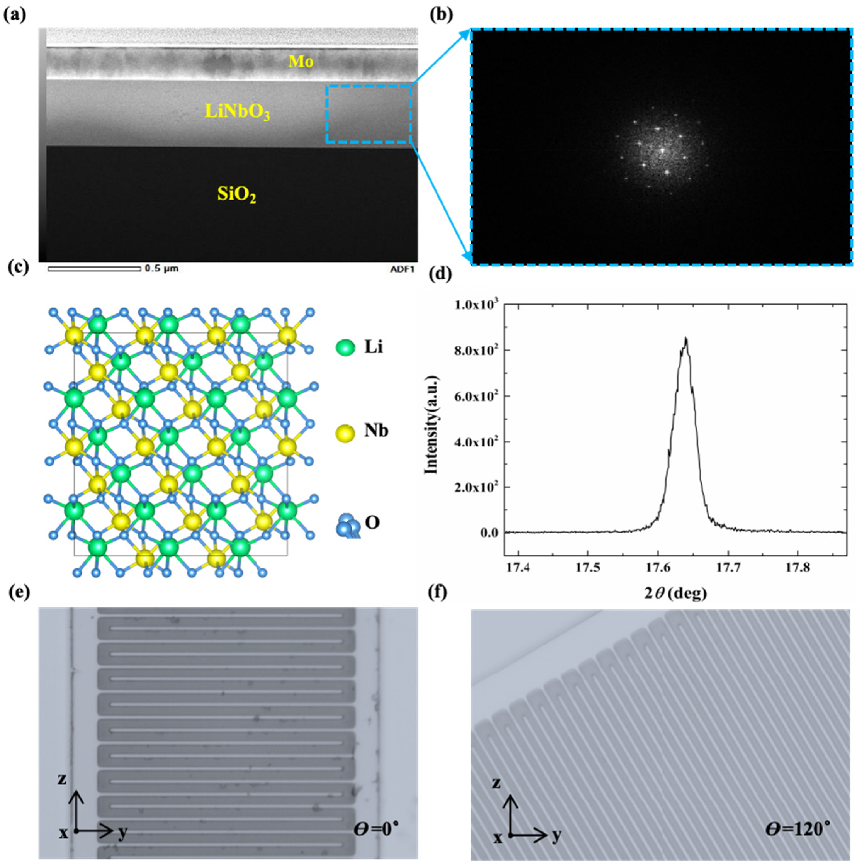
3. Fabrication and Characterization

The fabrication process flow is illustrated in Figure 8a–d. The top electrode is a 200 nm-thick Mo layer to reduce the electrical loss of the electrodes, and the electrode was patterned using the ion beam etching (IBE) method. Later, the deep reactive ion etching (DRIE) method was used to suspend the resonators, and then we controlled the time precisely to remove the SiO₂ by the buffered oxide etching (BOE) method.

The cross-sectional scanning electron microscope (SEM) images are shown in Figure 9a. The picture in Figure 9b is the transmission electron microscope (TEM) image in the X-cut LiNbO₃. A schematic diagram of the unit cell of the X-cut LiNbO₃ is shown in Figure 9c, and the measured X-ray diffraction (XRD) spectrum of the LiNbO₃ film is shown in Figure 9d. The optical images of the devices of a LiNbO₃/SiO₂/Si membrane with IDTs having dimensions of pitch of 2 $\mathsf{\mu }\mathrm{m}$ and electrode width of 1 $\mathsf{\mu }\mathrm{m}$ are shown in Figure 9e,f. The devices were fabricated on a 400 nm-thick X-cut LiNbO₃/SiO₂/Si substrate. The three-layer structure of the LiNbO₃ on isolation (LNOI) wafer is 400 nm-thick LiNbO₃, 3 $\mathsf{\mu }\mathrm{m}$-thick SiO₂, and 725 $\mathsf{\mu }\mathrm{m}$-thick Si, respectively.

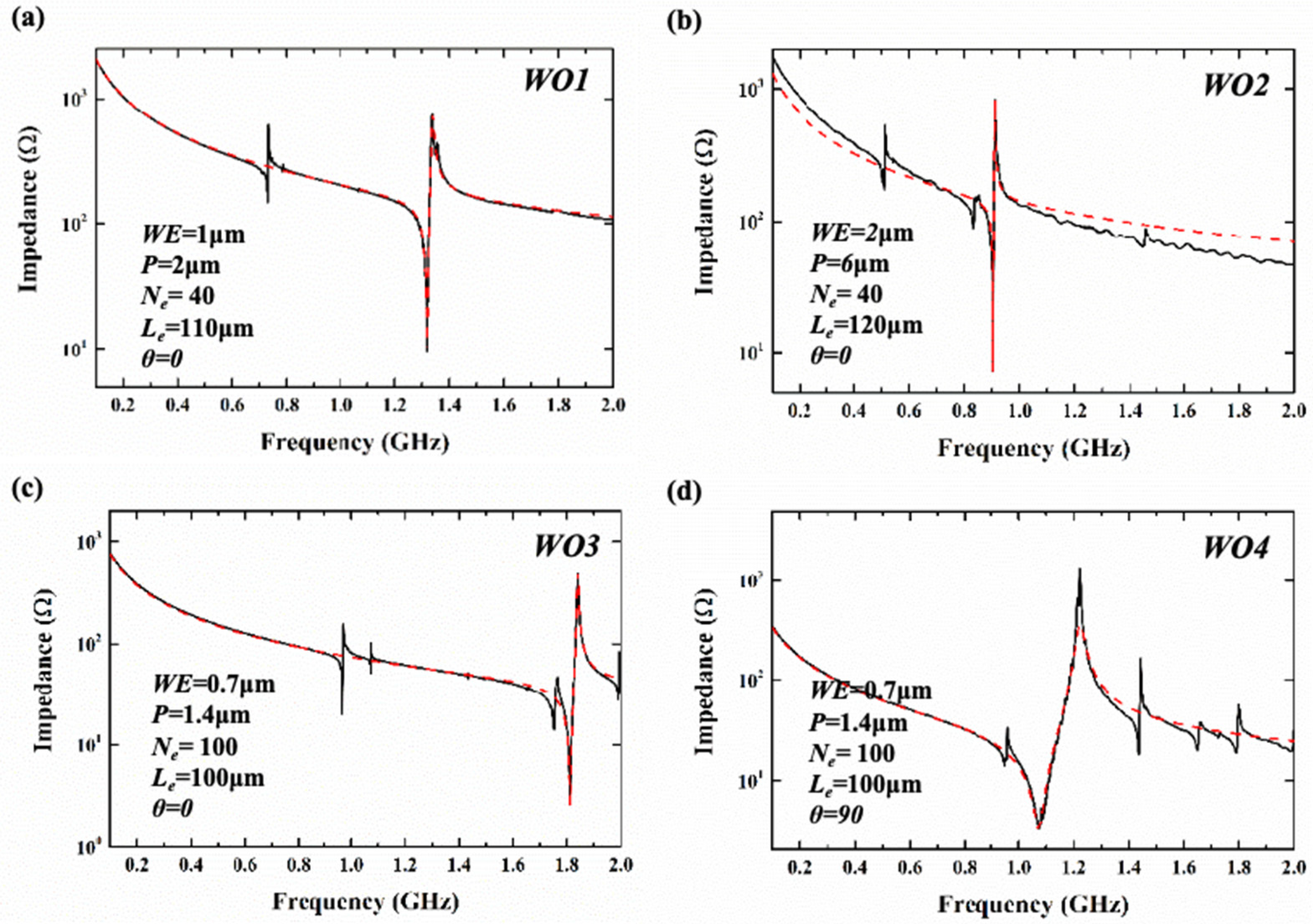
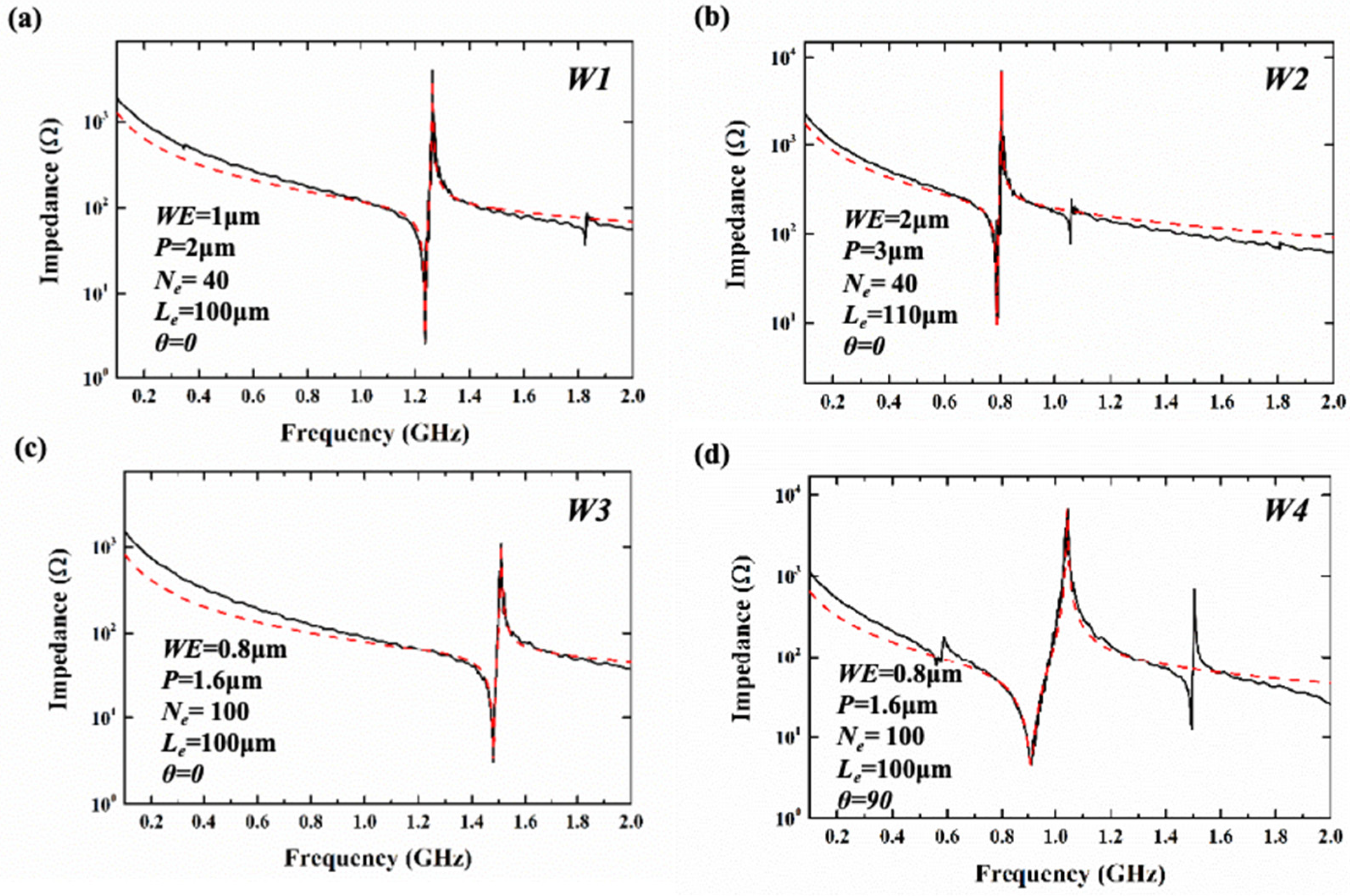
3.1. Impedance Curve and MBVD Model Fitting

With a ground–signal–ground (GSG) probe and an Agilent N5222B vector network analyzer platform, the S parameters (S₁₁) of the resonators were measured and later converted to impedance via software. Figure 10 and Figure 11 show the corresponding measured impedance curves and Modified Butterworth–Van Dyke (MBVD) modal fitting curves of the resonators based on the two types of substrates. Finally, the $K_{eff}^2$, the static capacitance (C₀), the maximum of Bode-Q (Bode-Q_max), and the resistance parameters were extracted and are displayed in

Table 3. Performance of fabricated devices with LNOI substrate.

Resonator	WO1	WO2	WO3	WO4
Mode	LLSAW	LLSAW	LLSAW	SH0-SAW
fs (GHz)	1.319	0.904	1.812	1.074
$K_{eff}^2$ (%)	3.45	1.62	3.70	26.60
Bode-Qmax	708	1309	705	228
C0 (pF)	0.736	1.197	2.06	3.641
R0 $(\mathsf{\Omega }$)	27	19.55	1.3	1.5
RS $(\mathsf{\Omega }$)	0.408	0.65	0.4	1.2
RM $(\mathsf{\Omega }$)	9.31	6.6	2.2	2

and

Table 4. Performance of fabricated devices with an X-cut LiNbO₃ thin film.

Resonator	W1	W2	W3	W4
Mode	S0	S0	S0	SH0
fs (GHz)	1.237	0.787	1.48	0.91
$K_{eff}^2$ (%)	5.16	4.82	4.65	27.66
Bode-Qmax	1237	803	740	288
C0 (pF)	1.202	0.876	1.881	1.87
R0 $(\mathsf{\Omega }$)	1.9	1.4	0.76	0.5
RS $(\mathsf{\Omega }$)	1.1	3.65	1	0.48
RM $(\mathsf{\Omega }$)	1.4	5.99	2.12	4.1

. The Bode-Q is evaluated using the following equation [29]:

$$Q_{B\text{ode}}=\omega · |S_{11}| · {\displaystyle \frac{GD\left(S_{11}\right)}{1-\left|\mathrm{S}11\right|}}$$

(2)

where the ω represents the angular frequency, the S₁₁ is the one port scattering parameter, and GD(S₁₁) is the group delay derived from S₁₁. The results of the measurement are consistent with the results of the simulation, and the introduction of the $\theta$ has a regulating effect on the f_s and $K_{eff}^2$ of the resonators. From the test results, it can be seen that for resonators based on the two types of the substrates, the resonators with a $\theta$ of 0$°$ at different frequencies have high-quality factors (Q), and the lower $K_{eff}^2$ of the resonators can be greatly improved by rotating the IDT. A LLSAW resonator obtained a high Bode-Q_max of 1309 and a $K_{eff}^2$ of 1.62% at 904 MHz. The $K_{eff}^2$ of a SH₀-SAW resonator with a $\theta$ of 90$°$ is 26.6%, and the Bode-Q_max is 228. For resonators with cavities, the resonator obtained a Bode-Q_max of 1237 and a $K_{eff}^2$ of 5.16% at 1.237 GHz. The $K_{eff}^2$ of the SH₀-PAW resonator is 27.66% and the Bode-Q_max is 288.

3.2. Impact of Rotation Angle

Figure 12a,b show the measured f_s and $K_{eff}^2$ of the resonators based on an X-cut LiNbO₃/SiO₂/Si substrate and a LiNbO₃ thin film when the $\theta$ changes from 0$°$ to 180$°$. The results of the measurement are in good agreement with the results of the simulation. From Figure 12a, it can be seen that regardless of the change in WE, when the $\theta$ increases from 0$°$ to 60$°$, the f_s of the resonators based on an X-cut LiNbO₃/SiO₂/Si substrate and a LiNbO₃ thin film change very little and remain stable above 1 GHz. The $K_{eff}^2$ increases with the increase in the $\theta$ (as can be seen from Figure 12b). As the $\theta$ continues to increase, the main modes of the resonators are changed. Meanwhile, the sound speed and the f_s of the resonators decrease. The $K_{eff}^2$ reaches its maximum when $\theta$ is 90$°$, while for the resonators based on an X-cut LiNbO₃/SiO₂/Si substrate, the maximum of $K_{eff}^2$ is 26.6%, and for the resonators based on a LiNbO₃ thin film, the maximum of $K_{eff}^2$ is 27.12% (both WE = 0.7 $\mathsf{\mu }\mathrm{m}$ and P = 1.4 $\mathsf{\mu }\mathrm{m}$). The reason for the deviation between this point and the simulation value is that the resonators were damaged during fabrication. When the $\theta$ is 150$°$, the f_s returns to 1.66 GHz while WE = 0.7 $\mathsf{\mu }\mathrm{m}$ and P = 1.4 $\mathsf{\mu }\mathrm{m}$, and meanwhile, the $K_{eff}^2$ is 9.21%. The temperature coefficient of frequency (TCF) of the fabricated devices with two types of substrates were measured, as shown in Figure 11c. The first-order TCF of the series resonant frequency is defined as follows:

$$TCF={\displaystyle \frac{1}{f_s}}{\displaystyle \frac{∆f_s}{∆T}}$$

(3)

The TCFs of the resonators based on an X-cut LiNbO₃/SiO₂/Si substrate are positive, while the TCFs of the resonator based on an X-cut LiNbO₃ thin film are negative. The TCFs of the resonators without cavities are compensated due to the SiO₂ below the LiNbO₃ layer, which has the opposite temperature coefficient of the LiNbO₃ material. The TCFs of the resonators based on an X-cut LiNbO₃/SiO₂/Si substrate increases from 6.54 ppm/K to 25.58 ppm/K and minimize at 6.54 ppm/K when $\theta$ is 10$°$. For the resonators based on an X-cut LiNbO₃ thin film, its TCFs increases from −39.25 ppm/K and maximums at −3.67 ppm/K when $\theta$ is 20$°$. The TCF is an important reference index for the subsequent application of resonators, so it needs to be carefully considered in resonator design.

4. Conclusions

In this study, the performances of the resonators based on an X-cut LiNbO₃ thin film without and with cavities were investigated theoretically and experimentally. When the main modes of the resonators have high acoustic velocity, such as the LL mode ($\theta$ is 0$°$–70$°$ and 140$°$–170$°$) and the S₀ mode ($\theta$ is 0$°$–60$°$ and 140$°$–170$°$), the f_s of the resonators are increased. The $K_{eff}^2$ reaches its maximum at a $\theta$ of 100$°$. For the SAW resonators, the maximum of $K_{eff}^2$ is 20.81%, while for the LVRs, the maximum of $K_{eff}^2$ is 32.9%. The fabricated LLSAW ($\theta$ = 0$°$) and a SH₀-SAW resonator ($\theta$ = 90$°$) present the $K_{eff}^2$ of 1.62% and 26.6% and the Bode-Q_max of 1309 and 228, respectively. The fabricated S₀ LVR ($\theta$ = 0$°$) and a SH₀-PAW ($\theta$ = 90$°$) present the $K_{eff}^2$ of 4.82% and 27.66% and the Bode-Q_max of 3289 and 289, respectively. In addition, we obtained a LVR with a low TCF of −3.67 ppm/K while the $\theta$ is 20$°$ and a LLSAW with a low TCF of 6.54 ppm/K while the $\theta$ is 10$°$. This work provides potential strategies for multi-band and multi-bandwidth filters.

References

1. Branch, D.W.; Jensen, D.S.; Nordquist, C.D.; Siddiqui, A.; Douglas, J.K.; Eichenfield, M.; Friedmann, T.A. Investigation of a Solid-State Tuning Behavior in Lithium Niobate. IEEE Trans. Ultrason. Ferroelectr. Freq. Control 2019, 67, 365–373. [Google Scholar] [CrossRef] [PubMed]
2. Kadota, M.; Ogami, T.; Yamamoto, K.; Tochishita, H.; Negoro, Y. High-frequency lamb wave device composed of MEMS structure using LiNbO3 thin film and air gap. IEEE Trans. Ultrason. Ferroelectr. Freq. Control 2010, 57, 2564–2571. [Google Scholar] [CrossRef] [PubMed]
3. Kimura, T.; Omura, M.; Kishimoto, Y.; Hashimoto, K. Comparative Study of Acoustic Wave Devices Using Thin Piezoelectric Plates in the 3-5-GHz Range. IEEE Trans. Microw. Theory Tech. 2019, 67, 915–921. [Google Scholar] [CrossRef]
4. Xu, H.; Fu, S.; Shen, J.; Su, R.; Li, H.; Zeng, F.; Song, C.; Wang, W.; Pan, F. Enlarging Rayleigh Elimination Window through Modulating Substrate and LiNbO3 Cut Angle for Fabricating LNOI-Based Spurious-Free Wideband SAW Filters. In Proceedings of the 2022 IEEE International Ultrasonics Symposium (IUS), Venice, Italy, 10–13 October 2022. [Google Scholar]
5. Pirro, M.; Colombo, L.; Michetti, G.; Piazza, G.; Rinaldi, M. X-cut LiNbO3 Coupled Resonators for Narrow-band Filtering Applications. In Proceedings of the 2020 Joint Conference of the IEEE International Frequency Control Symposium and International Symposium on Applications of Ferroelectrics (IFCS-ISAF), Keystone, CO, USA, 19–23 July 2020. [Google Scholar]
6. Bousquet, M.; Borel, E.; Joulie, A.; Perreau, P.; Soulat, E.; Maeder-Pachurka, C.; Delaguillaumie, F.; Castellan, G.; Enyedi, G.; Delprato, J.; et al. LiNbO3 Film Bulk Acoustic Resonator for n79 band. In Proceedings of the 2022 IEEE International Ultrasonics Symposium (IUS), Venice, Italy, 10–13 October 2022. [Google Scholar]
7. Xu, H.; Fu, S.; Su, R.; Liu, P.; Zhang, S.; Lu, Z.; Xiao, B.; Wang, R.; Song, C.; Zeng, F.; et al. SAW Filters on LiNbO3/SiC Heterostructure for 5G n77 and n78 Band Applications. IEEE Trans. Ultrason. Ferroelectr. Freq. Control 2023, 70, 1157–1169. [Google Scholar] [CrossRef] [PubMed]
8. Zhou, H.; Zhang, S.; Wu, J.; Zheng, P.; Zhang, L.; Xu, H.; An, Z.; You, T.; Ou, X. Ultrawide-Band SAW Devices Using SH0 Mode Wave with Increased Velocity for 5G Front-Ends. In Proceedings of the 2021 IEEE International Ultrasonics Symposium (IUS), Xi’an, China, 11–16 September 2021. [Google Scholar]
9. Su, R.; Fu, S.; Shen, J.; Lu, Z.; Xu, H.; Wang, R.; Song, C.; Zeng, F.; Wang, W.; Pan, F. Wideband Surface Acoustic Wave Filter at 3.7 GHz with Spurious Mode Mitigation. IEEE Trans. Microw. Theory Tech. 2023, 71, 480–487. [Google Scholar] [CrossRef]
10. Song, Y.H.; Gong, S. Wideband Spurious-Free Lithium Niobate RF-MEMS Filters. J. Microelectromech. Syst. 2017, 26, 820–828. [Google Scholar] [CrossRef]
11. Agiwal, M.; Roy, A.; Saxena, N. Next Generation 5G Wireless Networks: A Comprehensive Survey. IEEE Commun. Surv. Tutor. 2016, 18, 1617–1655. [Google Scholar] [CrossRef]
12. Xu, H.; Fu, S.; Shen, J.; Lu, Z.; Su, R.; Wang, R.; Song, C.; Zeng, F.; Wang, W.; Pan, F. Large-Range Spurious Mode Elimination for Wideband SAW Filters on LiNbO3/SiO2/Si Platform by LiNbO3 Cut Angle Modulation. IEEE Trans. Ultrason. Ferroelectr. Freq. Control 2022, 69, 3117–3125. [Google Scholar] [CrossRef] [PubMed]
13. Hsu, T.H.; Tseng, K.J.; Li, M.H. Thin-film lithium niobate-on-insulator (LNOI) shear horizontal surface acoustic wave resonators. J. Micromech. Microeng. 2021, 31, 054003. [Google Scholar] [CrossRef]
14. Asakawa, S.; Mizuno, J.; Hayashi, J.; Suzuki, M.; Kakio, S.; Tezuka, A.; Kuwae, H.; Yokota, H.; Yonai, T.; Kishida, K. Analysis of Longitudinal Leaky SAW on LiNbO3 Thin Plate/Amorphous Layer/Quartz Structure. In Proceedings of the 2019 IEEE International Ultrasonics Symposium (IUS), Glasgow, UK, 6–9 October 2019. [Google Scholar]
15. Yang, Y.; Gao, A.; Lu, R.; Gong, S. 5 GHz lithium niobate MEMS resonators with high FoM of 153. In Proceedings of the 2017 IEEE 30th International Conference on Micro Electro Mechanical Systems (MEMS), Las Vegas, NV, USA, 22–26 January 2017. [Google Scholar]
16. Yang, K.; Lin, F.; Fang, J.; Chen, J.; Tao, H.; Sun, H.; Zuo, C. Nanosheet Lithium Niobate Acoustic Resonator for mmWave Frequencies. IEEE Electron Device Lett. 2024, 45, 272–275. [Google Scholar] [CrossRef]
17. Bousquet, M.; Enyedi, G.; Dechamp, J.; Zussy, M.; Kuisseu, P.S.P.; Mazen, F.; Billard, C.; Reinhardt, A.; Bertucchi, M.; Perreau, P.; et al. Single-mode high frequency LiNbO3 Film Bulk Acoustic Resonator. In Proceedings of the 2019 IEEE International Ultrasonics Symposium (IUS), Glasgow, UK, 6–9 October 2019. [Google Scholar]
18. Song, Y.H.; Gong, S. Arraying SH0 Lithium Niobate laterally vibrating resonators for mitigation of higher order spurious modes. In Proceedings of the 2016 IEEE 29th International Conference on Micro Electro Mechanical Systems (MEMS), Shanghai, China, 24–28 January 2016. [Google Scholar]
19. Plessky, V.P.; Koskela, J.; Yandrapalli, S. Crystalline Y-cut Lithium Niobate Layers for the Bulk Acoustic Wave Resonator (YBAR). In Proceedings of the 2020 IEEE International Ultrasonics Symposium (IUS), Las Vegas, NV, USA, 7–11 September 2020. [Google Scholar]
20. Gong, S.; Piazza, G. Design and Analysis of Lithium–Niobate-Based High Electromechanical Coupling RF-MEMS Resonators for Wideband Filtering. IEEE Trans. Microw. Theory Tech. 2013, 61, 403–414. [Google Scholar] [CrossRef]
21. Lu, R.; Yang, Y.; Link, S.; Gong, S. A1 Resonators in 128° Y-cut Lithium Niobate with Electromechanical Coupling of 46.4%. J. Microelectromech. Syst. 2020, 29, 313–319. [Google Scholar] [CrossRef]
22. Plessky, V.; Yandrapalli, S.; Turner, P.J.; Villanueva, L.G.; Koskela, J.; Faizan, M.; Pastina, A.D.; Garcia, B.; Costa, J.; Hammond, R.B. Laterally excited bulk wave resonators (XBARs) based on thin Lithium Niobate platelet for 5GHz and 13 GHz filters. In Proceedings of the 2019 IEEE MTT-S International Microwave Symposium (IMS), Boston, MA, USA, 2–7 June 2019. [Google Scholar]
23. Yandrapalli, S.; Eroglu SE, K.; Plessky, V.; Atakan, H.B.; Villanueva, L.G. Study of Thin Film LiNbO3 Laterally Excited Bulk Acoustic Resonators. J. Microelectromech. Syst. 2022, 31, 217–225. [Google Scholar] [CrossRef]
24. Wen, Z.; Liu, W.; Luo, T.; Tong, X.; Xie, Y.; Gu, X.; Liu, Y.; Cai, Y.; Guo, S.; Wang, J.; et al. A laterally excited bulk acoustic resonator with scattering vias in electrodes. Appl. Phys. Lett. 2023, 123, 093501. [Google Scholar] [CrossRef]
25. Li, T.; Du, B.; Zhong, H.; Wang, H. Large Coupling Surface Acoustic Wave Resonator Based on SiO2/5°Y-X LiNbO3 Structure. In Proceedings of the 2022 IEEE MTT-S International Microwave Workshop Series on Advanced Materials and Processes for RF and THz Applications (IMWS-AMP), Guangzhou, China, 27–29 November 2022. [Google Scholar]
26. Zhang, S.; Lu, R.; Zhou, H.; Link, S.; Yang, Y.; Li, Z.; Huang, K.; Ou, X.; Gong, S. Surface Acoustic Wave Devices Using Lithium Niobate on Silicon Carbide. IEEE Trans. Microw. Theory Tech. 2020, 68, 3653–3666. [Google Scholar] [CrossRef]
27. Zhang, L.; Zhang, S.; Wu, J.; Zheng, P.; Yao, H.; Chen, Y.; Huang, K.; Zhao, X.; Zhou, M.; Ou, X. 3D Hybrid Acoustic Resonator with Coupled Frequency Responses of Surface Acoustic Wave and Bulk Acoustic Wave. In Proceedings of the 2023 IEEE 36th International Conference on Micro Electro Mechanical Systems (MEMS), Munich, Germany, 15–19 January 2023. [Google Scholar]
28. Feld, D.A.; Parker, R.; Ruby, R.; Bradley, P.; Dong, S. After 60 years: A new formula for computing quality factor is warranted. In Proceedings of the 2008 IEEE Ultrasonics Symposium, Beijing, China, 2–5 November 2008. [Google Scholar]
29. Su, R.; Fu, S.; Xu, H.; Lu, Z.; Liu, P.; Xiao, B.; Wang, R.; Zeng, F.; Song, C.; Wang, W.; et al. 5.9 GHz Longitudinal Leaky SAW Filter with FBW of 9.2% and IL of 1.8 dB Using LN/Quartz Structure. IEEE Microw. Wirel. Technol. Lett. 2023, 33, 1434–1437. [Google Scholar] [CrossRef]
30. Lee, Z.Q.; Hsu, T.H.; Tsai, C.H.; Lin, C.C.; Yu, Y.C.; Tung, S.S.; Li, M.H. L-Band LiNbO3/SiO2/Sapphire Longitudinal Leaky Saw (LLSAW) Resonators with High Figure of Merit. In Proceedings of the 2024 IEEE 37th International Conference on Micro Electro Mechanical Systems (MEMS), Austin, TX, USA, 21–25 January 2024. [Google Scholar]
31. Su, R.; Shen, J.; Lu, Z.; Xu, H.; Niu, Q.; Xu, Z.; Zeng, F.; Song, C.; Wang, W.; Fu, S.; et al. Wideband and Low-Loss Surface Acoustic Wave Filter Based on 15° YX-LiNbO3/SiO2/Si Structure. IEEE Electron Device Lett. 2021, 42, 438–441. [Google Scholar] [CrossRef]
32. Colombo, L.; Kochhar, A.; Vidal-Álvarez, G.; Simeoni, P.; Soysal, U.; Piazza, G. Sub-GHz X-Cut Lithium Niobate S0 Mode MEMS Resonators. J. Microelectromech. Syst. 2022, 31, 888–900. [Google Scholar] [CrossRef]
33. Rosenbaum, J.F. Bulk Acoustic Wave Theory and Devices. 1988. Available online: https://cir.nii.ac.jp/crid/1130000795964581760 (accessed on 5 March 2025).
Figure 1. (a) Two-dimensional cross-sectional view of the IDT resonator. (b) Schematic diagram of the θ in the yz-plane. (c) The cross-sectional view of a resonator based on an X-cut LiNbO3/SiO2/Si substrate without a cavity. (d) The cross-sectional view of a resonator based on an X-cut LiNbO3 thin film with a cavity.
Sensors 25 01740 g001
Figure 2. (a) The dispersive diagram for propagation on the x-axis for the real part of the propagation constant. (b) The total displacements of different mode shapes while kx = 0 m−1.
Sensors 25 01740 g002
Figure 3. The mode shape of (a) Rayleigh SAW, (b) SH0-SAW, (c) SH1-SAW, and (d) LL-SAW. (e) The simulated frequencies of the four modes varies with the HLN/ λ . (f) The simulated frequencies of the four modes varies with the θ .
Sensors 25 01740 g003
Figure 4. The mode shape of (a) the A0 mode, (b) the S0 mode, (c) the SH0 mode, and (d) the SV mode. (e) The simulated resonant frequencies of the four modes vary with the hLN/ λ . (f) The simulated resonant frequencies of the four modes vary with the θ of the resonators in the yz-plane.
Sensors 25 01740 g004
Figure 5. (a) The impedance curve of the corresponding resonator when the angle θ changes from 0 ° to 70 ° . (b) The impedance curve of the corresponding resonator when the angle θ changes from 80 ° to 130 ° . (c) The impedance curve of the corresponding resonator when the angle θ changes from 140 ° to 170 ° . The main resonance is located within the red dashed circle in the figure, and the red arrow marks the change in fs.
Sensors 25 01740 g005
Figure 6. (a) The impedance curves of the corresponding resonators when the θ changes from 0 ° to 60 ° , (b) when the θ changes from 70 ° to 130 ° , and (c) when the θ changes from 130 ° to 170 ° . The main resonance is located within the red dashed circle in the figure, and the red arrow marks the change in fs.
Sensors 25 01740 g006
Figure 7. (a) The fs of the resonators with two types of substrates when the θ changes from 0 ° to 180 ° . The black line corresponds to the SAW resonators with an X-cut LiNbO3/SiO2/Si substrate, and the red line corresponds to the resonators with an X-cut LiNbO3 thin-film substrate. (b) The K e f f 2 of the resonator with two types of substrates when the θ changes from 0 ° to 180 ° . The black dots correspond to the SAW resonators with an X-cut LiNbO3/SiO2/Si substrate, and the red dots correspond to the resonators with an X-cut LiNbO3 thin-film substrate.
Sensors 25 01740 g007
Figure 8. The process flow of the resonator: (a) the schematic diagram of the LNOI wafer; (b) pattern of the top electrode by the IBE method; (c) the DRIE method; (d) suspension of the resonator using the BOE method.
Sensors 25 01740 g008
Figure 9. (a) Cross-sectional SEM images; (b) TEM image in LiNbO3; (c) schematic diagram of the unit cell of X-cut LiNbO3; (d) measured XRD spectrum of the LiNbO3 film; (e) optical image of a resonator with a θ of 0 ° ; (f) optical image of a resonator with a θ of 120 ° .
Sensors 25 01740 g009
Figure 10. The measured impedance curves (the black line) and MVBD fitting curves (the red line) of (a) WO1, (b) WO2, (c) WO3, and (d) WO4.
Sensors 25 01740 g010
Figure 11. The measured impedance curves (the black line) and MVBD fitting curves (the red line) of (a) W1, (b) W2, (c) W3, and (d) W4.
Sensors 25 01740 g011
Figure 12. (a) The measured fs of the resonators based on an X-cut LiNbO3/SiO2/Si substrate and a LiNbO3 thin film when the θ changes from 0 ° to 180 ° . The black solid line corresponds to resonators with an X-cut LiNbO3/SiO2/Si substrate while WE = 1 μ m and P = 2 μ m , and the black dashed line represents the resonators with an X-cut LiNbO3/SiO2/Si substrate while WE = 0.7 μ m and P = 1.4 μ m . The red solid line corresponds to the resonators with an X-cut LiNbO3 thin-film substrate while WE = 1 μ m and P = 2 μ m , and the red dashed line represents the resonators with an X-cut LiNbO3 thin-film substrate while WE = 0.7 μ m and P = 1.4 μ m . (b) The K e f f 2 of the resonators with two types of substrates when the θ changes from 0 ° to 180 ° . The green square corresponds to the resonators with an X-cut LiNbO3/SiO2/Si substrate while WE = 1 μ m and P = 2 μ m , and the black dots represent the resonators with an X-cut LiNbO3/SiO2/Si substrate while WE = 0.7 μ m and P = 1.4 μ m . The blue triangle corresponds to the resonators with an X-cut LiNbO3 thin-film substrate while WE = 1 μ m and P = 2 μ m , and the red pentagram represents the resonators with an X-cut LiNbO3 thin-film substrate while WE = 0.7 μ m and P = 1.4 μ m . (c) The measured TCFs of the resonator with two types of substrates when the θ changes from 0 ° to 180 ° . The black dots correspond to the resonators with an X-cut LiNbO3/SiO2/Si substrate, and the red dots correspond to the resonators with an X-cut LiNbO3 thin-film substrate.
Sensors 25 01740 g012