A Method to Calibrate Angular Positioning Errors Using a Laser Tracker and a Plane Mirror

 ,
,
Abstract
1. Introduction
2. Approach
2.1. Direct Approach
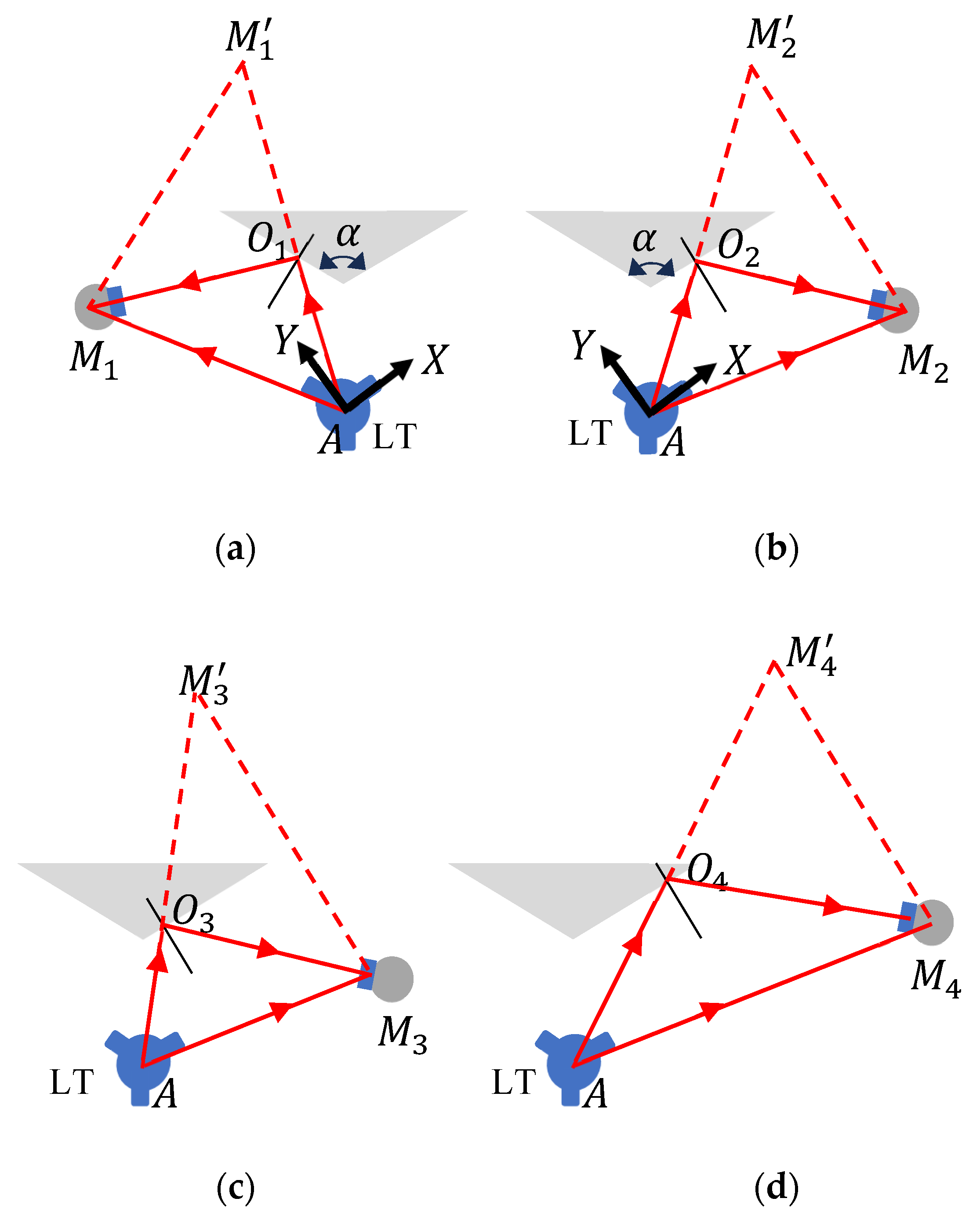
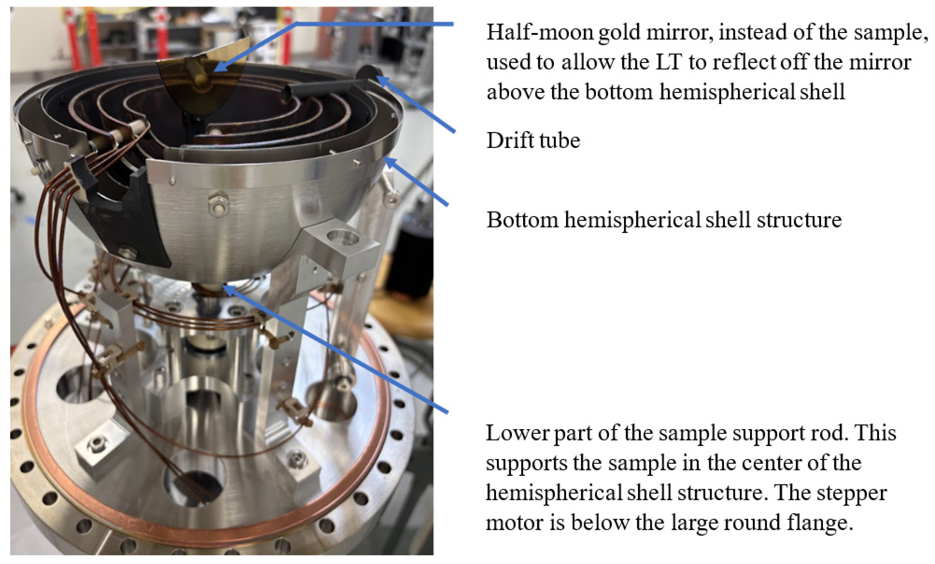
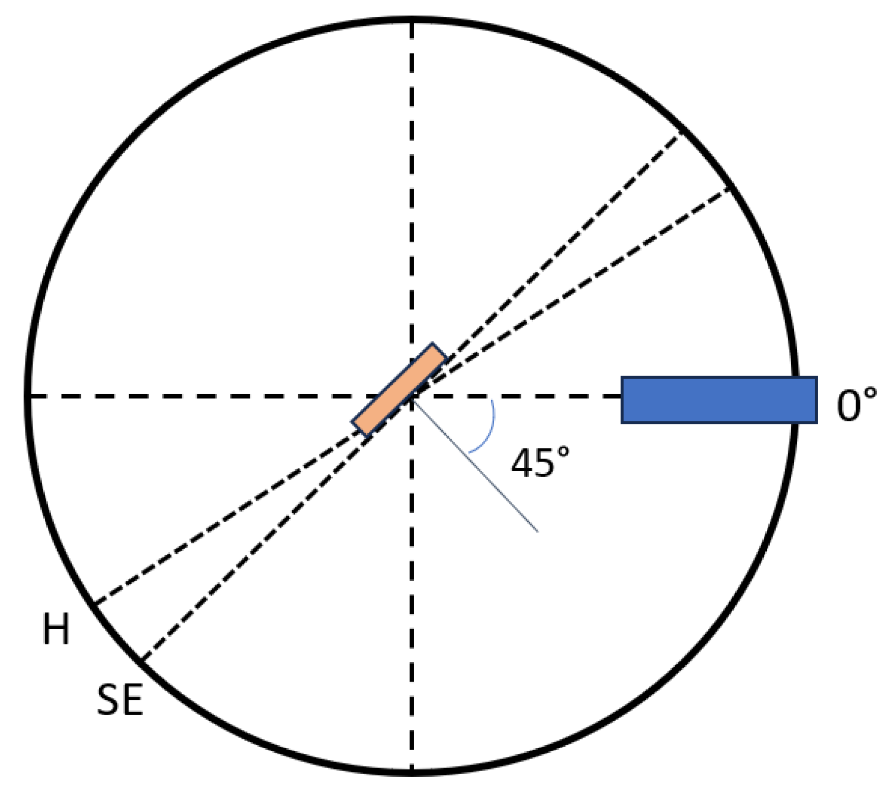
2.2. Mirror-Based Approach
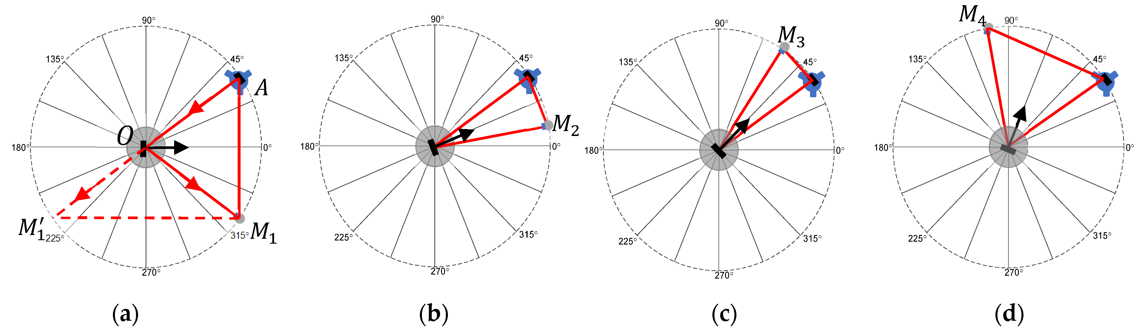
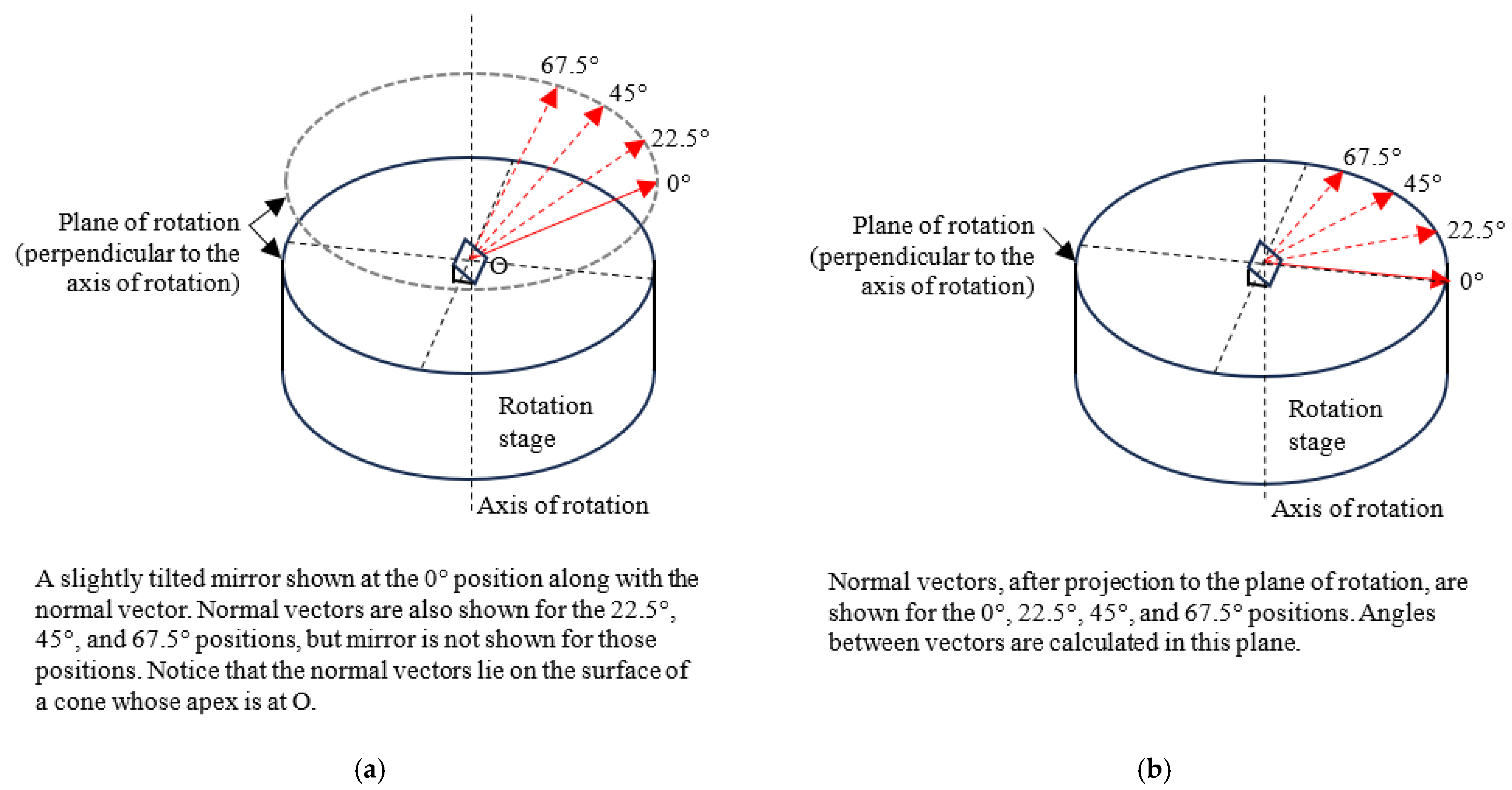
2.2.1. Stitching
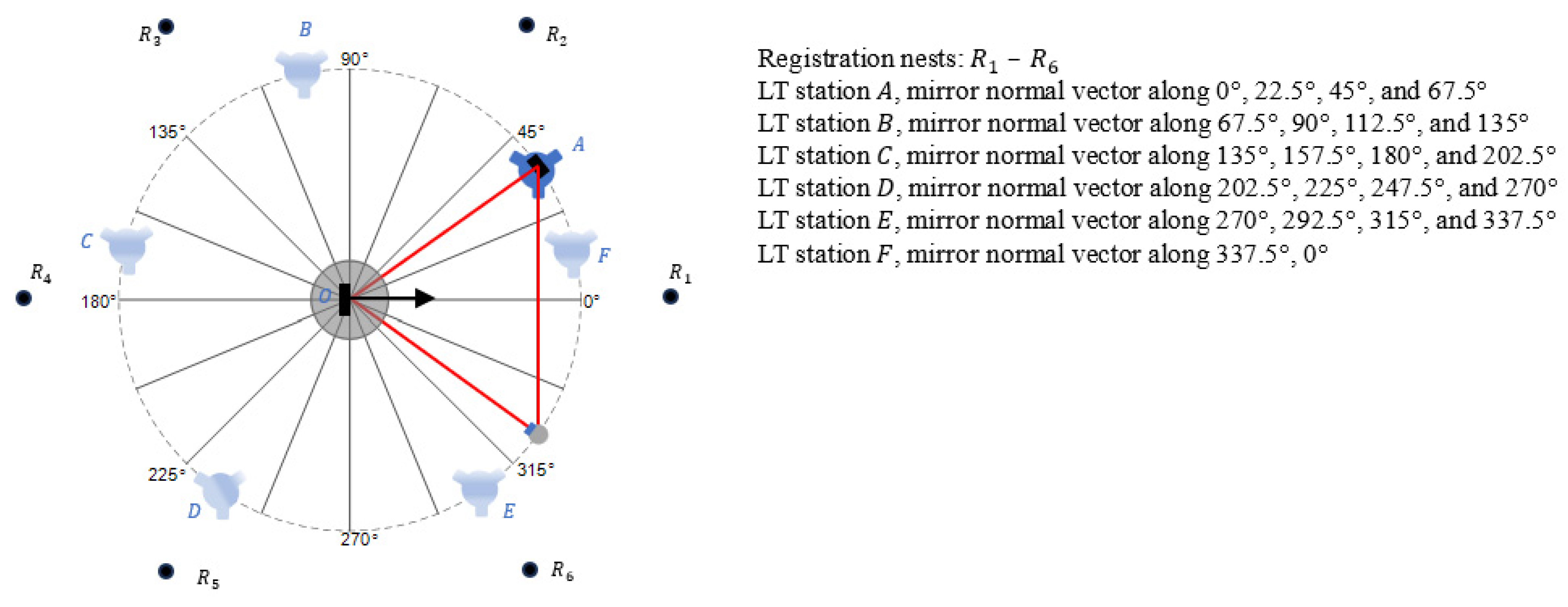
2.2.2. Registration
3. Experiments and Results
3.1. Polygon Measurements
3.2. Precision Spindle Measurements
3.2.1. Verification of Spindle Performance
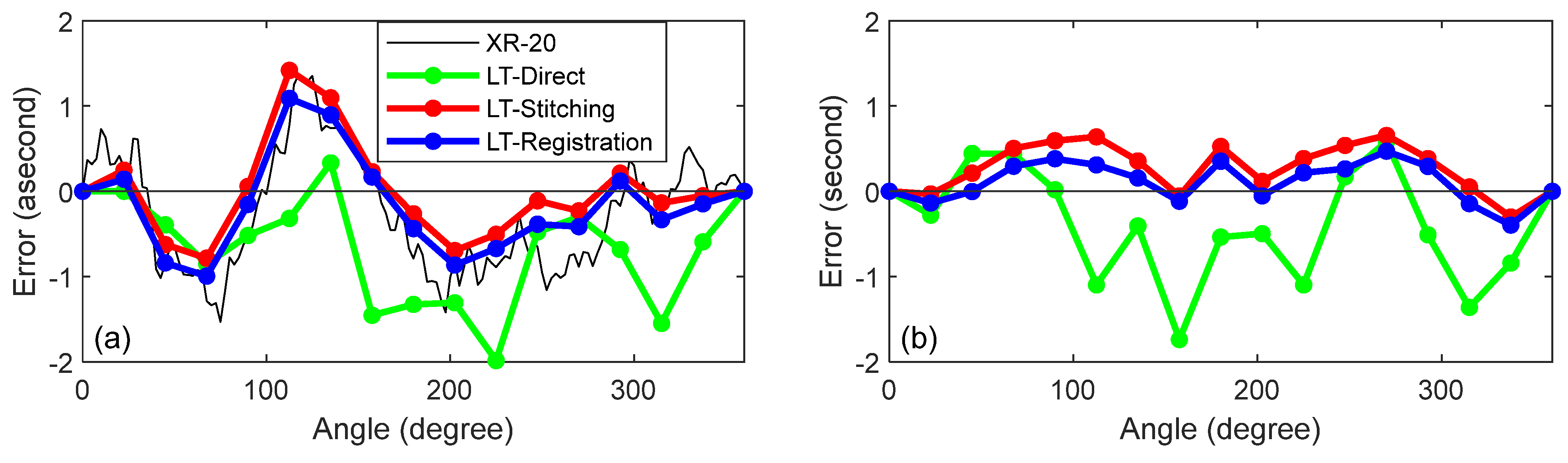
3.2.2. Direct and Mirror-Based Approaches
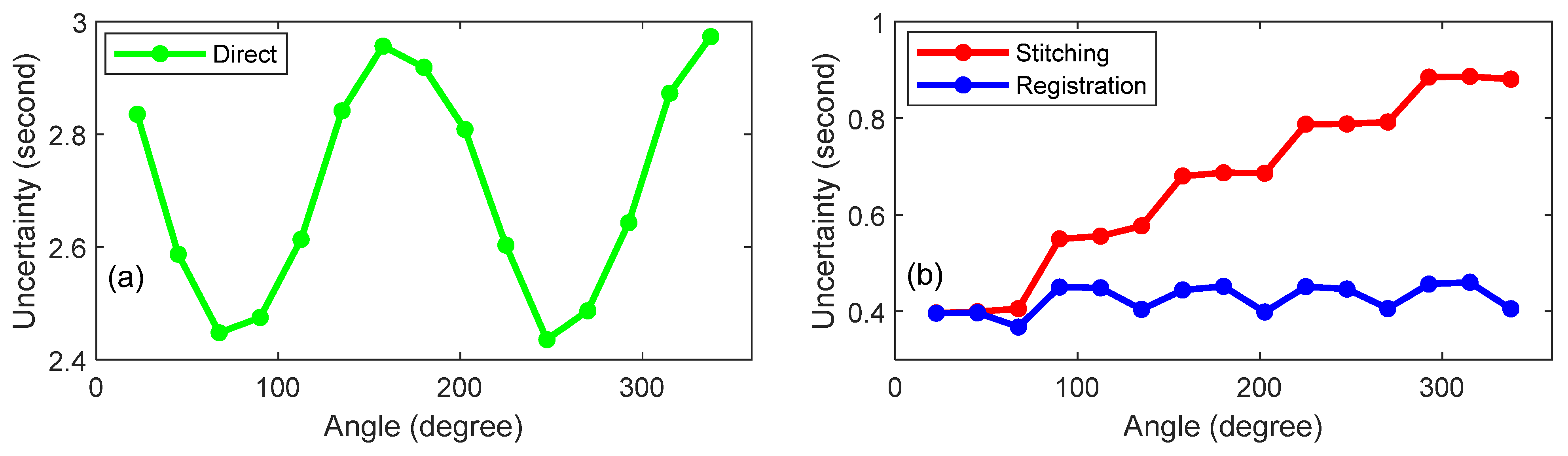
4. Uncertainty and Sensitivity
5. Discussion
6. Conclusions
Author Contributions
Funding
Institutional Review Board Statement
Informed Consent Statement
Data Availability Statement
Acknowledgments
Conflicts of Interest
References
- ASME B89.3.4-2010; Axes of rotation: Methods for Specifying and Testing. The American Society of Mechanical Engineers: New York, NY, USA, 2010.
- ISO 230-7:2015; Test Code for Machine Tools-Part 7: Geometric Accuracy of Axes of Rotation. International Organization for Standardization: Geneva, Switzerland, 2015.
- Marsh, E. Precision Spindle Metrology; Destech Pubns Inc.: Lancaster, PA, USA, 2007. [Google Scholar]
- Chrzanowski, J.; Sałaciński, T.; Skiba, P. Spindle error movements and their measurement. Appl. Sci. 2021, 11, 4571. [Google Scholar] [CrossRef]
- Wang, S.; Ma, R.; Cao, F.; Luo, L.; Li, X. A review: High-precision angle measurement technologies. Sensors 2024, 24, 1755. [Google Scholar] [CrossRef] [PubMed]
- Kumar, A.S.A.; George, B.; Mukhopadhyay, S.C. Technologies and applications of angle sensors: A Review. IEEE Sens. J. 2021, 21, 7195–7206. [Google Scholar] [CrossRef]
- Kinnane, M.N.; Hudson, L.T.; Henins, A.; Mendenhall, M.H. A simple method for high-precision calibration of long-range errors in an angle encoder using an electronic nulling autocollimator. Metrologia 2015, 52, 244–250. [Google Scholar] [CrossRef]
- Jia, H.K.; Yu, L.D.; Zhao, H.N.; Jiang, Y.-Z. A new method of angle measurement error analysis of rotary encoders. Appl. Sci. 2019, 9, 3415. [Google Scholar] [CrossRef]
- Lou, Z.F.; Xue, P.F.; Zheng, Y.S.; Fan, K.C. An analysis of angular indexing error of a gear measuring machine. Appl. Sci. 2018, 8, 169. [Google Scholar] [CrossRef]
- Kin, J.-A.; Lee, J.Y.; Kang, C.-S.; Woo, J.H. High precision vertical angle measurement system for calibration of various angle sensors and instruments. Meas. Sci. Technol. 2024, 35, 075011. [Google Scholar] [CrossRef]
- Hsieh, T.-H.; Watanabe, T.; Hsu, P.-E. Calibration of rotary encoders using a shift-angle method. Appl. Sci. 2022, 12, 5008. [Google Scholar] [CrossRef]
- Mendenhall, M.H.; Henins, A.; Windover, D.; Cline, J.P. Characterization of a self-calibrating, high-precision, stacked-stage, vertical dual-axis goniometer. Metrologia 2016, 53, 933–944. [Google Scholar] [CrossRef]
- Chapma, M.A.V.; Holloway, A.; Lee, W.; May, M.; McFadden, S.; Wall, D. Interferometric Calibration of Rotary Axes. Renishaw Technical White Paper: TE327. Available online: https://www.renishaw.com/resourcecentre/en/details/white-paper-interferometric-calibration-of-rotary-axes--48155 (accessed on 6 March 2025).
- Bao, C.; Feng, Q.; Li, J. Simultaneous measurement method and error analysis of the six degrees-of-freedom motion errors of a rotary axis. Appl. Sci. 2018, 8, 2232. [Google Scholar] [CrossRef]
- Jywe, W.; Chen, C.J.; Hsieh, W.H.; Lin, P.D.; Jwo, H.H.; Yang, T.Y. A novel simple and low cost 4 degree of freedom angular indexing calibrating technique for a precision rotation stage. Int. J. Mach. Tools Manuf. 2007, 47, 1978–1987. [Google Scholar] [CrossRef]
- Hu, C.; Zhu, Y.; Hu, J.; Xu, D.; Zhang, M. An on-axis self-calibration approach for precision rotary metrology stages based on an angular artifact plate. Meas. Sci. Technol. 2013, 24, 085007. [Google Scholar] [CrossRef]
- Dong, H.; Fu, Q.; Zhao, X.; Quan, Q.; Zhang, R. Practical rotation angle measurement method by monocular vision. Appl. Opt. 2015, 54, 425–435. [Google Scholar] [CrossRef]
- Wang, Q.; Miller, J.; Von Freyberg, A.; Steffens, N.; Fischer, A.; Goch, G. Error mapping of rotation stages in 4-axis measuring devices using a ball plate artifact. CIRP Ann. 2018, 67, 559–562. [Google Scholar] [CrossRef]
- Kniel, K.; Franke, M.; Härtig, F.; Keller, F.; Stein, M. Detecting 6 DoF geometrical errors of rotation stages. Measurement 2020, 153, 107366. [Google Scholar] [CrossRef]
- Hsieh, T.H.; Lin, M.X.; Yeh, K.T. Measuring parametric and volumetric errors in a four-axis CMM using a hole plate. Int. J. Precis. Eng. Manuf. 2024, 25, 959–979. [Google Scholar] [CrossRef]
- Chen, J.; Lin, S.; He, B. Geometric error measurement and identification for rotation stage of multi-axis machine tool using double ballbar. Int. J. Mach. Tools Manuf. 2014, 77, 47–55. [Google Scholar] [CrossRef]
- Ibaraki, S.; Iritani, T.; Matsushita, T. Error calibration on five-axis machine tools by on-the-machine measurement of artifacts using a touch-trigger probe. In Proceedings of the 4th CIRP International Conference on High Performance Cutting, Gifu, Japan, 24–26 October 2010. [Google Scholar]
- Wang, J.; Guo, J.; Zhang, G.; Guo, B.; Wang, H. The technical method of geometric error measurement for multi-axis NC machine tool by laser tracker. Meas. Sci. Technol. 2012, 23, 045003. [Google Scholar] [CrossRef]
- Chen, H.; Jiang, B.; Zhang, S.; Shi, Z.; Song, H.; Sun, Y. Calibration method for angular positioning deviation of a high precision rotation stage based on the laser tracer multi-position measurement system. Appl. Sci. 2019, 9, 3417. [Google Scholar] [CrossRef]
- Zha, J.; Li, L.; Chen, Y. Four-station laser tracer-based geometric error measurement of rotation stage. Meas. Sci. Technol. 2020, 31, 065008. [Google Scholar] [CrossRef]
- Hsu, C.-H.; Chen, J.-R.; Hsu, F.-H.; Chen, Y.-T. A novel measurement method for determining geometric errors of rotation stages by using laserTRACER and reflectors. Appl. Sci. 2023, 13, 2419. [Google Scholar] [CrossRef]
- Zhenjiu, Z.; Mingjun, R.; Mingjun, L. A modified sequential multilateration scheme and its application in geometric error measurement of rotary axis. Procedia CIRP 2015, 27, 313–317. [Google Scholar] [CrossRef]
- Ibaraki, S.; Usui, R. A novel error mapping of bi-directional angular positioning deviation of rotary axes in a SCARA-type robot by “open-loop” tracking interferometer measurement. Precis. Eng. 2022, 74, 60–68. [Google Scholar] [CrossRef]
- Ridzel, O.Y.; Yamane, W.; Mansaray, I.; Villarrubia, J.S. Model validation for scanning electron microscopy. In Proceedings of the SPIE 12496, Metrology, Inspection, and Process Control XXXVII, San Jose, CA, USA, 26 February–2 March 2023. [Google Scholar] [CrossRef]
- Villarrubia, J.S.; Vladár, A.E.; Ming, B.; Kline, R.J.; Sunday, D.F.; Chawla, J.S.; List, S. Scanning electron microscope measurement of width and shape of 10nm patterned lines using a JMONSEL-modeled library. Ultramicroscopy 2015, 154, 15–28. [Google Scholar] [CrossRef] [PubMed]
- Wang, L.; Muralikrishnan, B.; Rachakonda, P.; Sawyer, D. Determining geometric error model parameters of a terrestrial laser scanner through two-face, length-consistency, and network methods. Meas. Sci. Technol. 2017, 28, 065016. [Google Scholar] [CrossRef]
- Wang, L.; Muralikrishnan, B.; Lee, V.; Rachakonda, P.; Sawyer, D.; Gleason, J. Methods to calibrate a three-sphere scale bar for laser scanner performance evaluation per the ASTM E3125-17. Measurement 2020, 152, 107274. [Google Scholar] [CrossRef]
- Larichev, R.A.; Filatov, Y.V. A Model of angle measurement using an autocollimator and optical polygon. Photonics 2023, 10, 1359. [Google Scholar] [CrossRef]
- Eves, B.J.; Leroux, I.D. Autocollimators: Plane angle measurand ambiguities and the impact of surface form. Metrologia 2003, 60, 065001. [Google Scholar] [CrossRef]
- Calkins, J.M.; Salerno, R.J. A Practical Method for Evaluating Measurement System Uncertainty; Boeing Large Scale Metrology Conference: Long Beach, CA, USA, 2000. [Google Scholar]


| Method | Uncertainty, U (k = 2) | Observed Error Range | |
|---|---|---|---|
| (Depends on Angle) | Minimum | Maximum | |
| Direct | 2.4 to 3 | −1.7 | +0.6 |
| Mirror Stitching | 0.4 to 0.9 | −0.3 | +0.7 |
| Mirror Registration | 0.4 to 0.5 | −0.4 | +0.5 |
Disclaimer/Publisher’s Note: The statements, opinions and data contained in all publications are solely those of the individual author(s) and contributor(s) and not of MDPI and/or the editor(s). MDPI and/or the editor(s) disclaim responsibility for any injury to people or property resulting from any ideas, methods, instructions or products referred to in the content. |
© 2025 by the authors. Licensee MDPI, Basel, Switzerland. This article is an open access article distributed under the terms and conditions of the Creative Commons Attribution (CC BY) license (https://creativecommons.org/licenses/by/4.0/).
Share and Cite
Muralikrishnan, B.; Shilling, M.; Lee, V.; Ridzel, O.; Holland, G.; Villarrubia, J. A Method to Calibrate Angular Positioning Errors Using a Laser Tracker and a Plane Mirror. Sensors 2025, 25, 1834. https://doi.org/10.3390/s25061834
Muralikrishnan B, Shilling M, Lee V, Ridzel O, Holland G, Villarrubia J. A Method to Calibrate Angular Positioning Errors Using a Laser Tracker and a Plane Mirror. Sensors. 2025; 25(6):1834. https://doi.org/10.3390/s25061834
Chicago/Turabian StyleMuralikrishnan, Bala, Meghan Shilling, Vincent Lee, Olga Ridzel, Glenn Holland, and John Villarrubia. 2025. "A Method to Calibrate Angular Positioning Errors Using a Laser Tracker and a Plane Mirror" Sensors 25, no. 6: 1834. https://doi.org/10.3390/s25061834
APA StyleMuralikrishnan, B., Shilling, M., Lee, V., Ridzel, O., Holland, G., & Villarrubia, J. (2025). A Method to Calibrate Angular Positioning Errors Using a Laser Tracker and a Plane Mirror. Sensors, 25(6), 1834. https://doi.org/10.3390/s25061834