Article

Evaluation of Deadwood Characteristics and Carbon Storage under Different Silvicultural Treatments in a Mixed Broadleaves Mountain Forest

by
Farzam Tavankar
1,
Aezam Rezaee Kivi
2,
Kambiz Taheri-Abkenari
3,
Angela Lo Monaco
4,*,
Rachele Venanzi
4 and
Rodolfo Picchio
4
1
Department of Forestry, Khalkhal Branch, Islamic Azad University, Khalkhal 56817-31367, Iran
2
Department of Plant Biology, Khalkhal Branch, Islamic Azad University, Khalkhal 56817-31367, Iran
3
Department of Forestry, Faculty of Natural Resources, University of Guilan, Somehsara 96196-43619, Iran
4
Department of Agricultural and Forest Sciences, Tuscia University, 01100 Viterbo, Italy
*
Author to whom correspondence should be addressed.
Forests 2022, 13(2), 259; https://doi.org/10.3390/f13020259
Submission received: 13 December 2021 / Revised: 28 January 2022 / Accepted: 1 February 2022 / Published: 7 February 2022
(This article belongs to the Section Wood Science and Forest Products)

Abstract

:
The deadwood (DW) of the forest is in the following two forms: standing (snag) and fallen (log). The DW categories and decay stage are important functional and structural components of forest ecosystems. We used a field-based assessment to quantify how the relative contribution of deadwood to total above-ground carbon stock changes across a silvicultural method and stand altitude gradient in mixed broadleaves stands. The characteristics of DW and carbon stock in selection-cutting managed stands (Sc), shelter-wood managed stands (Sh) and protected stands (Pr) were examined in three altitude ranges (low, <600; medium, 600–1200; and high, >1200 m a.s.l.) in a mixed broadleaves high forest. The results showed that with increasing altitude, the volume of DW increased. The volume of DW in Pr stands was about three times higher than Sh stands and twice higher than Sc stands. The volume of the standing DW was greater than that of the fallen DW in all stands. The highest volume ratio of fallen DW to standing DW was found in the medium altitude in the Sc stand. The amount of carbon stock by DW in the Sh, Sc, and Pr stands was 1.53–2.22, 2.29–3.19, and 5.03–6.80 t ha−1, respectively. The DW share of C-stock of above ground biomass was 4%–4.6% in Sh stand, 4.3%–4.8% in Sc stand, and 7.4%–7.9% in the Pr stand. Deadwood assessment and management, in terms of volume, type, species composition, diameter distribution, spatial allocation and decay stage, is one of the new challenges for a proper sustainable forest management.

1. Introduction

The deadwood (DW) of a forest includes standing dead trees, snags, fallen logs, branches and stumps [1,2]. The DW has an extensive ecological role during and throughout the decomposition stages in forests. These are as follows: sustaining biodiversity [3,4], providing a wide range of habitats for saprotrophic and heterotrophic organisms [5], regulation of nutrient cycling [6,7], regulation of hydrologic processes [8], as well as the provision of habitat for a wide diversity of organisms [9,10], including tree seedlings [11,12]. DW provides a habitat for wildlife such as wood-feeding termites [13,14], cavity-nesting birds [15,16], saproxylic beetles [17] and bats [18]. It facilitates tree regeneration by providing ‘nurse logs’ [19].
One of the most important environmental problems of the present age is global warming due to greenhouse gas emissions [20]. One of the most effective greenhouse gases in global warming is carbon dioxide (CO2) [21]. Green plants capture atmospheric CO2 by storing it in the biomass through photosynthesis [21], reducing the accumulation of CO2 in the atmosphere [22]. Forests play a major role in the carbon cycle and constitute a significant part of the world’s carbon stocks. Forests provide a critical ecosystem service such as carbon repositories, storing more than half of the total carbon stocks in terrestrial ecosystems [23,24,25]. Based on the United Nations Framework Convention on Climate Change (UNFCCC) and the Kyoto Protocol, IPCC Guidelines for National Greenhouse Gas Inventories were established. Forest carbon stock assessment is critical for climate change mitigation measures.
Carbon stocks assessment can globally address climate change mitigation efforts [26]. In this regard, soil carbon dynamic is fundamental to understand nutrient cycling in order to assess the timing of degradation [27,28]. The amount of deadwood biomass is continuously changing in forest ecosystems. These changes depend on the productivity of forest ecosystems, mortality caused by succession processes and disturbances [29], and the decomposition rate [29]. In addition to the geographic region, forest structure and stand composition, forest management methods can also affect the amount and dynamics of DW and the rate of its decomposition in forest ecosystems [16,30,31]. The management regime models applied, as well as the disturbance, affect the quantity and characteristics of dead wood [4] and, to some extent, the stand age [32].
Volume, spatial distribution and characteristics of dead wood in forests, such as dimensions and degree of decay, also depend on the timber harvest [16,33], logging system used [34], level of mechanization [35], density and pattern of forest roads [36], stand distance from adjacent villages [37], human accessibility level [2,33], fuel wood market [38], the presence of pests and diseases [39,40], and succession level of forest stand [41].
Ecologists and forest managers aim to quantify the total biomass or woody carbon per unit area of forests or woodlands [21,42]. Carbon stored in the deadwood of a forest stand is one of the five carbon pools identified by the Intergovernmental Panel on Climate Change that should be measured and monitored for carbon book-keeping [43]. Yet, there is not much study on the relative contribution of DW to carbon stocks in the Hyrcanian forests. The Hyrcanian Forest, a World Heritage site, ranges from Talish in the Republic of Azerbaijan to the Golestan province in Iran. This Forest is located along the northern slopes of the Alborz Mountains to the south of the Caspian Sea. This important forest area is known as a refuge for many ArctoTertiary relicts, which have been classified as Hyrcanian and Euxino-Hyrcanian elements [44,45]. The Iranian Hyrcanian forests in the south of the Caspian Sea, with an area of about 2 million hectares, are recognized as one of the oldest deciduous forests in the world. It has high production capacity due to humid temperate climate and suitable soil. These forests with standing volume of about 300 to 400 m3 and a growth of 5 to 7 m3 per hectare per year, in addition to ecological and economic values, have a high carbon uptake potential. Extensive logging and clearing of forests for agriculture have nearly eliminated the forests in this ecoregion [46].
The Hyrcanian (Caspian) forests with an area of 2 million ha are located between −20 and 2200 m a.s.l. in the north of Iran (south of the Caspian Sea). The Hyrcanian forests encompass various forest types including 80 woody species (trees and shrubs). They are suitable habitats for a variety of hardwood species. The natural dense stands are found at 1000–2100 m and the best stands at 900–1500 m a.s.l. [47].
Many carbon stock studies have either focused exclusively on live standing biomass or have been carried out in primary forests that are unaffected by logging, despite the fact that DW can contain significant portions of the forest carbon stock in the Hyrcanian forests. In this context, the main objectives of this study were to investigate the effect of two different methods of forest management (selection cutting and shelter wood system) on characteristics and amount DW and carbon stored in DW, at different altitudes in mixed deciduous Hyrcanian mountain forests in Iran. To meet these objectives, differences in the volume, distribution, and quality of DW in stands with active management (models of selection cutting and shelter wood system) and conservative management were investigated at three altitude thresholds.
The comparison with protected forests provides interesting insights into the management systems of mixed broad-leaved forests, not only in regard of the amount of deadwood in the different categories and stages of decomposition, but also in relation to the dynamics of deadwood.

2. Materials and Methods

2.1. Study Area

This research was conducted in the Hyrcanian forests in northern Iran (Figure 1). They are natural mixed broadleaves forests. These forests extend from the coastal areas of the Caspian Sea to altitudes of 2700 m above sea level (a.s.l.). Hyrcanian forests are natural and have an uneven structure. In many areas of these forests, shelterwood management has been implemented from 1970 to 2000, and in some areas, only the selection cutting method has been implemented from 2000 onwards. In the study area, harvesting intensity at the last cutting operation in the shelterwood stands was 8.1% to 9.7% of the standing volume, and in the selective logged stands was 5.1% to 12.3% of the standing volume (Table 1). Cut-to-length method using semi-mechanized operation was used, as a dominant harvesting method in the Hyrcanian forests. In the managed areas, by both shelterwood and selection cutting methods, cutting operations were performed by chainsaw and the extraction of logs was performed with rubber wheel skidders.
They were originally managed as shelter wood (Sh) silviculture method, but since 2000, unmanaged stands have been managed by the selection cutting (Sc) silviculture method. In order to investigate the effect of the management method on the volume of DW and the amount of carbon stored in DW, the Nav watershed was selected as a study area, which included stands that were managed by both silvicultural methods and also protected stands (Pr) as control. The Nav watershed is located between 37°38′ to 37°42′ N and 48°48′ to 48°52′ E. Then, the whole surface of the watershed was divided into the following three altitude range classes: low (<600 m a.s.l.), middle (600–1200 m a.s.l.), and high (>1200 m a.s.l.). The choice of thresholds is based on the change of the forest typology with the increase in the altitude.
Two plots with an area of 10 hectares (200 m × 500 m) for each management method and two control plots were selected in each altitude class. In fact, in each altitude class, 6 plots (2 Sh, 2 Sc, and 2 Pr) and 18 plots in the whole study area were randomly selected. The study area has a temperate climate. According to the data of the nearest climatological station, and isothermal and isohyetal maps of Nav Forest watershed, the average annual temperature in the lower, middle and upper stands is 14.1, 12.5 and 9.6 °C, respectively, and the average annual rainfall is 1150, 1360 and 1420 mm, respectively. The forest soil is brown forest type and texture varies from loam clay to loam with good drainage.

2.2. Data Collection

Forest DW mainly includes fallen wood (or logs), snags, and large branches. In addition, stumps above the ground and roots under the ground are also involved because their biomass is almost >20% of those in the whole deadwood, and they play an important role in improving soil structure, maintaining nutrient cycling of the forest, and providing living space for soil organisms [48]. In this study, the volume of DW was estimated in the following two components: standing (standing dead tree and snag) and fallen (log and stump). The stumps (defined as cut tree remains or snags whose trunks are naturally broken at a height of less than 0.5 m) were considered in the fallen DW category due to their low height. In general, stumps are classified as fallen DW or lying deadwood [49]. Estimation of volume per hectare of live trees, snags, fallen logs, and stumps was performed by the methods described as follows.

2.2.1. Volume of Live Trees, Snags, and Stumps

The systematic microplot sampling method was used to estimate the volume of live trees and snags. The grid was positioned at a north–south direction with a random starting point. The dimensions of the network were 100 m by 100 m, the shape of the microplots was circular (R = 17.85 m), and the area of each microplot was 1000 m2. The intersection of the grid dimensions was considered as the center of each microplot. The diameter at breast height (DBH) and height of all living trees and snag species (DBH ≥ 10 cm) were measured in each microplate. The trees and snags DBH was measured by forest caliper (±1 cm accuracy) and the height was assessed by clinometer (±0.1 m). With these parameters, via a local tree volume table, it was possible to estimate the woody volume. The volume of stumps and snags with a height of less than 4 m (short snag) was calculated using Huber’s formula as Equation (1):
V = d m 2 4 × π L
where V is volume (m3), dm is diameter under bark at the middle of stump or short snag (m), and L is height of stump or short snag (m).

2.2.2. Volume of Fallen Logs

The line intersect sampling method was used to estimate the volume of fallen DW. The length of each sample line was 50 m, and the starting point was the center of the same microplots used for the volume estimation of live trees, snags, and stumps. The line transects were oriented on a north–south and east–west direction, totaling to four transects starting from every plot center. The fallen logs intersected by the line transects were measured, considering valid the pieces which were at least 10 cm in diameter under the bark and 30 cm long. For each log the diameter was measured at the point of intersection with a transect line. The volume and weight of these logs in each line transect was computed by Equations (2) and (3), respectively [50]:
V j = π 2 8 L × j = 1 n i d i j 2
W j = S π 2 8 L × j = 1 n i d i j 2
where Vj is volume (m3 ha−1) in line transect j, L is length of line transect (50 m), dij is diameter (cm) of piece i in line transect j, n is number of pieces intersected in line transect j, Wj is weight (t ha−1) in line transect j, S is wood density of pieces. The number of pieces was computed by Equation (4) [50]:
N i = π n i / 2 L l j
where Ni is number of pieces per hectare in diameter class i, ni is number of tallied intersections in diameter class I, L is length of sample line and li is midpoint of diameter class i.

2.2.3. Decay Assessment

For each deadwood element (downed log, snag, and stump) species and decay class were also recorded.
Even if the botanical species of the DW was not always possible to identify, when possible, it was assessed from the bark and macroscopic wood characteristics. The amount of bark on the DW elements was visually valued. The decay class of each deadwood element was determined by the method described by Corace et al. [51] and summarized in Table 2, derived from [2].

2.3. Data Analysis

2.3.1. DW Dynamic Analysis

In order to analyze the dynamics of DW, the following four indices were used [52,53]:
-
Snag creation index (SCI)
S C I = S D W L T
-
Fallen log creation index (FLCI)
F L C I = F D W S V
-
Snag longevity index (SLI)
S L I = F D W S D W
-
Past management legacy index (PMLI)
P M L I = T D W L T
where SDW is standing DW volume, FDW is fallen DW volume, SV is standing volume (live trees + snags), TDW is total DW volume, and LT is live tree volume.

2.3.2. Calculation of C-Stock

In order to calculate the carbon stored in living trees and DW, their mass was first measured by the basic density of the wood and then multiplied by the carbon conversion factor. To calculate the basic density of wood, cylindrical wood samples (CWS) were collected by a drill with a cylindrical coring. The CWS were taken from different species (6 species that make up more than 90% of the volume of living or DW) and different degrees of decay (live tree + 5 decay classes of DW). Five CWS were taken for each live tree species and for each decay class. Therefore, a total of 180 samples (150 from DW and 30 live trees) were taken (6 species × 6 live and decay classes × 5 replication = 180 samples) in the studied stands. The CWS were taken from a height of 1.30 m of living and dead trees, from the intersected sample lines and fallen logs, and from the middle part of the height of the stumps. The basic density of CWS was measured in the laboratory. The volume of CWS was calculated by the volume of the metal cylinder with which the sample was taken. When this method could not be applied, the volume was assessed by the water-displacement method. Dry mass was determined by the gravimetric method after drying in an oven at a temperature of 103 °C ± 2 °C. Basic density (dry mass/green volume) was calculated for each tree species and each decay class of DW. Carbon fraction for above ground biomass in temperate forests, such as the Hyrcanian forests, reported 0.48 by IPPC [54], so carbon content was calculated by the mass of living trees and DW [54].
The carbon content was estimated for each tree species and decay class of DW. Wood basic density is a key functional trait used to estimate aboveground biomass (AGB) and carbon stocks.

2.3.3. Statistical Analysis

The factorial ANOVA test was used to evaluate the effect of the forest silvicultural method on the mean volume and carbon stored in living tree species and decay classes of DW. Duncan’s test was used to detect significant differences among mean values (α = 0.05). The normality distribution of data and equality of variances were confirmed by the Kolmogorov–Smirnov test and Leven’s test, respectively. The relationship between live tree frequency and snag frequency, and between live tree volume and DW volume were analyzed by the Pearson correlation. All statistical analyses were performed using the SPSS version 19 (Chicago, IL, USA) software.

3. Results

3.1. Basic Density by Decay Class

The results of wood density tests showed that the basic density of live trees was significantly higher than the basic density of DW (Table 3). In addition, with the increasing degree of DW decay, the basic density of wood was significantly reduced.

3.2. Effect of Silvicultural Treatments on Stand Structure, DW Distribution and C-Stock by Altitude

3.2.1. Low Altitude (<600 m a.s.l.)

The results of live tree statistics showed that at an altitude of less than 600 m, six tree species had the highest frequency and standing volume in all three studied stands (Table 4). The forest management method had a significant effect on the frequency and volume of trees. The mean frequency and mean tree volume were significantly higher in the Pr stand than in the Sc stand and were higher in the Sc stand than the Sh stand.
The uneven-age structure was characteristic of the three studied stands, so that with increasing tree DBH, the tree frequency decreased, while the volume increased with increasing DBH (Figure 2). The frequency and volume of trees in the Pr stand were higher than the Sc and Sh stands in all DBH classes. The frequency of trees with DBH less than 70 cm in the Sh stand was higher than their frequency in the Sc stand.
The results showed that the volume of fallen, standing, and total DW in the Pr stand was significantly higher than in the Sc stand, and in the Sc stand it was significantly higher than the Sh stand in all DW decay classes (Table 5).
The frequency of fallen DW decreased by the increasing of the diameter class, while the volume increased by the increasing diameter class (Figure 1). The frequency and volume of fallen DW were higher in Pr stand than in Sc and Sh stands in all DW diameter classes. The DW larger than 70 cm in diameter was not observed in the Sh stands. The volume of very large DW in the Sc and Pr stands were 3.78 and 5.98 m3ha−1, respectively.
The frequency of standing DW, like those of fallen DW, decreased with the increasing diameter class, while the volume of standing DW increased by the increasing of the diameter class (Figure 1). The volume of standing DW in diameters larger than 100 cm in the Sc and Pr stands were 4.05 and 8.98 m3ha−1, respectively.
The results showed that the amount of C-stock in DW in the Pr stand was more than three times that of in the Sh, and more than twice that in the Sc stand (Table 6). The amount of C-stock in all decay classes of DW in the Pr stand was higher than in Sc stand, and in the Sc stand was higher than the Sh stand.

3.2.2. Middle Altitude (between 600 and 1200 m a.s.l.)

Unlike altitudes of less than 600 m, beech, hornbeam and oak trees had the highest frequency and volume in all three forest management methods at altitudes of 600–1200 m (Table 7). The frequency and volume of all tree species in Pr stand were significantly higher than in the Sc stand, and in the Sc stand they were significantly higher than in the Sh stand.
As already observed at altitudes between 600 and 1200 m, the structure of the stands was unevenly aged and tree frequency decreased with increasing diameter class, while tree volume increased with increasing diameter class (Figure 3). Frequency and volume of trees were higher in the Pr stand than in the Sc and Sh stands in all diameter classes.
The volume of fallen, standing, and total DW was significantly higher in the Pr stand than in the Sc stand, and in the Sc stand it was significantly higher than in the Sh stand (Table 8). The volume of fallen, standing, and total DW decreased in all three stands with the increasing degree of decay.
As noted at the altitude below 600 m, the frequency of fallen DW decreased by the increasing diameter class, while the volume increased by the increasing diameter class (Figure 2). Moreover, the frequency and volume of fallen DW were higher in the Pr stand than in the Sc and Sh stands in all DW diameter classes. DW with a diameter of more than 100 cm was not observed in the Sh stands. The volume of very large DW in the Sc and Pr stands was 3.23 and 7.86 m3ha−1, respectively.
Similarly at the altitude below 600 m, the frequency of standing DW, decreased with the increasing diameter class, while the volume of standing DW increased by the increasing diameter class (Figure 2). The volume of standing DW in diameters larger than 100 cm in the Sc and Pr stands were 3.26 and 9.71 m3ha−1, respectively.
The results showed that the amount of C-stock in DW in the Pr stand (5.82 t ha−1) was more than three times that of the Sh stand (1.73 t ha−1), and more than twice that of the Sc stand (2.79 t ha−1) (Table 9). The amount of C-stock in all decay classes of DW was higher in the Pr stand than in the Sc stand, and it was higher in the Sc stand than in the Sh stand.

3.2.3. High Altitude (above 1200 m a.s.l.)

At altitudes above 1200 m, more than 80% of the number of trees and more than 60% of the volume of trees consisted of four species of beech, hornbeam, alder and maple (Table 10). As at lower altitudes, the frequency and volume of all tree species were significantly higher in Pr stand than in the Sc stand, and they were significantly higher in the Sc stand than in the Sh stand.
The characteristics of all the stands in this altitude class (Figure 4) were uneven-aged structure, the decreasing number of trees with the increasing DBH, and the increasing volume of trees with the increasing DBH.
Frequency and volume of trees were higher in the Pr stand than in the Sc and Sh stands in all diameter classes, such as at lower altitudes.
Both the fallen and standing volume of DW in the Pr stand were more than twice that in the Sc stand and more than three times that in the Sh stand (Table 11). The volume of fallen, standing, and total DW decreased in all three stands with the increasing degree of decay, such as at lower altitude classes.
In the three different managed stands, the frequency of Fallen DW decreased by the increasing diameter class, while the volume increased by the increasing diameter class (Table 8). In all diameter classes of DW, the frequency of fallen DW was higher in the Pr stand than the Sc stand, and it was higher in the Sc stand than in the Sh stand (Figure 3). The fallen DW with diameter >100 cm was not observed in the Sh stand, while the volume in the Sc and Pr stands were 3.35 and 9.02 m3 ha−1, respectively.
In all three stands, the highest frequency of standing DW was in the small diameter class, while the highest volume of standing DW were in the largest diameter class, but there was none in the Sh (Figure 3). In all diameter classes, the frequency of standing DW was higher in the Pr stand than in the Sc stand, and it was higher in the Sc stand than in the Sh stand.
In all decay classes, C-stock was higher in Pr stand than in Sc stand, and it was higher in Sc stand than in the Sh stand (Table 12).

3.3. Effect of Altitude, Silvicultural Treatments and Their Interaction on Living Trees, DW and C-Stock

The frequency and volume of the live trees were influenced by the silviculture method, altitude range, and their interaction (Table 12). The same results were shown by factorial ANOVA for fallen DW as well. The silviculture method and the altitude range, but not their interaction (Table 12), influenced frequency and volume of standing DW and total DW.
The C-stock assessment for all the categories studied (Table 13) was always affected by the silviculture method, altitude range, and their interaction.

3.4. DW Dynamic

The estimated DW volume was 8.3–17.9 m3 ha−1 in Sh stands, 10.8–22.4 m3 ha−1 in Sc stands, and 30.4–41.6 m3 ha−1 in Pr stands. The volume of standing DW was greater than the volume of fallen DW in all studied stands (Figure 5).
The volume in class DC1 compared to the total DW volume was greater in the Sh than in the Sc. In the Pr it was the lowest (Figure 6) at each altitude. However, the volume in DC4 and DC5 compared to the total DW volume was greater in the Pr than in the SC. In the Sh it was the lowest, at the different altitudes considered.
The value of all indices was higher in the Pr stand than the other two stands, except for the SLI index, which was higher in the Sc stand than the other two stands (Figure 7).
The results of Pearson’s correlation test indicated that there was a significant positive relationship between the snag frequency and live trees frequency (Figure 8) and between DW volume and live tree volume (Figure 9).

3.5. Proportion of C-Stock in Live Trees and DW in Relation Silvicultural Method and Altitude Classes

The results showed that of the total carbon stored in above ground biomass, 92.1 to 95.7% was in the live trees, 2.4 to 4.7% in the standing DW, and 1.5 to 3.2% in the fallen DW (Figure 10).

4. Discussion

Our results showed that the interaction of both the forest management method and the stand altitude a.s.l. had a significant effect on the frequency and volume of live trees, fallen DW, and C-stock. The forest management method and altitude range affected both the frequency and the volume of standing DW and total DW, but their interaction was not significant. Each of the dependent variables is discussed in detail in the following paragraphs.

4.1. Live Trees

Altitude is an easily measurable indicator, which integrates for a number of environmental factors and thus is often used to measure change within assemblages including structure, composition, and species traits [55] Clarifying how forests vary with altitude can increase our understanding of forests and their responses to climate [56].
Our results revealed that the frequency and volume of live trees was highest in the high elevation (1200–1800 m) stands. The increase in annual rainfall from low to high altitudes can be the reason. It can be also due to the change in the composition of tree species because there is an abundance of beech and maple trees at the higher altitudes. In the forests under study beech and maple trees reach a larger diameter and height than other tree species at altitude above 1200 m. With increasing altitude from 1800 upwards, the diameter and height of trees and the volume of forest stands decrease due to decreasing temperature and increasing wind speed in the study area.
The Hyrcanian forests have been managed by different silvicultural treatments [16,47,57], as follows: shelterwood cutting from 1970 to 2000 (Sh stands), selection cutting from 2000 to 2014, and restricted cutting to damaged and fallen trees from 2016 to the present (Sc stands). The main natural disturbance in the Hyrcanian mountain forests in northern Iran is the wind that blows over and damages some trees every year. No tree felling operations have been carried out in the protected stands (Pr stands) since 1970.
The results of this study showed that the frequency and volume of live trees were significantly lower in the harvested stands (Sh and Sc) than the protected stands (Pr), especially the frequency of large diameter trees. Other studies have also concluded that the frequency and volume of trees in the harvested stands were lower than in the protected stands [16,52,58,59,60,61,62,63].

4.2. Deadwood

Deadwood plays several important ecological roles in forest ecosystems. The results of this study showed that the volume of DW in the stands increased with the increasing altitude of the stands as the attributes of living trees are influenced by the silviculture method, the altitude range and their interaction. Hence, it was found that these are the DW drivers.
The rise of DW amount with altitude can be due to a decrease in temperature, due to the fact that as the temperature decreases, the rate of wood decomposition decreases. Moreover, altitude affects other climatic factors such as rainfall and snowfall. Precipitation changes the moisture content of fallen and standing deadwood differently, further influencing the DW decomposition rate [64]. Snowfall may prevalently induce breakage of crown branches [65] producing fallen DW. In the Hyrcanian forest, Tavankar et al. [66] observed crown damage in the larger diameter trees, particularly in Alnus subcordata at the higher elevations, adding that Fagus orientalis was less affected.
There was also a significant relationship between the frequency of live trees and the frequency of snags, and a significant relationship between the volume of live trees and the volume of DW in the stands. Tavankar et al. [67] found that the presence of snags is influenced by the silvicultural regime in the forest and that the distribution was more uniform in both diameter and decay classes in the fully protected forest. Castagneri et al. [68] reported that deadwood characteristics in the montane mixed forests of the Eastern Italian Alps were influenced by altitude and the time elapsed since the last human intervention, as well as by density of live tree and harvesting, similar to the results observed in this study.
The forest type, the age since the establishment of the reserve, and the volume of live trees had been indicated as having a significant influence on the amount of deadwood and its components [53,68,69]. The results of this study showed that the frequency and volume of DW in the harvested stands (Sh and Sc) were significantly lower than the protected stands (Pr). In fact, the Sh and Sc management had reduced the number and volume of DW as compared to the Pr stand, especially the large sizes of DW. However, it is worth noting that the snag volume is greater than that of the logs in each type of both active and conservative management and altitudinal range.
DW volume in forests is governed on a balance of accretion and depletion factors. Disturbance, self-thinning, and senescence constitute factors driving the accumulation of DW. Decay, harvesting of large trees, as well as the right of the local people to collect deadwood are some of the factors that lower the amount and quality of DW [70,71].
Normally, the DW decay rate is inversely proportional to the size of the piece of wood, this could bring to more stable microclimatic conditions [72] and to facilitate the coexistence of species with different ecological requirements [73]; furthermore, these conditions might favor the presence red-listed species [74,75].
Šenhofa et al. [71] studied deadwood characteristics and C-stock in deadwood in mature and old-growth birch stands, in the Latvian forests, observing that the amount of deadwood for mature stands managed was 43.5 m3 ha−1 only slightly lower than some recently abandoned mature stands (51.3 m3 ha−1), but significantly lower than the average values found in old-growth stands (54.4 m3 ha−1). As reported by Öder et al. [76], analyzing DW patterns along altitudinal gradients of managed and unmanaged deciduous forests in western Romania, the managed forest types displayed an average deadwood volume of 47 m3 ha−1 with lying deadwood accounting for over 70%. About 40% of deadwood elements occurred in the early to intermediate decomposition stage, and the deadwood volume in unmanaged forests was two to three times greater than in managed forests. In protected stands (Pr) the amount of deadwood was three times higher than in actively managed stands (Sh and Sc stands).
Ranius et al. [32] studied modeling and dynamics of DW in spruce stands in central Scandinavia, specifically in the country of Norway. They demonstrated that if the forest is managed according to the Forest Certification Standard, the amount of DW with a diameter larger than 10 cm would be almost three times higher than the amount in today’s managed forests.
Deadwood is a fundamental forest habitat component and highly important for biodiversity conservation [76]. The dynamics of production and decay are just as important. The proposed indices on DW dynamic underlined the relationships between the deadwood and the different characteristics of the stand and allow highlighting the dynamics that also exist among the three different management models. The snag-creation index (SCI), fallen log-creation index (FLCI), and past management legacy index (PMLI) were significantly higher in the Pr stands than in the Sc and Sh stands. SCI generally assumes higher values in forest without or with a low pressure of logging activities [2,52,53] and the greater the frequency and volume of living trees, the greater the frequency and volume of snags. FLCI was affected by the time that elapses from the death of standing trees. The greater this time interval, the greater the observed value, because the decayed snags break naturally and increase the fallen log component. Therefore, this index assumes increasing values as the time from active management or logging increases [52,53]. The past management legacy index indicated the influence of deadwood removal over time. The snag longevity index (SLI) was higher in the Sc stands than the Pr and Sh stands. Actively managed forests show higher SLI values [53]. These results are probably related to the restriction on cutting damaged trees, decreed in 2016 in the Caspian managed forests. However, the indices are in line with previous research findings by Tavankar et al. [52], who observed that the cutting of large diameter trees does not give any opportunity for snags or logs to develop in the Sh and Sc stands in Iran. The main factors affecting snag longevity are tree species, tree size, and decay stage. The presence of deadwood in the form of snags, logs and stumps, the diversity of tree species, the occurrence of different diameter classes, and decay stages [1,77] provide resources and increase the availability of niches for a large number of deadwood-dwelling species [78,79]. The distribution of DW in the decay classes showed differences signed by the management regime. It is evident that the Pr stands, at each altitude, exhibited the larger frequencies of DW by volume in the decay classes 4 and 5. Restoring deadwood habitat is vital to recreate fully functioning forest ecosystems [80].

4.3. C-Stock

Growing concerns about the climatic impacts of increased concentrations of atmospheric greenhouse gases have stimulated discussions about the importance and potential of using forests for carbon (C) sequestration [81]. Different studies have shown that with the increasing decomposition stage there is a significant decrease in wood density [82], which is in accordance with the results of this research. The results of this study indicated that C-stock in live trees and DW increased with the increasing stand altitude.
The highest value of C-stock by live trees was estimated in the Pr stands (58.64–85.09 t ha−1), and the lowest in the Sh stands (34.05–46.04 t ha−1). The value of C-stock in the Sc stands was estimated to be 45.42–67.7 t ha−1. Forest ecosystems are an important C pool, retaining approximately 80% of all terrestrial aboveground C and 40%–47% of soil organic C [83,84]. Results of this study showed the DW share of C-stock of above ground biomass was 4%–4.6% in the Sh stand, 4.3%–4.8% in the Sc stand, and 7.4%–7.9% in the Pr stand. This C is released as decomposition proceeds. The amount of C-stock in tropical forests has been reported to be up to 33% [22,85]. The amount of C-stock in living and deadwood biomass varies widely in different forest ecosystems [86]. Lo Monaco et al. [53] highlighted that the deciduous oak forest in the protected lowland forests of central Italy showed an amount of stand volume (379 m3 ha−1), deadwood volume (161.8 m3 ha−1), and C storage (31.43 t ha−1) higher than pine forests and evergreen forests. The mean deadwood carbon pool in mature, recently unmanaged, and old-growth birch (Betula pendula Roth and Betula pubescens Ehrh.) stands was reported as 5.4, 6.3, and 7.9 t ha−1, respectively [71]. In carbon sequestration studies, deadwood is recognized as an important component for conserving C-stock. For example, in the USA, 14% of the total forest carbon pool is stored in deadwood [87].
In addition to having a wide range of ecological roles in forests, deadwood is considered as an important carbon storage of the world. Understanding where carbon is stored in forest structures is essential for accurately estimating forest carbon stocks [88]. The DW acts as a significant carbon and nutrient reservoir [89].
According to the FAO [90], the world’s forests have stored 662 billion tons of carbon, with 44.5% in biomass, 10.3% in deadwood and litter, and 45.2% in soil. The role of deadwood in ecosystem carbon (C) storage has received increasing attention because climate change could alter terrestrial C balance by reducing C storage in this important detrital pool [91,92]. Nations that have signed the agreements are encouraged to quantify C pools and fluxes in their forests, including the proportion occurring as deadwood, and are urged to reduce the greenhouse gas (GHG) emissions into the atmosphere [29].
The decomposition of deadwood is a key factor in the C cycle [29]. After decomposition and humification, the organic C contained in DW becomes an essential component of forest soils [93], contributing to the forest C cycle [94,95]. As such, it acts as a temporary storage pool for C, and represents by decomposition and burial a long-term input source of organic matter and nutrients to the soil [9,96,97].

5. Conclusions

The characteristics of deadwood were assessed in a mixed broadleaves high forest comparing two different management systems applied with protected area. In order to magnify the importance of the research focusing on a larger area, the analysis was replicated at three different altitude ranges. The results showed that with increasing altitude, the volume of deadwood increased. The volume of deadwood in the Pr stands was about three times higher than the Sh stands and twice higher than the Sc stands. The volume of the standing deadwood was greater than that of the fallen deadwood in all stands. The highest volume ratio of fallen deadwood to standing deadwood was found at the mid-range altitude in the Sc stand. The frequency and volume of snags increased at increasing frequency and volume of live trees. The amount of carbon stock by deadwood in the Sh, Sc, and Pr stands was 1.53–2.22, 2.29–3.19, and 5.03–6.80 t ha−1, respectively. The deadwood share of C-stock of above ground biomass was 4%–4.6% in the Sh stand, 4.3%–4.8% in the Sc stand, and 7.4%–7.9% in the Pr stand.
Deadwood assessment and management, in terms of volume, type, species composition, diameter distribution, spatial allocation, and decay stage, is one of the new challenges for a proper sustainable forest management. Management policies for deadwood are important for conservation and the benefits in terms of environmental sustainability. Forest managers need to monitor the impact of their treatments in order to maintain an optimal ratio between ecological and productivity aspects.
The results of this study showed that both silvicultural methods, which are shelter wood and selection cutting, have significantly reduced the deadwood volume as compared to the protected stands in the studied forests. A greater awareness of the dynamics of deadwood is essential in the management of these forests. In addition to producing high quality timber, it is important to pay attention to the dynamic indicators of deadwood during the management of these forests. It seems that modeling protected stands can be a useful guide for managing deadwood in these forests. Due to the ecological importance of deadwood in forests and its environmental values in terms of the carbon reservoir, strategies to increase the volume of deadwood from different types, species, and degrees of decay are necessary. Leaving thicker, decayed, damaged, and wind-fallen trees in the forest is only one of the sustainable management strategies that can be a recommended practice in these forests.

Author Contributions

Conceptualization, F.T., A.R.K., K.T.-A., A.L.M. and R.P.; data curation, F.T., A.R.K., K.T.-A. and A.L.M.; formal analysis, F.T., A.R.K., A.L.M., R.V. and R.P.; investigation, F.T., A.R.K. and K.T.-A.; methodology, F.T., A.R.K., K.T.-A., A.L.M., R.V. and R.P.; resources, A.L.M. and R.P.; supervision, F.T.; validation, F.T., A.R.K., K.T.-A., A.L.M., R.V. and R.P.; visualization, K.T.-A. and R.V.; writing—original draft, F.T., A.R.K., K.T.-A., A.L.M. and R.P.; Writing—review and editing, F.T., A.L.M., R.V. and R.P. All authors have read and agreed to the published version of the manuscript.
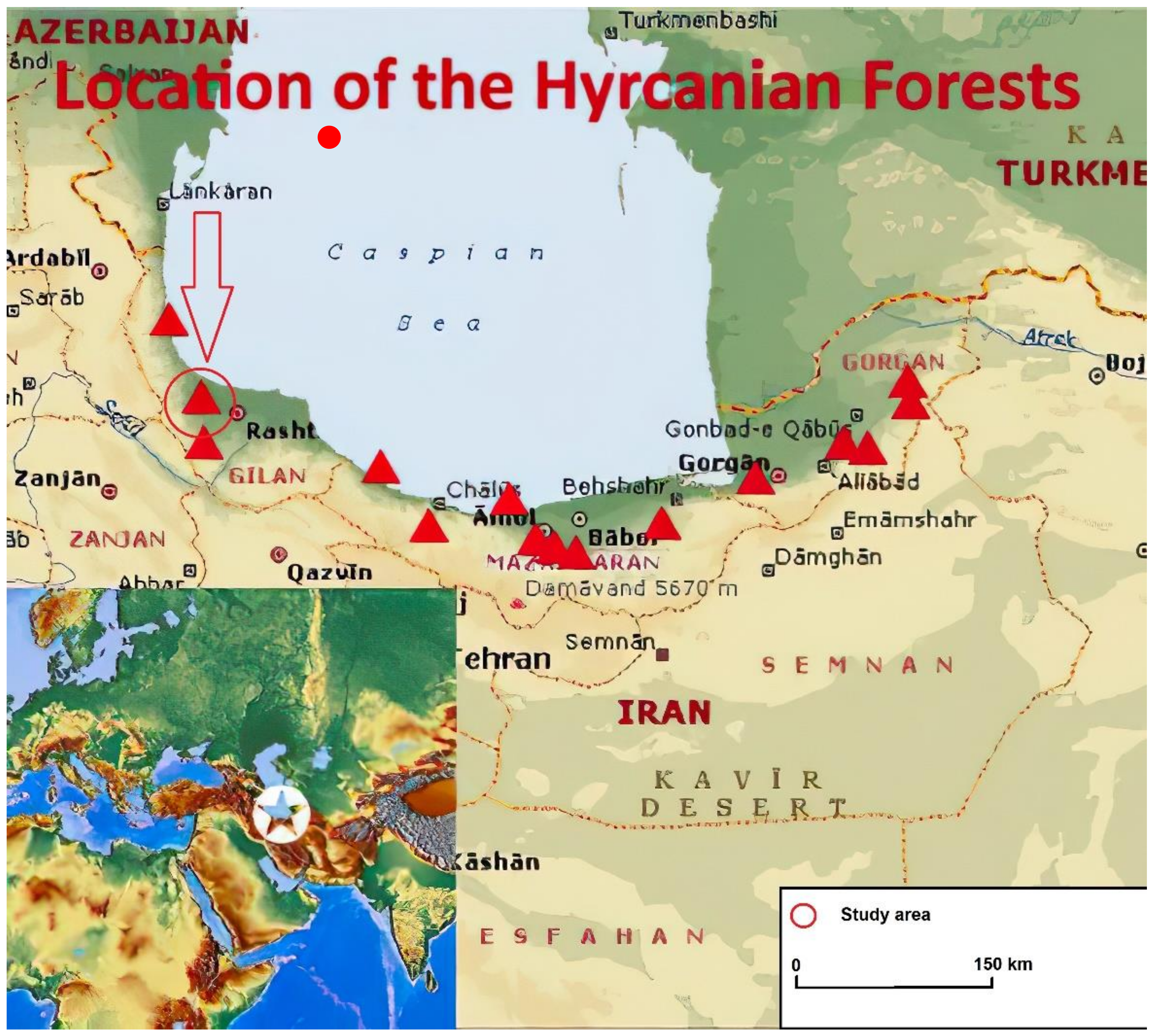
Funding

This research received no external funding.

Institutional Review Board Statement

Not applicable.

Informed Consent Statement

Not applicable.

Data Availability Statement

Data available on request from the corresponding author, due to privacy restrictions.

Acknowledgments

This research was in part carried out within the framework of the MIUR (Italian Ministry for Education, University and Research) initiative “Departments of Excellence” (Law 232/2016), WP 4 (Angela Lo Monaco) WP3 (Rodolfo Picchio), which financed the Department of Agriculture and Forest Science at the University of Tuscia.

Conflicts of Interest

The authors declare no conflict of interest.

References

  1. Kunttu, P.; Junninen, K.; Kouki, J. Dead wood as an indicator of forest naturalness: A comparison of methods. For. Ecol. Manag. 2015, 353, 30–40. [Google Scholar] [CrossRef]
  2. Behjou, F.K.; Lo Monaco, A.; Tavankar, F.; Venanzi, R.; Nikooy, M.; Mederski, P.S.; Picchio, R. Coarse Woody Debris Variability Due to Human Accessibility to Forest. Forests 2018, 9, 509. [Google Scholar] [CrossRef] [Green Version]
  3. Von Oheimb, G.; Westphal, C.; Hardtle, W. Diversity and spatio-temporal dynamics of dead wood in a temperate near-natural beech forest (Fagus sylvatica). Eur. J. For. Res. 2007, 126, 359–370. [Google Scholar] [CrossRef]
  4. Jonsson, B.G.; Ekström, M.; Esseen, P.A.; Grafstrom, A.; Stahl, G.; Westerlund, B. Dead wood availability in managed Swedish forests—Policy outcomes and implications for biodiversity. For. Ecol. Manag. 2016, 376, 174–182. [Google Scholar] [CrossRef] [Green Version]
  5. Jaroszewicz, B.; Cholewinska, O.; Checko, E.; Wrzosek, M. Predictors of diversity of deadwood-dwelling macrofungi in a European natural forest. For. Ecol. Manag. 2021, 490, 119123. [Google Scholar] [CrossRef]
  6. Brais, S.; Pare, D.; Lierman, C. Tree bole mineralization rates of four species of the Canadian eastern boreal forest: Implications for nutrient dynamics following stand-replacing disturbances. Can. J. For. Res. 2006, 36, 2331–2340. [Google Scholar] [CrossRef]
  7. Kuehne, C.; Donath, C.; Muller-Using, S.I.; Bartsch, N. Nutrient fluxes via leaching from coarse woody debris in a Fagus sylvatica forest in the Solling Mountains, Germany. Can. J. For. Res. 2008, 38, 2405–2413. [Google Scholar] [CrossRef]
  8. Lindenmayer, D.B.; Noss, R.E. Salvage logging, ecosystem processes, and biodiversity conservation. Cons. Biol. 2006, 20, 949–958. [Google Scholar] [CrossRef]
  9. Harmon, M.E.; Franklin, J.F.; Swanson, F.J.; Sollins, P.; Gregory, S.V.; Lattin, J.D.; Anderson, N.H.; Cline, S.P.; Aumen, N.G.; Sedell, J.R.; et al. Ecology of coarse woody debris in temperate ecosystems. Adv. Ecol. Res. 1986, 15, 133–302. [Google Scholar]
  10. Lutz, J.A.; Struckman, S.; Furniss, T.J.; Birch, J.D.; Yocom, L.L.; McAvoy, D.J. Large-diameter trees, snags, and deadwood in southern Utah, USA. Ecol. Process. 2021, 10, 9. [Google Scholar] [CrossRef]
  11. Gray, A.N.; Spies, T.A. Microsite controls on tree seedling establishment in conifer forest canopy gaps. Ecology 1997, 78, 2458–2473. [Google Scholar] [CrossRef]
  12. Sanchez, E.; Gallery, R.; Dalling, J.W. Importance of nurse logs as a substrate for the regeneration of pioneer tree species on Barro Colorado Island, Panama. J. Trop. Ecol. 2009, 25, 429–437. [Google Scholar] [CrossRef] [Green Version]
  13. Eggleton, P.; Bignell, D.E.; Sands, W.A.; Waite, B.; Wood, T.G.; Lawton, J.H. The species richness of termites (Isoptera) under differing levels of forest disturbance in the Mbalmayo Forest Reserve, southern Cameroon. J. Tropic. Ecol. 1995, 11, 85–98. [Google Scholar] [CrossRef]
  14. Calderón-Cortés, N.; Escalera-Vázquez, L.H.; Oyama, K. Occurrence of termites (Isoptera) on living and standing dead trees in a tropical dry forest in Mexico. Peer J. 2018, 6, e4731. [Google Scholar] [CrossRef] [PubMed]
  15. Ganey, J.L.; Vojta, S.C. Characteristics of snags containing excavated cavities in northern Arizona mixed-conifer and ponderosa pine forests. For. Ecol. Manag. 2004, 199, 323–332. [Google Scholar] [CrossRef]
  16. Tavankar, F.; Latterini, F.; Nikooy, M.; Venanzi, R.; Naghdi, R.; Picchio, R. Influence of Forest Management and Sylvicultural Treatments on Abundance of Snags and Tree Cavities in Mountain Mixed Beech Forests. Environments 2021, 8, 55. [Google Scholar] [CrossRef]
  17. Grove, S.J. Saproxylic insect ecology and the sustainable management of forests. Annu. Rev. Ecol. Syst. 2002, 33, 1–23. [Google Scholar] [CrossRef]
  18. Giles, E.A. Effects of Tree Cavity Availability on Bat Distribution across a Forest Disturbance Gradient in Sabah, Malaysia. MSc Thesis, University of Kent Canterbury, Canterbury, UK, 2012. [Google Scholar]
  19. Fukasawa, Y. Effects of wood decomposer fungi on tree seedling establishment on coarse woody debris. For. Ecol. Manag. 2012, 266, 232–238. [Google Scholar] [CrossRef]
  20. Mitchard, E.T.A. The tropical forest carbon cycle and climate change. Nature 2018, 559, 527–534. [Google Scholar] [CrossRef]
  21. Khan, M.N.I.; Shil, M.C.; Azad, M.S.; Sadath, M.N.; Feroz, S.; Mollick, A.S. Allometric relationships of stem volume and stand level carbon stocks at varying stand density in Swietenia macrophylla King plantations, Bangladesh. For. Ecol. Manag. 2018, 430, 639–648. [Google Scholar] [CrossRef]
  22. Rice, A.H.; Pyle, E.H.; Saleska, S.R.; Hutyra, L.; Palace, M.; Keller, M.; de Camargo, P.B.; Portilho, K.; Marques, D.F.; Wofsy, S.C. Carbon balance and vegetation dynamics in an old-growth Amazonian forest. Ecol. Appl. 2004, 14, 55–71. [Google Scholar] [CrossRef] [Green Version]
  23. Lewis, S.; Lopez-Gonzalez, G.; Sonké, B.; Affum-Baffoe, K.; Baker, T.R.; Ojo, L.O.; Phillips, O.L.; Reitsma, J.M.; White, L.; Comiskey, J.A.; et al. Increasing carbon storage in intact African tropical forests. Nature 2009, 457, 1003–1006. [Google Scholar] [CrossRef]
  24. Pan, Y.; Birdsey, R.A.; Fang, J.; Houghton, R.; Kauppi, P.E.; Kurz, W.A.; Phillips, O.L.; Shvidenko, A.; Lewis, S.L.; Canadell, J.G.; et al. A large and persistent carbon sink in the world’s forests. Science 2011, 333, 988–993. [Google Scholar] [CrossRef] [Green Version]
  25. Saatchi, S.S.; Harris, N.L.; Brown, S.; Lefsky, M.; Mitchard, E.; Salas, W.; Zutta, B.; Buermann, W.; Lewis, S.; Hagen, S.; et al. Benchmark map of forest carbon stocks in tropical regions across three continents. Proc. Natl. Acad. Sci. USA 2011, 108, 9899–9904. [Google Scholar] [CrossRef] [Green Version]
  26. Brown, S. Measuring carbon in forests: Current status and future challenges. Environ. Pollut. 2002, 116, 363–372. [Google Scholar] [CrossRef]
  27. Fogel, R.; Cromack, K. Effect of habitat and substrate quality on Douglas-fir litter decomposition in Western Oregon. Can. J. Bot. 1977, 55, 1632–1640. [Google Scholar] [CrossRef]
  28. Johansson, M.B.; Berg, B.; Meentemeyer, V. Litter mass-loss rates in late stages of decomposition in a climatic transect of pine forests. Long-term decomposition in a Scots pine forest. IX. Can. J. Bot. 1995, 73, 1509–1521. [Google Scholar] [CrossRef]
  29. Köster, K.; Metslaid, M.; Engelhart, J.; Köster, E. Dead wood basic density, and the concentration of carbon and nitrogen for main tree species in managed hemiboreal forests. For. Ecol. Manag. 2015, 354, 35–42. [Google Scholar] [CrossRef]
  30. Taheri-Abkenari, K.; Akbari, F.; Pilehvar, B. Effect of intervention and type of forest management on quality and quantity characteristics of dead wood in managed and reserve forests: A case study. J. For. Res. 2012, 23, 413–418. [Google Scholar] [CrossRef]
  31. Banaś, J.; Leszek Bujoczek, L.; Stanisław Zięba, S.; Drozd, M. The effects of different types of management, functions, and characteristics of stands in Polish forests on the amount of coarse woody debris. Eur. J. For. Res. 2014, 133, 1095–1107. [Google Scholar] [CrossRef] [Green Version]
  32. Ranius, T.; Kindvall, O.; Kruys, N.; Jonsson, B.G. Modelling dead wood in Norway spruce stands subject to different management regimes. For. Ecol. Manag. 2003, 182, 13–29. [Google Scholar] [CrossRef]
  33. Wisdom, M.J.; Bate, L.J. Snag density varies with intensity of timber harvest and human access. For. Ecol. Manag. 2008, 255, 2085–2093. [Google Scholar] [CrossRef]
  34. Nappi, A.; Drapeau, P.; Savard, J.-P.L. Salvage logging after wildfire in the boreal forest: Is it becoming a hot issue for wildlife? For. Chron. 2004, 80, 67–74. [Google Scholar] [CrossRef]
  35. Titus, B.D.; Brown, K.; Helmisaari, H.-S.; Vanguelova, E.; Stupak, I.; Evans, A.; Clarke, N.; Guidi, C.; Bruckman, V.J.; Varnagiryte-Kabasinskiene, I.; et al. Sustainable forest biomass: A review of current residue harvesting guidelines. Energy Sustain. Soc. 2021, 11, 10. [Google Scholar] [CrossRef]
  36. Akay, M.E.; Serin, H.; Seesions, J.; Bilici, E.; Pak, M. Evaluating the Effects of Improving Forest Road Standards on Economic Value of Forest Products. Croat. J. For. Eng. 2021, 42, 245–258. [Google Scholar] [CrossRef]
  37. Bate, L.J.; Wisdom, M.J.; Wales, B.C. Snag densities in relation to human access and associated management factors in forests of northeastern Oregon, USA. Landsc. Urban Plan. 2007, 80, 278–291. [Google Scholar] [CrossRef]
  38. Stephens, S.L. Fuel loads, snag abundance, and snag recruitment in an unmanaged Jeffrey pine–mixed conifer forest in Northwestern Mexico. For. Ecol. Manag. 2004, 199, 103–113. [Google Scholar] [CrossRef]
  39. Harris, R.B. Abundance and Characteristics of Snags in Western Montana Forests; U.S. Department of Agriculture, Forest Service, Rocky Mountain Research Station: Fort Collins, CO, USA, 1999; p. 19. [Google Scholar]
  40. McCollum, D.W.; Lundquist, J.E. Bark Beetle Infestation of Western US Forests: A Context for Assessing and Evaluating Impacts. J. For. 2019, 117, 171–177. [Google Scholar] [CrossRef]
  41. Sefidi, K. The influence of forest management histories on dead wood and habitat trees in the old growth forest in Northern Iran. Int. J. Biol. Biomol. Agric. Food Biotech. Eng. 2015, 9, 1014–1018. [Google Scholar]
  42. Lo Monaco, A.; Cantiani, P. Forest stand management and biomass growth. Forests 2021, 12, 1253. [Google Scholar] [CrossRef]
  43. Watson, R.T.; Noble, I.R.; Bolin, B.; Ravindranath, N.H.; Verardo, D.J.; Dokken, D.J. Land use, Land-Use Change and Forestry IPPC Report; Cambridge University Press: Cambridge, UK, 2000; Available online: https://www.ipcc.ch/report/land-use-land-use-change-and-forestry/ (accessed on 12 December 2021).
  44. Zohary, M. Geobotanical Foundations of the Middle East; Fischer: Quezon City, Philippines, 1973; p. 738. [Google Scholar]
  45. Alavi, S.J.; Veiskarami, R.; Esmailzadeh, O.; Gadow, K.v. Analyzing the Biological and Structural Diversity of Hyrcanian Forests Dominated by Taxus baccata L. Forests 2020, 11, 701. [Google Scholar] [CrossRef]
  46. Müller, J.; Sagheb-Talebi, K.; Thorn, S. Protect Iran’s ancient forest from logging. Science 2017, 355, 6328. [Google Scholar] [CrossRef]
  47. Talebi, K.S.; Schütz, J.P. The structure of natural oriental beech (Fagus orientalis) forests in the Caspian region of Iran and the potential for the application of the group selection system. Forestry 2002, 75, 465–472. [Google Scholar] [CrossRef] [Green Version]
  48. Currie, W.S.; Jadelhoffer, K.N. The imprint of land use history: Patterns of carbon and nitrogen in downed woody debris at the Harvard forest. Ecosystems 2002, 5, 446–460. [Google Scholar] [CrossRef]
  49. Merganičová, K.; Merganič, J. Coarse woody debris carbon stocks in natural spruce forests of Babia hora. J. For. Sci. 2010, 56, 397–405. [Google Scholar] [CrossRef] [Green Version]
  50. Van Wagner, C.E. Canada Information Report PI-X-12: Practical Aspects of the Line Intersect Method; Petawawa Canadian National Forestry Institute Forestry Service: Chalk River, ON, Canada, 1982. [Google Scholar]
  51. Corace, R.G.; Seefelt, N.E.; Goebel, P.C.; Shaw, H.L. Snag longevity and decay class development in a recent Jack Pine clearcut in Michigan. North J. App. For. 2010, 27, 125–131. [Google Scholar] [CrossRef] [Green Version]
  52. Tavankar, F.; Nikooy, M.; Picchio, R.; Venanzi, R.; Lo Monaco, A. Long-term effects of single-tree selection cutting management on coarse woody debris in natural mixed beech stands in the Caspian forest (Iran). iForest 2017, 10, 652–658. [Google Scholar] [CrossRef] [Green Version]
  53. Lo Monaco, A.; Luziatelli, G.; Latterini, F.; Tavankar, F.; Picchio, R. Structure and Dynamics of Deadwood in Pine and Oak Stands and their Role in CO2 Sequestration in Lowland Forests of Central Italy. Forests 2020, 11, 253. [Google Scholar] [CrossRef] [Green Version]
  54. IPCC, Default Biomass Conversion and Expansion Factors. IPCC Guidelines for National Greenhouse Gas Inventories 2006, Agriculture, Forestry and Other Land Use. In Proceeding of the Intergovernmental Panel on Climate Change 2006; The Institute for Global Environmental Strategies for the IPCC: Tokyo, Japan, 2006.
  55. Hunter, J.T. Changes in Allometric attributes and biomass of forests and woodlands across an altitudinal and rainfall gradient: What are the implications of increasing seasonality due to anthropogenic climate change? Int. J. Ecol. 2015, 2015, 208975. [Google Scholar] [CrossRef]
  56. Mazón, M.M.; Klanderud, K.; Finegan, B.; Veintimilla, D.; Bermeo, B.; Murrieta, E.; Delgado, D.; Sheil, D. How forest structure varies with elevation in old growth and secondary forest in Costa Rica. For. Ecol. Manag. 2020, 469, 118191. [Google Scholar] [CrossRef]
  57. Bodaghi, A.I.; Nikooy, M.; Naghdi, R.; Tavankar, F. Logging damage to residual trees during sustainable harvesting of uneven-age stands in the Hyrcanian forests of Iran. N. Z. J. For. Sci. 2020, 50, 1–11. [Google Scholar] [CrossRef] [Green Version]
  58. McComb, W.C.C.; Rumsey, R.L. Characteristics and Cavity-Nesting Bird Use of Picloram-Created Snags in the Central Appalachians. South J. Appl. For. 1983, 7, 34–37. [Google Scholar] [CrossRef]
  59. Goodburn, J.M.; Lorimer, C.G. Cavity trees and coarse woody debris in old-growth and managed northern hardwood forests in Wisconsin and Michigan. Can. J. For. Res. 1998, 28, 427–438. [Google Scholar] [CrossRef]
  60. McGee, G.G.; Leopold, D.J.; Nyland, R.D. Structural characteristics of old-growth, maturing, and partially cut northern hardwood forests. Ecol. Appl. 1999, 9, 1316–1329. [Google Scholar] [CrossRef]
  61. Verburg, R.; Van Eijk-Bos, C. Effects of selective logging on tree diversity, composition and plant functional type patterns in a Bornean rain forest. J. Veg. Sci. 2003, 14, 99–110. [Google Scholar] [CrossRef]
  62. Bebber, D.P.; Cole, W.G.; Thomas, S.C.; Balsillie, D.; Duinker, P. Effects of retention harvests on structure of old-growth Pinus strobus L. stands in Ontario. For. Ecol. Manag. 2005, 205, 91–103. [Google Scholar] [CrossRef]
  63. Villela, D.M.; Nascimento, M.T.; De Aragao, L.E.O.C.; Gama, D.M. Effect of selective logging on forest structure and nutrient cycling in a seasonally dry Brazilian Atlantic forest. J. Biogeogr. 2006, 33, 505–516. [Google Scholar] [CrossRef]
  64. Dai, Z.; Trettin, C.C.; Burton, A.J.; Jurgensen, M.F.; Page-Dumroese, D.S.; Forschler, B.T.; Schilling, J.S.; Lindner, D.L. Coarse woody debris decomposition assessment tool: Model development and sensitivity analysis. PLoS ONE 2021, 16, e0251893. [Google Scholar] [CrossRef] [PubMed]
  65. Peltola, H.; Nykänen, M.L.; Kelloäki, S. Model computations on the critical combination of snow loading and wind speed for snow damage of Scots pine, Norway spruce and birch sp. at stand edge. For. Ecol. Manag. 1997, 95, 229–241. [Google Scholar] [CrossRef]
  66. Tavankar, F.; Lo Monaco, A.; Nikooy, M.; Venanzi, R.; Bonyad, A.E.; Picchio, R. Snow damages on trees of an uneven age in mixed broadleaf forests: Effects of topographical conditions and tree characteristics. J. For. Res. 2019, 30, 1383–1394. [Google Scholar] [CrossRef]
  67. Tavankar, F.; Picchio, R.; Lo Monaco, A.; Bonyad, A.E. Forest management and snag characteristics in Northern Iran lowland forests. J. For. Sci. 2014, 60, 431–441. [Google Scholar] [CrossRef] [Green Version]
  68. Castagneri, D.; Garbarino, M.; Berretti, R.; Motta, R. Site and stand effects on coarse woody debris in montane mixed forests of Eastern Italian Alps. For. Ecol. Manag. 2010, 260, 1592–1598. [Google Scholar] [CrossRef] [Green Version]
  69. Christensen, M.; Hahn, K.; Mountford, E.P.; Odor, P.; Standovár, T.; Rozenbergar, D.; Diaci, J.; Wijdeven, S.; Meyer, P.; Winter, S. Dead wood in European beech (Fagus sylvatica) forest reserves. For. Ecol. Manag. 2005, 210, 267–282. [Google Scholar] [CrossRef]
  70. Woodall, C.W.; Westfall, J.A. Relationships between the stocking levels of live trees and dead tree attributes in forests of the United States. For. Ecol. Manag. 2009, 258, 2602–2608. [Google Scholar] [CrossRef]
  71. Šenhofa, S.; Jaunslaviete, I.; Šnepsts, G.; Jansons, J.; Liepa, L.; Jansons, A. Deadwood Characteristics in Mature and Old-Growth Birch stands and their implications for carbon storage. Forests 2020, 11, 536. [Google Scholar] [CrossRef]
  72. Parisi, F.; Pioli, S.; Lombardi, F.; Fravolini, G.; Marchetti, M.; Tognetti, R. Linking deadwood traits with saproxylic invertebrates and fungi in European forests-a review. iForest 2018, 11, 423–436. [Google Scholar] [CrossRef] [Green Version]
  73. Heilmann-Clausen, J.; Christensen, M. Does size matter? On the importance of various dead wood fractions for fungal diversity in Danish beech forests. For. Ecol. Manag. 2004, 201, 105–117. [Google Scholar] [CrossRef]
  74. Siitonen, J.; Saaristo, L. Habitat requirements and conservation of Pytho kolwensis, a beetle species of old-growth boreal forest. Biol. Conserv. 2000, 94, 211–220. [Google Scholar] [CrossRef]
  75. Pouska, V.; Svoboda, M.; Lepšová, A. The diversity of wood-decaying fungi in relation to changing site conditions in an old-growth mountain spruce forest, Central Europe. Eur. J. For. Res. 2010, 129, 219–231. [Google Scholar] [CrossRef]
  76. Öder, V.; Petritan, A.M.; Schellenberg, J.; Bergmeier, E.; Walentowski, H. Patterns and drivers of deadwood quantity and variation in mid-latitude deciduous forests. For. Ecol. Manag. 2021, 487, 118977. [Google Scholar] [CrossRef]
  77. Siitonen, J. Forest management, coarse woody debris and saproxylic organisms: Fennoscandian boreal forest as an example. Ecol. Bull. 2001, 49, 11–41. [Google Scholar]
  78. Pretzsch, H. Analysis and modelling of spatial stand structures. Methodological considerations based on mixed beech-larch stands in Lower Saxony. For. Ecol. Manag. 1997, 97, 237–253. [Google Scholar] [CrossRef]
  79. Seibold, S.; Bassler, C.; Brandl, R.; Gossner, M.M.; Thorn, S.; Ulyshen, M.D.; Müller, J. Experimental studies of dead-wood biodiversity—A review identifying global gaps in knowledge. Biol. Cons. 2015, 191, 139–149. [Google Scholar] [CrossRef]
  80. Burns, M.L.; Smith, M.; Slade, E.; Ennos, R.A. The Saproxylic Activity Index: A New Tool for the Rapid Assessment of Deadwood Species during Forest Restoration. Open J. For. 2014, 4, 144–150. [Google Scholar] [CrossRef] [Green Version]
  81. Yeboah, D.; Burton, A.J.; Storer, A.J.; Opuni-Frimpong, E. Variation in wood density and carbon content of tropical plantation tree species from Ghana. New For. 2014, 45, 35–52. [Google Scholar] [CrossRef]
  82. Di Cosmo, L.; Gasparini, P.; Paletto, A.; Nocetti, M. Deadwood basic density values for national-level carbon stock estimates in Italy. For. Ecol. Manag. 2013, 295, 51–58. [Google Scholar] [CrossRef]
  83. Jobbágy, E.G.; Jackson, R.B. The vertical distribution of soil organic carbon and its relation to climate and vegetation. Ecol. Appl. 2000, 10, 423–436. [Google Scholar] [CrossRef]
  84. Wei, X.; Shao, M.; Gale, W.; Li, L. Global pattern of soil carbon losses due to the conversion of forests to agricultural land. Sci. Rep. 2014, 4, 4062. [Google Scholar] [CrossRef] [PubMed]
  85. Clark, D.B.; Clark, D.A.; Brown, S.; Oberbauer, S.F.; Veldkamp, E. Stocks and flows of coarse woody debris across a tropical rain forest nutrient and topography gradient. For. Ecol. Manag. 2002, 164, 237–248. [Google Scholar] [CrossRef]
  86. Shorohova, E.; Kapitsa, E.; Kuznetsov, A.; Kuznetsova, S.; de Gerenuy, V.L.; Kaganov, V.; Kurganova, I. Decay classes of coarse woody debris in a lowland Dipterocarp forest: Implications for volume, density, and carbon estimates. Biotropica 2021, 53, 879–887. [Google Scholar] [CrossRef]
  87. Woodall, C.W.; Liknes, G.C. Climatic regions as an indicator of forest coarse and fine woody debris carbon stocks in the United States. Carbon Balance Manag. 2008, 3. [Google Scholar] [CrossRef] [PubMed] [Green Version]
  88. Jones, G.M.; Keane, J.J.; Gutiérrez, R.J.; Peery, M.Z. Declining old-forest species as a legacy of large trees lost. Divers. Distrib. 2018, 24, 341–351. [Google Scholar] [CrossRef] [Green Version]
  89. Chambers, J.Q.; Higuchi, N.; Schimel, J.P.; Ferreira, L.V.; Melack, J.M. Decomposition and carbon cycling of dead trees in tropical forests of the central Amazon. Oecologia 2000, 122, 380–388. [Google Scholar] [CrossRef] [PubMed]
  90. FAO. Global Forest Resources Assessment 2020; Main Report; FAO: Rome, Italy, 2020. [Google Scholar] [CrossRef]
  91. Weedon, J.T.; Cornwell, W.K.; Cornelissen, J.H.C.; Zanne, A.E.; Wirth, C.; Coomes, D.A. Global meta-analysis of wood decomposition rates: A role for trait variation among tree species? Ecol. Lett. 2009, 12, 45–56. [Google Scholar] [CrossRef]
  92. Iwashita, D.K.; Litton, C.M.; Giardina, C.P. Coarse woody debris carbon storage across a mean annual temperature gradient in tropical montane wet forest. For. Ecol. Manag. 2013, 291, 336–343. [Google Scholar] [CrossRef]
  93. Kahl, T.; Baber, K.; Otto, P.; Wirth, C.; Bauhus, J. Drivers of CO2 emission rates from dead wood logs of 13 tree species in the initial decomposition phase. Forests 2015, 6, 2484–2504. [Google Scholar] [CrossRef] [Green Version]
  94. Laiho, R.; Prescott, C.E. The contribution of coarse woody debris to carbon, nitrogen and phosphorus cycles in three Rocky Mountain coniferous forests. Can. J. For. Res. 1999, 29, 1592–1603. [Google Scholar] [CrossRef]
  95. Janisch, J.E.; Harmon, M.E. Successional changes in live and dead wood carbon stores: Implications for net ecosystem productivity. Tree Physiol. 2002, 22, 77–89. [Google Scholar] [CrossRef] [Green Version]
  96. Goodale, C.L.; Apps, M.J.; Birdsey, R.A.; Field, C.B.; Heath, L.S.; Houghton, R.A.; Jenkins, J.C.; Kohlmaier, G.H.; Kurz, W.; Liu, S.; et al. Forest carbon sinks in the Northern hemisphere. Ecol. Appl. 2002, 12, 891–899. [Google Scholar] [CrossRef]
  97. Moroni, M.T.; Morris, D.M.; Shaw, C.; Stokland, J.N.; Harmon, M.E.; Fenton, N.J.; Merganicová, K.; Merganic, J.; Okabe, K.; Hagemann, U. Buried wood.3390A common yet poorly documented form of deadwood. Ecosystems 2015, 18, 605–628. [Google Scholar] [CrossRef]
Figure 1. Map of Hyrcanian forests, and location of study area (red circle).
Forests 13 00259 g001
Figure 2. The bars show the number of living trees (a), fallen DW (b) and standing DW (c) in altitude of <600 m referred to diameter (DBH) distribution in each silviculture method (left y-axis). The scatter bars show the volume of living trees (a), fallen DW (b) and standing DW (c) per DBH class (right y-axis). Sh, shelter wood silviculture; Sc, selection cutting silviculture; Pr, protected stand.
Forests 13 00259 g002
Figure 3. The bars show the number of living trees (a), fallen DW (b) and standing DW (c) in altitude of 600–1200 m referred to diameter distribution in each silviculture method (left y-axis). The scatter bars show the volume of living trees (a), fallen DW (b) and standing DW (c) per diameter class (right y-axis). Sh, shelter wood silviculture; Sc, selection cutting silviculture; Pr, protected stand.
Forests 13 00259 g003aForests 13 00259 g003b
Figure 4. The bars show the number of living trees (a), fallen DW (b) and standing DW (c) in altitude of >1200 m referred to diameter distribution in each silviculture method (left y-axis). The scatter bars show the volume of living trees (a), fallen DW (b) and standing DW (c) per DBH class (right y-axis). Sh, shelter wood silviculture; Sc, selection cutting silviculture; Pr, protected stand.
Forests 13 00259 g004aForests 13 00259 g004b
Figure 5. Volume proportion of standing and fallen DW in different silvicultural managed stands. Sh, shelter wood silviculture; Sc, selection cutting silviculture; Pr, protected stand.
Forests 13 00259 g005
Figure 6. Volume proportion of each decay classes of DW in different silvicultural managed stands. Sh, shelter wood silviculture; Sc, selection cutting silviculture; Pr, protected stand.
Forests 13 00259 g006
Figure 7. Value of DW indices by altitude class and silvicultural management. Sh, shelter wood silviculture; Sc, selection cutting silviculture; Pr, protected stand. SCI, snag creation index; FLCI, fallen log creation index; SLI, snag longevity index; and PMLI, past management legacy index.
Forests 13 00259 g007
Figure 8. Snag frequency in relation with live tree frequency.
Forests 13 00259 g008
Figure 9. DW volume in relation with live tree volume.
Forests 13 00259 g009
Figure 10. Proportion of C-stock in live trees, fallen and standing DW in different silvicultural managed stands. Sh, shelter wood silviculture; Sc, selection cutting silviculture; Pr, protected stand.
Forests 13 00259 g010
Table 1. Stand and operation characteristics in the study area (Sh, shelter wood silviculture; Sc, selection cutting silviculture; Pr, protected stand).
Stand and Operation CharacteristicsAltitude of <600
m a.s.l
Altitude of 600–1200
m a.s.l
Altitude of >1200
m a.s.l
ShScShScShSc
Year of last cutting199520001998200819952005
Stand density before last cutting (stem ha−1)243324264345270377
Stand density after last cutting (stem ha−1)205296219311228332
Stand basal area before last cutting (m2 ha−1)27.529.130.233.733.534.0
Stand basal area after last cutting (m2 ha−1)22.822.324.126.526.627.1
Stand volume before last cutting (m3 ha−1)263.2286.4269.7305.7276.8329.1
Stand volume after last cutting (m3 ha−1)241.8271.7244.7279.5250.0288.7
Harvest intensity at last cutting (%)8.15.19.38.69.712.3
Table 2. Classification system of deadwood (DW) types in decay classes [2].
Types Decay Class
Character12345
SnagsLeavesPresentAbsentAbsentAbsentAbsent
BarkTightLoosePartly present (<50% bark)AbsentAbsent
Crown, branches and twigsAll presentOnly branches presentOnly large branch stubs presentBroken top, few or no branch stubsBranch stubs absent, <6 m in height
BoleRecently deadStanding, firmStanding, decayedHeavily decayed, Soft and block structureFragmented and powdery
Indirect measureCambium still fresh, died <1 yearCambium decayed, knife blade penetrates a few millimetresKnife blade penetrates <2 cmKnife blade penetrates 2–5 cmKnife blade penetrates all the way
Fallen logsStructural
integrity
SoundSapwood slightly rotting, heartwood soundSapwood missing, heartwood mostly soundHeartwood decayedSoft
LeavesPresentAbsentAbsentAbsentAbsent
BranchesAll twigs presentLarger twigs presentLarger branches presentFew branch stubs presentAbsent
BarkPresentPresentOften presentOften presentAbsent
Bole shapeRoundRoundRoundRound to ovalOval to flat
Wood consistencySolidSolidPartly soft SemisolidPartly softFragmented, powdery
Colour of woodOriginal colourOriginal colourOriginal colour to fadedOriginal colour to fadedHeavily faded
Portion of log on groundElevated on support pointElevated on support pointNear or on groundWhole log on groundWhole log on ground
Indirect measureCambium still fresh, diedCambium decayed, knife blade penetrates a few mmKnife blade penetrates <2 cmKnife blade penetrates 2–5 cmKnife blade penetrates all the way
StumpsIndirect measureCambium still
fresh, died <1 year
Cambium decayed, knifeblade penetrates a few mmKnife blade penetrates <2 cmKnife blade penetrates 2–5 cmKnife blade penetrates all the way
Table 3. Mean (±SD) wood basic density in live trees and decay classes of DW.
Decay Class of DWBasic Density (g cm−3)
DC0–Live tree0.67 (±0.10) a
DC10.48 (±0.11) b
DC20.37 (±0.09) c
DC30.32 (±0.06) d
DC40.25 (±0.05) e
DC50.19 (±0.04) f
Note: different letters indicate significant differences between the means by Duncan’s test at α = 0.05.
Table 4. Species’ composition and growing stock of living trees (mean ± SD) in different silvicultural managed forest at altitude of <600 m. Sh, shelter wood silviculture; Sc, selection cutting silviculture; Pr, protected stand.
Tree SpeciesTree Frequency (Stem ha−1)Basal Area (m2 ha−1)Tree Volume (m3 ha−1)
ShScPrShScPrShScPr
Parrotia persica C.A. Meyer.38.3 ± 3.3 b25.7 ± 2.8 c56.5 ± 7.5 a2.3 ± 0.2 b1.6 ± 0.2 c2.9 ± 0.2 a22.4 ± 1.9 b20.3 ± 2.5 b30.4 ± 3.0 a
Quercus castaneifolia C.A.M.30.1 ± 3.5 b33.3 ± 3.4 b45.3 ± 5.5 a2.0 ± 0.2 b2.3 ± 0.2 b2.8 ± 0.2 a25.1 ± 2.4 c29.5 ± 2.4 b39.1 ± 3.2 a
Alnus glutinosa L.26.6 ± 3.3 c35.4 ± 2.6 b45.7 ± 5.0 a1.1 ± 0.1 b2.0 ± 0.2 a2.0 ± 0.2 a23.0 ± 1.6 c35.0 ± 3.0 a36.3 ± 3.7 a
Carpinus betulus L.20.7 ± 2.9 c27.2 ± 2.5 a31.3 ± 3.0 a0.8 ± 0.1 a0.9 ± 0.1 a0.9 ± 0.1 a16.2 ± 1.5 c24.7 ± 2.6 b30.6 ± 3.1 a
Acer velutinum Boiss.17.0 ± 1.9 c23.1 ± 2.2 b30.2 ± 2.6 a0.5 ± 0.0 a0.7 ± 0.1 a0.6 ± 0.1 a10.0 ± 1.5 c19.1 ± 1.3 b24.3 ± 2.7 a
Acer cappadocicum Gled.12.7 ± 1.5 b16.4 ± 1.9 b23.5 ± 2.4 a0.3 ± 0.0 b0.5 ± 0.1 b0.8 ± 0.1 a6.9 ± 1.0 c9.3 ± 0.9 b14.2 ± 2.6 a
Other species *7.8 ± 1.2 c11.5 ± 1.5 b16.8 ± 2.6 a0.1 ± 0.0 b0.3 ± 0.0 a0.5 ± 0.1 a2.9 ± 1.1 c4.4 ± 1.5 b8.3 ± 1.5 a
All species153.2 ± 15.5 c172.6 ± 9.4 b249.3 ± 10.9 a7.1 ± 0.4 b8.3 ± 0.7 b10.5 ± 0.8 a106.5 ± 8.2 c142.3 ± 7.5 b183.2 ± 8.9 a
* Other species include: Fraxinus excelsior L., Ulmus glabra Huds., Mespilus germanica L., Prunus avium L., Pyrus communis L., Sorbus torminalis L., and Prunus divaricata Ledeb. Different letters indicate significant differences between the means of tree frequency, basal area or volume in silvicultural methods for each species by Duncan’s test at α = 0.05. Average DBH for Sh, Sc, and Pr stands are 19.2, 23.3, and 25.8 cm, respectively.
Table 5. The volume of fallen, standing, and total DW (mean ± SD) in decay classes in different silvicultural managed stands at altitude <600 m. Sh, shelterwood silviculture; Sc, selection cutting silviculture; Pr, protected stand.
Decay ClassFallen DWStanding DWTotal DW
ShScPrShScPrShScPr
DW Volume (m3 ha−1)
DC11.25 ± 0.21 c2.20 ± 0.28 b3.04 ± 0.15 a2.04 ± 0.12 c2.26 ± 0.14 b4.99 ± 0.30 a3.29 ± 0.22 c4.46 ± 0.20 b8.03 ± 0.68 a
DC20.84 ± 0.10 c1.55 ± 0.20 b2.70 ± 0.18 a1.48 ± 0.11 c2.13 ± 0.15 b4.62 ± 0.30 a2.32 ± 0.30 c3.68 ± 0.22 b7.32 ± 0.62 a
DC30.64 ± 0.07 c0.78 ± 0.11 b2.51 ± 0.20 a0.87 ± 0.11 c1.24 ± 0.17 b3.50 ± 0.32 a1.51 ± 0.14 c2.02 ± 0.14 b6.01 ± 0.60 a
DC40.19 ± 0.05 c0.58 ± 0.05 b2.41 ± 0.22 a0.55 ± 0.05 c0.88 ± 0.10 b2.32 ± 0.21 a0.74 ± 0.10 c1.46 ± 0.06 b4.73 ± 0.61 a
DC50.10 ± 0.02 c0.49 ± 0.05 b2.14 ± 1.85 a0.30 ± 0.05 c0.80 ± 0.08 b2.11 ± 0.15 a0.40 ± 0.07 c1.29 ± 0.05 b4.25 ± 0.46 a
Total3.02 ± 0.17 c5.60 ± 0.21 b12.80 ± 0.61 a5.24 ± 0.25 c7.31 ± 0.42 b17.57 ± 0.78 a8.26 ± 0.67 b12.91 ± 1.01 b30.37 ± 2.00 a
Different letters indicate significant differences between the means of DW volume in silvicultural methods for each decay class by Duncan’s test at α = 0.05.
Table 6. Mean C-stock in DW decay classes different in silvicultural managed stands at altitude <600 m. Sh, shelter wood silviculture; Sc, selection cutting silviculture; Pr, protected stand.
Decay Class of DWC-Stock (t ha−1)
ShScPr
DC10.761.031.85
DC20.410.651.30
DC30.230.310.92
DC40.090.180.57
DC50.040.120.39
All DW1.532.295.03
Live trees34.0545.4258.64
Table 7. Species’ composition and growing stock of living trees (mean ± SD) in different silvicultural managed forest at altitude of 600–1200 m. Sh, shelterwood silviculture; Sc, selection cutting silviculture; Pr, protected stand.
Tree SpeciesTree Frequency (Stem ha−1)Basal Area (m2 ha−1)Volume (m3 ha−1)
ShScPrShScPrShScPr
Fagus oreintalis Lipsky38.6 ± 3.3 b43.5 ± 4.8 b61.5 ± 7.5 a2.5 ± 0.3 c3.9 ± 0.3 b4.5 ± 0.4 a35.2 ± 3.5 b51.5 ± 2.6 a50.1 ± 4.3 a
Carpinus betulus L.37.1 ± 3.5 c53.3 ± 3.4 a45.3 ± 5.5 b1.9 ± 0.2 c3.1 ± 0.3 b3.7 ± 0.3 a32.6 ± 3.1 b48.1 ± 3.6 a43.0 ± 3.5 a
Quercus castaneifolia C.A.M.36.6 ± 3.3 b35.4 ± 2.6 b45.7 ± 5.0 a0.5 ± 0.2 c1.0 ± 0.1 b2.1 ± 0.2 a27.3 ± 3.6 b30.1 ± 3.3 b43.6 ± 3.9 a
Alnus subcordata C.A.M.20.7 ± 2.9 b27.2 ± 2.5 a31.3 ± 3.0 a1.7 ± 0.2 b1.9 ± 0.2 b2.5 ± 0.2 a17.0 ± 2.4 c23.5 ± 2.9 b30.7 ± 3.0 a
Acer velutinum Boiss.17.0 ± 1.9 b23.1 ± 2.2 b35.2 ± 2.6 a1.1 ± 0.1 b1.5 ± 0.2 b2.0 ± 0.1 a10.3 ± 2.1 c19.5 ± 2.5 b24.3 ± 2.9 a
Acer cappadocicum Gled.12.7 ± 1.5 b16.4 ± 1.9 b33.5 ± 2.4 a1.0 ± 0.1 b1.1 ± 0.1 b1.7 ± 0.1 a6.0 ± 1.8 c14.4 ± 1.9 b21.0 ± 3.0 a
Fraxinus excelsior L.7.7 ± 1.5 b2.7 ± 1.5 c10.2 ± 1.3 a0.5 ± 0.1 a0.3 ± 0.0 a0.4 ± 0.0 a2.9 ± 0.5 b1.7 ± 0.7 c6.8 ± 1.1 a
Other species *4.8 ± 1.2 c7.5 ± 1.5 b11.6 ± 2.6 a0.3 ± 0.0 b0.7 ± 0.1 a0.7 ± 0.1 a1.7 ± 0.3 c3.9 ± 0.9 b7.7 ± 1.4 a
All species175.2 ± 15.3 c201.6 ± 11.6 b274.3 ± 10.6 a9.5 ± 1.0 c13.5 ± 1.1 b17.6 ± 1.2 a133.0 ± 8.8 c192.7 ± 12.9 b227.2 ± 9.5 a
* Other species include: Ulmus glabra Huds., Mespilus germanica L., Prunus avium L., Pyrus communis L., Sorbus torminalis L., and Prunus divaricata Ledeb. Different letters indicate significant differences between the means of tree frequency, basal area or volume in silvicultural methods for each species by Duncan’s test at α = 0.05. Average DBH for Sh, Sc, and Pr stands are 19.5, 23.8, and 26.5 cm, respectively.
Table 8. The volume of fallen, standing, and total DW (mean ± SD) by decay classes in different silvicultural managed stands at altitude 600–1200 m. Sh, shelter wood silviculture; Sc, selection cutting silviculture; Pr, protected stand.
Decay ClassFallen DWStanding DWTotal DW
ShScPrShScPrShScPr
DW Volume (m3 ha−1)
DC11.48 ± 0.25 c2.61 ± 0.27 b3.55 ± 0.20 a2.29 ± 0.14 c2.71 ± 0.18 b5.40 ± 0.72 a3.77 ± 0.22 c5.32 ± 0.32 b8.95 ± 0.68 a
DC20.95 ± 0.11 c1.97 ± 0.22 b3.21 ± 0.30 a1.85 ± 0.12 c2.46 ± 0.20 b5.08 ± 0.43 a2.80 ± 0.30 c4.43 ± 0.25 b8.29 ± 0.62 a
DC30.63 ± 0.08 c0.98 ± 0.14 b2.80 ± 0.21 a1.10 ± 0.10 c1.71 ± 0.16 b4.26 ± 0.40 a1.73 ± 0.14 c2.69 ± 0.16 b7.06 ± 0.60 a
DC40.21 ± 0.05 c0.80 ± 0.08 b2.76 ± 0.20 a0.78 ± 0.06 c1.00 ± 0.12 b3.32 ± 0.34 a0.99 ± 0.10 c1.80 ± 0.06 b6.08 ± 0.61 a
DC50.10 ± 0.02 c0.58 ± 0.05 b2.30 ± 0.17 a0.35 ± 0.04 c0.92 ± 0.08 b3.07 ± 0.33 a0.45 ± 0.07 c1.50 ± 0.07 b5.37 ± 0.46 a
Total3.37 ± 0.11 c6.94 ± 0.26 b14.62 ± 0.75 a6.37 ± 0.35 c8.80 ± 0.46 b21.13 ± 0.9 a9.74 ± 1.02 c15.74 ± 1.27 b35.75 ± 3.00 a
Different letters indicate significant differences between the means of DW volume in silvicultural methods for each decay class by Duncan’s test at α = 0.05.
Table 9. Mean C-stock in DW decay classes different in silvicultural managed stands at altitude 600–1200 m. Sh, shelter wood silviculture; Sc, selection cutting silviculture; Pr, protected stand.
Decay Class of DWC-Stock (t ha−1)
ShScPr
DC10.871.232.06
DC20.500.791.47
DC30.210.411.08
DC40.110.220.72
DC50.040.140.49
All DW1.732.795.82
Live trees41.5262.0972.83
Table 10. Species’ composition and growing stock of living trees (mean ± SD) in different silvicultural managed forest at altitude of >1200 m. Sh, shelterwood silviculture; Sc, selection cutting silviculture; Pr, protected stand.
Tree SpeciesTree frequency (Stem ha−1)Basal Area (m2 ha−1)Volume (m3 ha−1)
ShScPrShScPrShScPr
Fagus orientalis Lipsky49.5 ± 4.0 c63.7 ± 4.6 b78.6 ± 5.7 a4.4 ± 0.2 c5.6 ± 0.3 b6.9 ± 0.5 a36.4 ± 3.8 c55.7 ± 4.1 a59.3 ± 5.5 a
Carpinus betulus L.30.2 ± 3.7 c40.3 ± 4.8 b51.2 ± 4.9 a2.2 ± 0.1 b2.3 ± 0.2 b4.6 ± 0.3 a21.2 ± 3.0 c40.6 ± 3.5 a33.8 ± 3.5 a
Alnus subcordata C.A.M.37.5 ± 3.5 b40.9 ± 4.3 ab44.7 ± 3.3 a3.3 ± 0.2 a3.8 ± 0.3 a2.0 ± 0.2 b27.0 ± 3.1 c40.2 ± 3.5 a35.0 ± 3.3 a
Acer veletinum Boiss.37.0 ± 3.9 c44.2 ± 4.0 b53.2 ± 5.0 a0.6 ± 0.1 b1.3 ± 0.1 a1.4 ± 0.1 a29.1 ± 3.4 b27.0 ± 2.8 b37.5 ± 3.5 a
Acer cappadocicum Gled.18.1 ± 2.4 c27.0 ± 3.1 b39.2 ± 3.8 a0.3 ± 0.1 c0.7 ± 0.1 b1.1 ± 0.1 a13.1 ± 2.2 b17.3 ± 2.5 b31.0 ± 3.2 a
Ulmus glabra Huds.13.0 ± 1.6 c19.9 ± 3.0 b26.3 ± 3.5 a0.1 ± 0.0 c0.4 ± 0.1 b1.2 ± 0.1 a7.6 ± 1.4 c12.8 ± 1.3 b24.7 ± 3.0 a
Tilia begonifolia Stev.11.2 ± 1.5 c18.5 ± 2.6 b26.0 ± 3.1 a0.1 ± 0.0 b0.2 ± 0.0 b0.9 ± 0.1 a5.8 ± 1.3.5 b6.8 ± 1.0 b17.3 ± 2.4 a
Zelkova caprinifolia Dipp.7.6 ± 0.9 c12.1 ± 2.3 b19.1 ± 2.4 a0.1 ± 0.0 c0.4 ± 0.1 b0.7 ± 0.1 a2.3 ± 0.5 b6.8 ± 0.6 b18.6 ± 2.0 a
Other species *4.3 ± 0.9 b8.0 ± 2.5 a11.0 ± 2.3 a0.1 ± 0.0 b0.3 ± 0.1 b0.7 ± 0.1 a1.8 ± 0.7 c3.5 ± 1.8 b7.3 ± 1.9 a
All species208.2 ± 14.2 c274.6 ± 9.7 b349.3 ± 16.0 a11.2 ± 1.3 c15.0 ± 1.3 b19.5 ± 1.7 a144.3 ± 9.6 c210.7 ± 6.6 b264.5 ± 8.9 a
* Other species include Quercus castaneifolia C.A.Mey., Mespilus germanica L., Prunus avium L., Pyrus communis L., Sorbus torminalis L., and Prunus divaricata Ledeb. Different letters indicate significant differences between the means of tree frequency, basal area or volume in silvicultural methods for each species by Duncan’s test at α = 0.05. Average DBH for Sh, Sc, and Pr stands are 19.7, 24.0, and 26.7 cm, respectively.
Table 11. The volume of fallen, standing, and total of DW (mean ± SD) in decay classes in different silvicultural managed stands at altitude > 1200 m. Sh, shelter wood silviculture; Sc, selection cutting silviculture; Pr, protected stand.
Decay ClassFallen DWStanding DWTotal DW
ShScPrShScPrShScPr
DW Volume (m3 ha−1)
DC12.21 ± 0.25 c3.17 ± 0.27 b4.73 ± 0.32 a2.83 ± 0.19 c3.05 ± 0.21 b6.40 ± 0.80 a5.04 ± 0.31 c6.22 ± 0.53 b11.13 ± 0.88 a
DC21.10 ± 0.11 c2.08 ± 0.22 b4.08 ± 0.30 a2.05 ± 0.20 c3.02 ± 0.20 b5.08 ± 0.52 a3.15 ± 0.35 c5.10 ± 0.44 b9.16 ± 0.83 a
DC30.72 ± 0.08 c1.10 ± 0.14 b3.11 ± 0.24 a1.23 ± 0.15 c2.05 ± 0.19 b4.31 ± 0.37 a1.95 ± 0.20 c3.15 ± 0.27 b7.42 ± 0.72 a
DC40.34 ± 0.05 c0.83 ± 0.08 b3.05 ± 0.25 a0.90 ± 0.08 c1.06 ± 0.11 b4.22 ± 0.35 a1.24 ± 0.16 c1.89 ± 0.10 b7.27 ± 0.70 a
DC50.13 ± 0.02 c0.51 ± 0.05 b2.55 ± 0.22 a0.45 ± 0.03 c1.00 ± 0.08 b4.05 ± 0.35 a0.58 ± 0.07 c1.51 ± 0.09 b6.60 ± 0.85 a
Total4.50 ± 0.30 c7.69 ± 0.29 b17.52 ± 1.02 a7.46 ± 0.39 c10.18 ± 0.55 b24.06 ± 0.8 a11.96 ± 1.11 c17.87 ± 1.90 b41.58 ± 3.00 a
Different letters indicate significant differences between the means of DW volume in silvicultural methods for each decay class by Duncan’s test at α = 0.05.
Table 12. Mean C-stock in DW decay classes in different silvicultural managed stands at altitude >1200 m. Sh, shelter wood silviculture; Sc, selection cutting silviculture; Pr, protected stand.
Decay ClassC-Stock (t ha−1)
ShScPr
DC11.161.432.56
DC20.560.911.63
DC30.300.481.14
DC40.150.230.87
DC50.050.140.60
All DW2.223.196.80
Live trees46.0467.7085.09
Table 13. ANOVA results (F-value) for effect of silvicultural management method, altitude, and their interaction on frequency and volume of live trees, DW, and C-stock. * p < 0.05, ** p < 0.01, N.S. = No significance.
Silviculture MethodAltitudeSilviculture Method × Altitude
Live treesFrequency (n ha−1)124.683 **47.134 **26.010 **
Volume (m3 ha−1)173.528 **34.119 **33.832 **
Fallen DWFrequency (n ha−1)257.206 **22.407 **21.744 **
Volume (m3 ha−1)183.010 **10.065 *8.270 *
Standing DWFrequency (n ha−1)79.450 **10.186 *4.031 N.S.
Volume (m3 ha−1)53.340 **9.706 *4.317 N.S.
Total DWFrequency (n ha−1)177.539 **9.100 *5.192 N.S.
Volume (m3 ha−1)59.402 **7.106 *3.005 N.S.
C-stockLive trees (t ha−1)40.610 **7.230 *7.028 *
Fallen DW (t ha−1)23.950 **7.300 *8.603 *
Standing DW (t ha−1)93.404 **13.483 **7.555 *
Total DW (t ha−1)33.119 **11.560 **14.427 **
Publisher’s Note: MDPI stays neutral with regard to jurisdictional claims in published maps and institutional affiliations.

