Synthesis of Heat-Integrated Water Networks Using a Modified Heat Exchanger Network Superstructure

Abstract

This work presents the synthesis of heat-integrated water networks (HIWNs) by using mathematical programming. A new superstructure is synthesised by combining a water network and a modified heat exchanger network. Based on the proposed superstructure, a mixed-integer nonlinear programming (MINLP) model is developed. The model is solved by using a one-step solution strategy enabling different initialisations and the generation of multiple solutions, from which the best one is chosen. The results show that the proposed model can be effectively used for solving HIWN problems of different complexities, including large-scale problems.

1. Introduction

The sustainable utilisation of natural resources, including water and energy, is very important in our daily life as well as within the industrial sector. This sector uses large amounts of these resources and generates waste streams and emissions that are discharged into the environment. The increased consumption of natural resources, their future scarcity, greenhouse gas emissions and environmental pollution will influence the environment and climate changes. It is necessary to be in line with the adopted targets and sustainable development goals to contribute to the climate and energy framework to achieve economic efficiency and environmental sustainability.

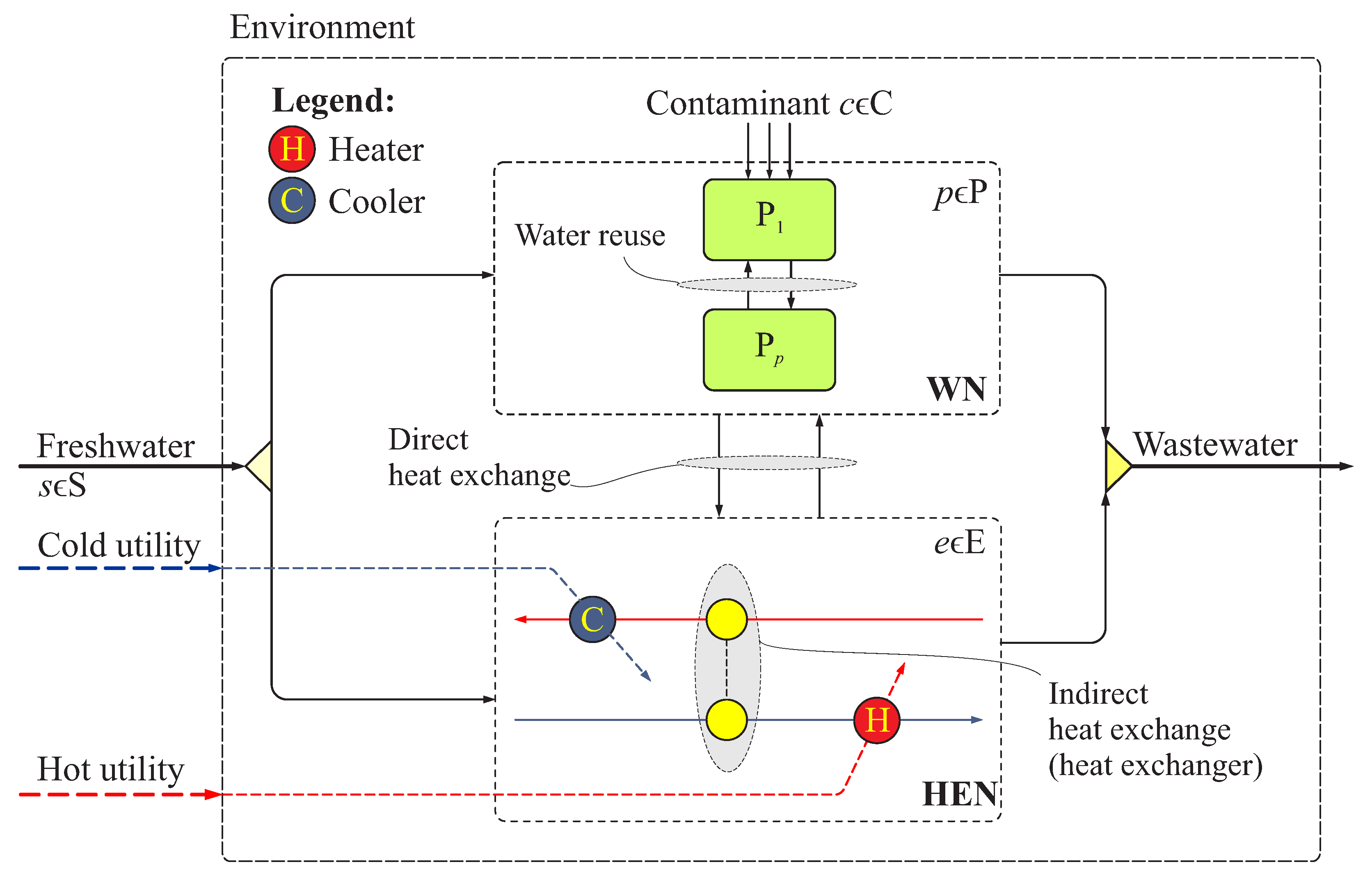
Water and energy are used for various purposes within industrial processes. The minimisation of the consumption of these resources can be achieved by systematically exploring their interconnections in combined water and energy networks or heat-integrated water networks (HIWNs). Various systematic methods (conceptual, mathematical programming and their combination) have been used to achieve this goal. The conceptual methods are based on pinch analysis (PA), and the mathematical programming (MP) methods are based on superstructure optimisation. These methods have been applied to minimise water and energy consumption in various processes. The MP methods, compared to the PA methods, can better address HIWNs, including large-scale problems, multiple contaminants, multiple freshwater sources and gains and losses of water and heat. MP methods have been successfully applied to find the best trade-offs between investment and operating costs in HIWNs.

A work by Budak Duhbacı et al. [1] presented a review of papers considering water and energy minimisation and the improvements achieved in different industrial processes by the application of MP methods. Ahmetović et al. [2] presented a review of systematic methods (PA and MP) along with the the results of case studies in the Kraft pulp mills and reported typical savings in freshwater and energy consumption. The reader is also referred to review papers by Zhang et al. [3], Kermani et al. [4] and Ahmetović et al. [5] for more information about the various methods used for solving HIWN problems.

The focus of several papers have been related to proposing superstructures, models and efficient solution strategies that can be used for solving various HIWN problems, including large-scale ones. Leewongtanawit and Kim [6] proposed a simultaneous design methodology using an MINLP model and solved a large-scale HIWN problem with multiple contaminants and multiple freshwater sources of different temperatures and quality levels. Yang and Grossmann [7] proposed a simultaneous water- and heat-targeting model, combining a water network with a heat-t-argeting model [8] for flowsheet optimisation. This targeting model can be applied to HIWN problems including large-scale problems. Liu et al. [9] proposed a generalised disjunctive programming model (GDP) for the simultaneous inegration of water and energy in HIWNs. This model enables the trade-offs between freshwater and utility consumption and non-isothermal mixing, reducing the complexity of the subsequent heat exchanger network (HEN) design. Ibrić et al. [10] proposed a compact superstructure and an MINLP model for the simultaneous synthesis of HIWNs. The proposed heuristic rules are used for superstructure simplification. The proposed model is solved using a two-step solution strategy that includes targeting and design steps. Hong et al. [11] proposed a systematic simultaneous optimisation approach including a three-step solution strategy that can be used for solving large-scale industrial HIWN problems. In this strategy, a combination of NLP and MINLP models is used to design the HIWN. Ibrić et al. [12] proposed a modified compact superstructure of their previous work [10], an MINLP model and a three-step solution strategy for solving large-scale problems of HIWNs. The modified superstructure includes a simplified heat integration block, enabling non-isothermal mixing and indirect heat exchange within an overall water network with reduced complexity. Recently, Dong et al. [13] proposed a superstructure considering splitters and mixers for every water-using operation and heat exchange unit to simultaneously design HIWNs. The results are presented for a different number of heat exchange units starting from the minimum number of heat exchange units and increasing this number with each iteration.

Based on the published papers, it can be concluded that the majority of them have considered small- and medium-scale HIWN problems, and only several works addressed large-scale HIWN problems. In addition, based on the results reported in the literature for HIWN problems (small-, medium- and large-scale), it can be concluded that the proposed optimal designs have a relatively small number of heat exchangers, compared to traditional HEN designs in which hot and cold process water streams are involved in heat integration. In most cases, there are less than ten heat exchangers in the optimal HIWN designs reported in the literature. One of the reasons for this is that hot and cold water streams in HIWNs can be involved in indirect heat transfers through heat exchangers as well as direct heat transfers by mixing various water streams. Accordingly, due to the mixing of various hot and cold water streams (direct heat transfer), the number of heat exchangers in a final HIWN design can be significantly smaller than a classical HEN design, in which hot and cold process streams are mainly involved in an indirect heat integration.

This work presents a new superstructure and a simultaneous optimisation MINLP model of a heat-integrated water network. In this model, a water network (WN) is combined with a modified HEN model instead of considering a stage-wise HEN superstructure model [14,15] to reduce the overall network complexity and the number of continuous and discrete variables. The stage-wise HEN superstructure [14,15] consists of heat integration stages in which the corresponding stream is split and directed to an exchanger for each potential match between each hot or cold stream. The outlet streams from the exchangers are mixed and the stream is directed to the next stage. The number of stages is usually equal to the maximum number of hot or cold streams. However, the number of possible heat exchange matches increases significantly with the increased number of hot and cold streams. Thus, the overall complexity of the combined HIWN model depends on the identification of hot and cold streams within the WN. In previous research [10], hot and cold streams within the WN were defined with the heating and cooling stages, with a limited number of hot and cold streams directed to the HEN superstructure [14]. The model is later modified to reduce the number of heating/cooling stages [12] using the same HEN superstructure. However, even with the reduced number of hot and cold streams (e.g., a maximum of five), there is still a large number of possible heat-exchange opportunities. Large-scale problems are still difficult to solve and special solution strategies are required, including separate targeting and design steps [12]. The new superstructure proposed in this paper includes a new HEN design consisting of a limited number of heat exchangers and a corresponding number of heaters and coolers, with their interconnections. Additional opportunities for the splitting and mixing of hot and cold water streams are enabled as well as various patterns of heat exchangers (serial, parallel and their combinations) and bypasses. The MINLP model is solved by a one-step solution strategy to minimise the total annualised cost (TAC) of the overall HIWN. This strategy also enables the random generation of initial points, an iterative solution of the MINLP model and the generation of multiple solutions, from which the best one can be chosen. The results obtained for various HIWN problems, including large-scale problems, are in good agreement with the reported literature results.

2. Materials and Methods

2.1. Problem Formulation

Process industries usually require process water that is used in different process operations (process water-using units). Process operations require water of different temperatures and quality, and the water within process operations becomes contaminated in direct contact with the process streams. The wastewater leaving process is discharged into the environment, satisfying a specified temperature constraint. Figure 1 shows a generic representation of the HIWN problem.

The synthesis problem of HIWNs to be solved is stated as follows. The process consists of process water-using units $(p\in P)$ requiring water of different quality and temperature. Within unit p, water becomes contaminated in direct contact with a process stream and, thus, the contaminant $(c\in C)$ is transferred to the water stream. The water is supplied from external freshwater sources ($s\in S$). Freshwater sources can have different temperatures and contaminant concentrations. Water can be reused from the internal water sources (from process unit $P_1$ to process unit $P_p$ and otherwise) within the water network (WN). To supply water at the required temperatures for the process units p, water heating and cooling is required within the HEN. The HEN consists of heat exchangers $(e\in E)$ enabling the maximum heat recovery between hot and cold water streams; thus, the minimum utility consumption at the specified exchanger minimum approach temperature (EMAT) is enabled also. The hot and cold utilities are available for additional heating and cooling to satisfy the target temperatures of hot and cold streams. The wastewater is discharged into the environment at the specified temperature. It is required to determine the optimum design of the HIWN to minimise the TAC. The network design should include the optimal connections between freshwater sources, process water-using units and heat exchangers and the optimal number of heat exchangers.

2.2. Motivation Example

As a motivation example, a simple problem is presented consisting of two process water-using units and a single contaminant. Freshwater is at temperature of 20 °C and wastewater is discharged into the environment at 30 °C. The data for this example are presented in

Table 1. Process water-using units data for motivation example.

Unit	${\mathit{L}}_{\mathit{p},\mathit{c}}$ (g/s)	${\mathit{x}}_{\mathit{p},\mathit{c}}^{(\mathit{in},\mathit{max})}$ (ppm)	${\mathit{x}}_{\mathit{p},\mathit{c}}^{(\mathit{out},\mathit{max})}$ (ppm)	${\mathit{t}}_{\mathit{p}}$ (°C)
$P_1$	5	50	100	100
$P_2$	30	50	800	75

, including the mass load of contaminant c in the process unit p ($L_{p,c}$), the maximum inlet $x_{p,c}^{(in,max)}$ and outlet $x_{p,c}^{(out,max)}$ concentrations of contaminant c and the operating temperature $t_p$ of the process water-using unit p. The cost data required for this problem and all other problems solved in this paper are the same.

If water integration is not considered, freshwater is used in $P_1$ and $P_2$ in a total amount of 87.5 kg/s. The water required by water-using units is at 100 °C and 75 °C, and the heating of freshwater is necessary by using external hot utility, if no heat integration is considered. Moreover, to satisfy the temperature constraint of the wastewater, the streams leaving the process water-using units need to be cooled. Thus, the consumption of hot and cold utilities is 25,462.5 kW and 21,787.5 kW, respectively. The basic design, without the water and heat integration, is given in Figure 2.

To reduce freshwater use, water reuse opportunities between process water-using units need to be considered. The water leaving $P_1$ with contaminant concentration 100 ppm can be partially reused in $P_2$ when mixed with freshwater to reduce contaminant concentration to the 50 ppm required at the $P_2$ inlet. It is clear from Figure 2 that the energy of the hot streams leaving the process units can be used to a certain degree, depending on the temperature approach, to preheat cold freshwater streams. Thus, the heat integration opportunities can also be considered to maximise heat recovery. Performing an optimisation of the HIWN using mathematical programming by minimising the TAC, an optimal design shown in Figure 3 can be obtained with reduced freshwater consumption (70 kg/s vs. 87.5 kg/s). The freshwater consumption is reduced due to water reuse $P_1\to P_2$ in the amount of 20 kg/s. The utilities’ consumption is significantly lower for the hot (2940 kW vs. 25,462.5 kW) and the cold utility (0 kW vs. 21,787.5 kW), due to heat integration. The energy of the effluent stream (14,112 kW) is utilised to preheat freshwater from 20 °C to 68 °C. Additionally, the energy of the stream leaving $P_1$ (3780 kW) is used to additionally preheat freshwater from 68 °C to 86 °C. The hot utility (2940 kW) is required to achieve the operating temperature of $P_1$ (100 °C). An investment cost of heat exchangers for the integrated design is somewhat higher (USD 248,188/year vs. USD 229,751/year) than the base case due to higher heat exchange areas resulting from a lower temperature difference at the hot and the cold sides of the heat exchangers. The TAC of the integrated design is USD 2,112,569/year, obtained by the later-proposed model and solution approach. The solution obtained in the literature [16] by using the MINLP model (538 equations, 427 continuous variables, 92 discrete variables) proposed by Ahmetović and Kravanja [17] and the global optimisation solver BARON exhibits the same network design. The proposed model for this example consists of 118 single equations, 228 continuous variables and 9 discrete variables.

2.3. Superstructure

Figure 4 shows a generic design of the proposed HIWN superstructure. The superstructure consists of:

• freshwater sources $s\in S=\left\{S_1,S_2,\dots S_s\right\}$;
• proces water-using units $p\in P=\left\{P_1,P_2,\dots P_p\right\}$;
• heat exchanger units $e\in E=\left\{E_1,E_2,\dots E_e\right\}$, with the corresponding heaters and coolers;
• wastewater, discharged into the environment.

The elements of the superstructure within each of the blocks consist of mixers and/or splitters that enable their connections within and between the blocks. These connections enable multiple options for water reuse. Options for heat exchange include direct heat exchange through the non-isothermal mixing, as well as indirect heat exchange within heat exchangers, heaters and coolers. To each heat exchanger $e\in E$, one heater and one cooler are assigned for additional heating and cooling of the water streams.

2.4. Model

This section describes the proposed model for the HIWN superstructure shown in Figure 4. The model consists of the mass and heat balance of the WN and HEN superstructure elements as well as additional heat transfer constraints within the HEN. The model is developed under the following assumptions:

• Temperature and contaminant concentrations of the freshwater source s are constant;
• The temperature at the inlet/outlet of the process unit p is constant;
• The specific heat capacity of the water streams is constant;
• The flowrate of water through the process unit p is constant, under the assumption that the mass of the contaminants in the water streams is much lower than the overall mass of the water streams;
• The process unit p operates at constant mass load of contaminants transferred to the water stream;
• The individual heat transfer coefficients of hot and cold water streams and utilities are constant;
• Heat losses to the environment are neglected;
• Single hot and cold utilities are available at constant inlet/outlet temperatures;
• Counter-current heat exchange is assumed;
• Water is at liquid state, and no phase change occurs for the water streams;
• The process operates continuously in steady state conditions.

2.4.1. Freshwater Splitter

The freshwater splitter with the corresponding streams is shown in Figure 5. The mass balance of the freshwater splitter $s\in S$ is given by Equation (1).

$$m_s=\sum _p{m}_{s,p}+\sum _e{m}_{s,e}^{\left(hs\right)}+\sum _e{m}_{s,e}^{\left(cs\right)}+\sum _e{m}_{s,e}^{\left(H\right)}+\sum _e{m}_{s,e}^{\left(C\right)},\forall s\in S$$

(1)

2.4.2. Water-Using Unit

The process water-using unit $p\in P$, with the corresponding water streams, is shown in Figure 6. The overall mass balance and the mass balance of contaminant $c\in C$ for the process unit $p\in P$ mixer is given by Equations (2) and (3).

$$m_p^{\left(in\right)}=\sum _s{m}_{s,p}+\sum _e{m}_{e,p}^{\left(hs\right)}+\sum _e{m}_{e,p}^{\left(cs\right)}+\sum _{\begin{array}{c}{p}^{\prime }\\ p\ne p^{\prime }\end{array}}{m}_{p^{\prime },p}+\sum _e{m}_{e,p}^{\left(C\right)}+\sum _e{m}_{e,p}^{\left(H\right)},\forall p\in P$$

(2)

$$\begin{array}{cc}\hfill m_p^{\left(in\right)}{x}_{p,c}^{\left(in\right)}& \hfill =\sum _s{m}_{s,p}{x}_{s,c}+\sum _e{m}_{e,p}^{\left(hs\right)}{x}_{e,c}^{\left(hs\right)}+\sum _e{m}_{e,p}^{\left(cs\right)}{x}_{e,c}^{\left(cs\right)}+\sum _{\begin{array}{c}{p}^{\prime }\\ p\ne p^{\prime }\end{array}}{m}_{p^{\prime },p}{x}_{p^{\prime },c}^{\left(out\right)}\hfill \\ \hfill & \hfill +\sum _e{m}_{e,p}^{\left(C\right)}{x}_{e,c}^{\left(C\right)}+\sum _e{m}_{e,p}^{\left(H\right)}{x}_{e,c}^{\left(H\right)},\forall p\in P,\forall c\in C\hfill \end{array}$$

(3)

The heat balance of the process unit p mixer is given by Equation (4).

$$\begin{array}{cc}\hfill m_p^{\left(in\right)}{t}_p^{\left(in\right)}& \hfill =\sum _s{m}_{s,p}{t}_s+\sum _e{m}_{e,p}^{\left(hs\right)}{t}_e^{(hs,out)}+\sum _e{m}_{e,p}^{\left(cs\right)}{t}_e^{(cs,out)}+\sum _{\begin{array}{c}{p}^{\prime }\\ p\ne p^{\prime }\end{array}}{m}_{p^{\prime },p}{t}_{p^{\prime }}^{\left(out\right)}\hfill \\ \hfill & \hfill +\sum _e{m}_{e,p}^{\left(C\right)}{t}_e^{(C,out)}+\sum _e{m}_{e,p}^{\left(H\right)}{t}_e^{(H,out)},\forall p\in P\hfill \end{array}$$

(4)

Under the assumption that the mass of contaminants in the water streams is much lower than the overall mass, the flow-rate of water at the inlet and outlet of the process water-using unit p is equal, as given by Equation (5). However, the concentration of contaminant c is increased as the mass load of contaminant $L_{p,c}$ is transferred to the water stream within the process unit p, as given by Equation (6).

$$m_p^{\left(in\right)}=m_p^{\left(out\right)},\forall p\in P$$

(5)

$$m_p^{\left(in\right)}{x}_{p,c}^{\left(in\right)}+L_{p,c}=m_p^{\left(out\right)}{x}_{p,c}^{\left(out\right)},\forall p\in P,\forall c\in C$$

(6)

The mass balance of the process unit p splitter is given by Equation (7).

$$m_p^{\left(out\right)}=\sum _{\begin{array}{c}{p}^{\prime }\\ p\ne p^{\prime }\end{array}}{m}_{p,p^{\prime }}+\sum _e{m}_{p,e}^{\left(hs\right)}+\sum _e{m}_{p,e}^{\left(cs\right)}+\sum _e{m}_{p,e}^{\left(C\right)}+\sum _e{m}_{p,e}^{\left(H\right)}+m_p^{\left(env\right)},\forall p\in P$$

(7)

2.4.3. Heat Exchangers

Figure 7 shows a counter-current heat exchanger with the corresponding hot and cold streams. The exchanger $e\in E$ consists of an exchanger hot stream mixer and splitter as well as a cold stream mixer and splitter. The selection of mixers in front of heat exchangers enables the possibility that any water stream within the network can be directed towards any heat exchanger as a hot and/or cold stream. The number of heat exchangers is set arbitrarily and the existence of multiple heat exchangers enables many options for heat exchange (serial, parallel, bypass and their combination), as there are interconnections between individual heat exchangers. The overall mass balance and the mass balance for each contaminant $c\in C$ for the exchanger $e\in E$ hot stream mixer is given by Equations (8) and (9).

$$m_e^{\left(hs\right)}=\sum _p{m}_{p,e}^{\left(hs\right)}+\sum _s{m}_{s,e}^{\left(hs\right)}+\sum _{\begin{array}{c}{e}^{\prime }\\ e\ne e^{\prime }\end{array}}{m}_{e^{\prime },e}^{\left(hs\right)}+\sum _{\begin{array}{c}{e}^{\prime }\\ e\ne e^{\prime }\end{array}}{m}_{e^{\prime },e}^{(cs,hs)},\forall e\in E$$

(8)

$$m_e^{\left(hs\right)}{x}_{e,c}^{\left(hs\right)}=\sum _p{m}_{p,e}^{\left(hs\right)}{x}_{p,c}^{\left(out\right)}+\sum _s{m}_{s,e}^{\left(hs\right)}{x}_{s,c}+\sum _{\begin{array}{c}{e}^{\prime }\\ e\ne e^{\prime }\end{array}}{m}_{e^{\prime },e}^{\left(hs\right)}{x}_{e^{\prime },c}^{\left(hs\right)}+\sum _{\begin{array}{c}{e}^{\prime }\\ e\ne e^{\prime }\end{array}}{m}_{e^{\prime },e}^{(cs,hs)}{x}_{e^{\prime },c}^{\left(cs\right)},\forall e\in E,\forall c\in C$$

(9)

The heat balance of the exchanger $e\in E$ hot stream mixer is given by Equation (10).

$$m_e^{\left(hs\right)}{t}_e^{(hs,in)}=\sum _p{m}_{p,e}^{\left(hs\right)}{t}_p^{\left(out\right)}+\sum _s{m}_{s,e}^{\left(hs\right)}{t}_s+\sum _{\begin{array}{c}{e}^{\prime }\\ e\ne e^{\prime }\end{array}}{m}_{e^{\prime },e}^{\left(hs\right)}{t}_{e^{\prime }}^{(hs,out)}+\sum _{\begin{array}{c}{e}^{\prime }\\ e\ne e^{\prime }\end{array}}{m}_{e^{\prime },e}^{(cs,hs)}{t}_{e^{\prime }}^{(cs,out)},\forall e\in E$$

(10)

The mass balance of exchanger $e\in E$ hot stream splitter is given by Equation (11).

$$m_e^{\left(hs\right)}=m_e^{(hs,env)}+\sum _p{m}_{e,p}^{\left(hs\right)}+\sum _{\begin{array}{c}{e}^{\prime }\\ e\ne e^{\prime }\end{array}}{m}_{e,e^{\prime }}^{\left(hs\right)}+\sum _{\begin{array}{c}{e}^{\prime }\\ e\ne e^{\prime }\end{array}}{m}_{e,e^{\prime }}^{(hs,cs)}+\sum _{e^{\prime }}{m}_{e,e^{\prime }}^{(hs,C)},\forall e\in E$$

(11)

The overall mass balance and the mass balance for each contaminant $c\in C$ for the exchanger $e\in E$ cold stream mixer is given by Equations (12) and (13). The heat balance of the exchanger $e\in E$ cold stream mixer is given by Equation (14).

$$m_e^{\left(cs\right)}=\sum _p{m}_{p,e}^{\left(cs\right)}+\sum _s{m}_{s,e}^{\left(cs\right)}+\sum _{\begin{array}{c}{e}^{\prime }\\ e\ne e^{\prime }\end{array}}{m}_{e^{\prime },e}^{\left(cs\right)}+\sum _{\begin{array}{c}{e}^{\prime }\\ e\ne e^{\prime }\end{array}}{m}_{e^{\prime },e}^{(hs,cs)},\forall e\in E$$

(12)

$$m_e^{\left(cs\right)}{x}_{e,c}^{\left(cs\right)}=\sum _p{m}_{p,e}^{\left(cs\right)}{x}_{p,c}^{\left(out\right)}+\sum _s{m}_{s,e}^{\left(cs\right)}{x}_{s,c}+\sum _{\begin{array}{c}{e}^{\prime }\\ e\ne e^{\prime }\end{array}}{m}_{e^{\prime },e}^{\left(cs\right)}{x}_{e^{\prime },c}^{\left(cs\right)}+\sum _{\begin{array}{c}{e}^{\prime }\\ e\ne e^{\prime }\end{array}}{m}_{e^{\prime },e}^{(hs,cs)}{x}_{e^{\prime },c}^{\left(hs\right)},\forall e\in E,\forall c\in C$$

(13)

$$m_e^{\left(cs\right)}{t}_e^{(cs,in)}=\sum _p{m}_{p,e}^{\left(cs\right)}{t}_p^{\left(out\right)}+\sum _s{m}_{s,e}^{\left(cs\right)}{t}_s+\sum _{\begin{array}{c}{e}^{\prime }\\ e\ne e^{\prime }\end{array}}{m}_{e^{\prime },e}^{\left(cs\right)}{t}_{e^{\prime }}^{(cs,out)}+\sum _{\begin{array}{c}{e}^{\prime }\\ e\ne e^{\prime }\end{array}}{m}_{e^{\prime },e}^{(hs,cs)}{t}_{e^{\prime }}^{(hs,out)},\forall e\in E$$

(14)

The mass balance of exchanger $e\in E$ cold stream splitter is given by Equation (15).

$$m_e^{\left(cs\right)}=m_e^{(cs,env)}+\sum _p{m}_{e,p}^{\left(cs\right)}+\sum _{\begin{array}{c}{e}^{\prime }\\ e\ne e^{\prime }\end{array}}{m}_{e,e^{\prime }}^{\left(cs\right)}+\sum _{\begin{array}{c}{e}^{\prime }\\ e\ne e^{\prime }\end{array}}{m}_{e,e^{\prime }}^{(cs,hs)}+\sum _{e^{\prime }}{m}_{e,e^{\prime }}^{(cs,H)},\forall e\in E$$

(15)

2.4.4. Coolers and Heaters

According to the proposed superstructure shown in Figure 4, to each heat exchanger $e\in E$, one heater (H) is assigned for additional heating of the cold streams and one cooler (C) for additional cooling of the hot streams. Figure 8 shows the cooler and heater with their corresponding streams. The overall mass balance and the mass balance for each contaminant $c\in C$ for the cooler $e\in E$ mixer is given by Equations (16) and (17). The heat balance of the cooler $e\in E$ mixer is given by Equation (18).

$$m_e^{\left(C\right)}=\sum _p{m}_{p,e}^{\left(C\right)}+\sum _s{m}_{s,e}^{\left(C\right)}+\sum _{\begin{array}{c}{e}^{\prime }\\ e\ne e^{\prime }\end{array}}{m}_{e^{\prime },e}^{\left(C\right)}+\sum _{e^{\prime }}{m}_{e^{\prime },e}^{(hs,C)},\forall e\in E$$

(16)

$$m_e^{\left(C\right)}{x}_{e,c}^{\left(C\right)}=\sum _p{m}_{p,e}^{\left(C\right)}{x}_{p,c}^{\left(out\right)}+\sum _s{m}_{s,e}^{\left(C\right)}{x}_{s,c}+\sum _{\begin{array}{c}{e}^{\prime }\\ e\ne e^{\prime }\end{array}}{m}_{e^{\prime },e}^{\left(C\right)}{x}_{e^{\prime },c}^{\left(C\right)}+\sum _{e^{\prime }}{m}_{e^{\prime },e}^{(hs,C)}{x}_{e,c}^{\left(hs\right)},\forall e\in E,\forall c\in C$$

(17)

$$m_e^{\left(C\right)}{t}_e^{(C,in)}=\sum _p{m}_{p,e}^{\left(C\right)}{t}_p^{\left(out\right)}+\sum _s{m}_{s,e}^{\left(C\right)}{t}_s+\sum _{\begin{array}{c}{e}^{\prime }\\ e\ne e^{\prime }\end{array}}{m}_{e^{\prime },e}^{\left(C\right)}{t}_{e^{\prime }}^{(C,out)}+\sum _{e^{\prime }}{m}_{e^{\prime },e}^{(hs,C)}{t}_{e^{\prime }}^{(hs,out)},\forall e\in E$$

(18)

The mass balance of the cooler $e\in E$ splitter is given by Equation (19).

$$m_e^{\left(C\right)}=\sum _p{m}_{e,p}^{\left(C\right)}+m_e^{(C,env)}+\sum _{\begin{array}{c}{e}^{\prime }\\ e\ne e^{\prime }\end{array}}{m}_{e,e^{\prime }}^{\left(C\right)},\forall e\in E$$

(19)

The overall mass balance and the mass balance for each $c\in C$ for the heater $e\in E$ mixer is given by Equations (20) and (21). The heat balance of the heater $e\in E$ mixer is given by Equation (22).

$$m_e^{\left(H\right)}=\sum _p{m}_{p,e}^{\left(H\right)}+\sum _s{m}_{s,e}^{\left(H\right)}+\sum _{\begin{array}{c}{e}^{\prime }\\ e\ne e^{\prime }\end{array}}{m}_{e^{\prime },e}^{\left(H\right)}+\sum _{e^{\prime }}{m}_{e^{\prime },e}^{(cs,H)},\forall e\in E$$

(20)

$$m_e^{\left(H\right)}{x}_{e,c}^{\left(H\right)}=\sum _p{m}_{p,e}^{\left(H\right)}{x}_{p,c}^{\left(out\right)}+\sum _s{m}_{s,e}^{\left(H\right)}{x}_{s,c}+\sum _{\begin{array}{c}{e}^{\prime }\\ e\ne e^{\prime }\end{array}}{m}_{e^{\prime },e}^{\left(H\right)}{x}_{e^{\prime },c}^{\left(H\right)}+\sum _{e^{\prime }}{m}_{e^{\prime },e}^{(cs,H)}{x}_{e,c}^{\left(cs\right)},\forall e\in E,\forall c\in C$$

(21)

$$m_e^{\left(H\right)}{t}_e^{(H,in)}=\sum _p{m}_{p,e}^{\left(H\right)}{t}_p^{\left(out\right)}+\sum _s{m}_{s,e}^{\left(H\right)}{t}_s+\sum _{\begin{array}{c}{e}^{\prime }\\ e\ne e^{\prime }\end{array}}{m}_{e^{\prime },e}^{\left(H\right)}{t}_{e^{\prime }}^{(H,out)}+\sum _{e^{\prime }}{m}_{e^{\prime },e}^{(cs,H)}{t}_{e^{\prime }}^{(cs,out)},\forall e\in E$$

(22)

The mass balance of the heater $e\in E$ splitter is given by Equation (23).

$$m_e^{\left(H\right)}=\sum _p{m}_{e,p}^{\left(H\right)}+m_e^{(H,env)}+\sum _{\begin{array}{c}{e}^{\prime }\\ e\ne e^{\prime }\end{array}}{m}_{e,e^{\prime }}^{\left(H\right)},\forall e\in E$$

(23)

2.4.5. Wastewater Mixer

The streams entering the wastewater mixer are those leaving all the splitters in the water network except the freshwater splitter, as shown in Figure 9. The overall mass balance of the wastewater mixer and the mass balance for the contaminant $c\in C$ are given by Equations (24) and (25). The heat balance of the wastewater mixer is given by Equation (26).

$$m^{\left(env\right)}=\sum _p{m}_p^{\left(env\right)}+\sum _e{m}_e^{(cs,env)}+\sum _e{m}_e^{(hs,env)}+\sum _e{m}_e^{(C,env)}+\sum _e{m}_e^{(H,env)},\forall e\in E$$

(24)

$$\begin{array}{cc}\hfill m^{\left(env\right)}{x}_c^{\left(env\right)}& \hfill =\sum _p{m}_p^{\left(env\right)}{x}_{p,c}^{\left(out\right)}+\sum _e{m}_e^{(cs,env)}{x}_{e,c}^{\left(cs\right)}+\sum _e{m}_e^{(hs,env)}{x}_{e,c}^{\left(hs\right)}\hfill \\ \hfill & \hfill +\sum _e{m}_e^{(C,env)}{x}_{e,c}^{\left(C\right)}+\sum _e{m}_e^{(H,env)}{x}_{e,c}^{\left(H\right)},\forall e\in E,\forall c\in C\hfill \end{array}$$

(25)

$$\begin{array}{cc}\hfill m^{\left(env\right)}{t}^{\left(env\right)}& \hfill {\displaystyle =\sum _p{m}_p^{\left(env\right)}{t}_p^{\left(out\right)}+\sum _e{m}_e^{(cs,env)}{t}_e^{(cs,out)}+\sum _e{m}_e^{(hs,env)}{t}_e^{(hs,out)}}\hfill \\ \hfill & \hfill {\displaystyle +\sum _e{m}_e^{(C,env)}{t}_e^{(C,out)}+\sum _e{m}_e^{(H,env)}{t}_e^{(H,out)},\forall e\in E}\hfill \end{array}$$

(26)

2.4.6. Global Mass Balance

According to Karuppiah and Grossmann [18], the global mass balance equations can improve the lower bounds of the relaxed model. The overall mass balance and the contaminant mass balance are given by Equations (27) and (28).

$$\sum _s{m}_s=m^{\left(env\right)}$$

(27)

$$\sum _s{m}_s{x}_{s,c}+\sum _p{L}_{p,c}=m^{\left(env\right)}{x}_c^{\left(env\right)},\forall c\in C$$

(28)

2.4.7. Heat Transfer Constraints

Within the heat exchanger $e\in E$, heat transfer occurs between the hot and cold water streams. The heat allocated from the hot water stream $\left(q_e\right)$ is given by Equation (29). The same amount of heat $\left(q_e\right)$ is allocated to the cold water stream as the heat losses are neglected, as given by Equation (30).

$$q_e=m_e^{\left(hs\right)}{c}_p\left(t_e^{(hs,in)}-t_e^{(hs,out)}\right),\forall e\in E$$

(29)

$$q_e=m_e^{\left(cs\right)}{c}_p\left(t_e^{(cs,out)}-t_e^{(cs,in)}\right),\forall e\in E$$

(30)

The heat balance of the cooler and heater are given by Equations (31) and (32).

$$q_e^{\left(C\right)}=m_e^{\left(C\right)}{c}_p\left(t_e^{(C,in)}-t_e^{(C,out)}\right),\forall e\in E$$

(31)

$$q_e^{\left(H\right)}=m_e^{\left(H\right)}{c}_p\left(t_e^{(H,out)}-t_e^{(H,in)}\right),\forall e\in E$$

(32)

By assuming counter-current heat exchangers with the upper bound on temperature differences $\Gamma$, the temperature differences at the hot and cold sides of the heat exchangers, the coolers and the heaters are given by Equations (33)–(38).

$$\Delta t{h}_e\le t_e^{(hs,in)}-t_e^{(cs,out)}+\Gamma \left(1-z_e\right),\forall e\in E$$

(33)

$$\Delta t{c}_e\le t_e^{(hs,out)}-t_e^{(cs,in)}+\Gamma \left(1-z_e\right),\forall e\in E$$

(34)

$$\Delta t{h}_e^{\left(C\right)}\le t_e^{(C,in)}-t^{(CU,out)}+\Gamma \left(1-z_e^{\left(C\right)}\right),\forall e\in E$$

(35)

$$\Delta t{c}_e^{\left(C\right)}\le t_e^{(C,out)}-t^{(CU,in)}+\Gamma \left(1-z_e^{\left(C\right)}\right),\forall e\in E$$

(36)

$$\Delta t{h}_e^{\left(H\right)}\le t^{(HU,in)}-t_e^{(H,out)}+\Gamma \left(1-z_e^{\left(H\right)}\right),\forall e\in E$$

(37)

$$\Delta t{c}_e^{\left(H\right)}\le t^{(HU,out)}-t_e^{(H,in)}+\Gamma \left(1-z_e^{\left(H\right)}\right),\forall e\in E$$

(38)

Equations (39)–(42) describe the feasibility of temperatures of water streams entering and leaving the heat exchangers, heaters and coolers.

$$t_e^{(hs,in)}\ge t_e^{(hs,out)},\forall e\in E$$

(39)

$$t_e^{(cs,in)}\le t_e^{(cs,out)},\forall e\in E$$

(40)

$$t_e^{(H,in)}\le t_e^{(H,out)},\forall e\in E$$

(41)

$$t_e^{(C,in)}\ge t_e^{(C,out)},\forall e\in E$$

(42)

With the binary variables $z_e,z_e^{\left(C\right)},z_e^{\left(H\right)}$ denoting the existence of heat exchangers, coolers and heaters, the heat transfer is constrained by the upper bounds by the following Equations (43)–(45).

$$q_e-q_e^{\left(up\right)}{z}_e\le 0,\forall e\in E$$

(43)

$$q_e^{\left(C\right)}-q_e^{(C,up)}{z}_e^{\left(C\right)}\le 0,\forall e\in E$$

(44)

$$q_e^{\left(H\right)}-q_e^{(H,up)}{z}_e^{\left(H\right)}\le 0,\forall e\in E$$

(45)

2.4.8. Objective Function of the Model

The objective function of the model minimises the TAC of the network consisting of freshwater cost, hot and cold utility cost and the investment cost of HEN, as given by Equation (46)

$$\begin{array}{cc}\hfill minTAC& =\sum _s{m}_{s}CF{W}_{s}f+\sum _e{q}_e^{\left(H\right)}{C}_{HU}+\sum _e{q}_e^{\left(C\right)}{C}_{CU}+\sum _e\left(a{z}_e+b{A}_e^n\right)\hfill \\ & +\sum _e\left(a{z}_e^{\left(C\right)}+b{\left(A_e^{\left(C\right)}\right)}^n\right)+\sum _e\left(a{z}_e^{\left(H\right)}+b{\left(A_e^{\left(H\right)}\right)}^n\right)\hfill \end{array}$$

(46)

where the heat exchanger and the cooler and heater heat exchange area parameters are given as follows:

$$A_e=\frac{q_e\left({\displaystyle \frac{1}{h_e^{\left(hs\right)}}+\frac{1}{h_e^{\left(cs\right)}}}\right)}{{\left({\displaystyle \Delta t{h}_e\Delta t{c}_e\frac{\Delta t{h}_e+\Delta t{c}_e}{2}}\right)}^{1/3}}$$

(47)

$$A_e^{\left(C\right)}=\frac{q_e^{\left(C\right)}\left({\displaystyle \frac{1}{h_e^{\left(hs\right)}}+\frac{1}{h_{CU}}}\right)}{{\left({\displaystyle \Delta t{h}_e^{\left(C\right)}\Delta t{c}_e^{\left(C\right)}\frac{\Delta t{h}_e^{\left(C\right)}+\Delta t{c}_e^{\left(C\right)}}{2}}\right)}^{1/3}}$$

(48)

$$A_e^{\left(H\right)}=\frac{q_e^{\left(H\right)}\left({\displaystyle \frac{1}{h_e^{\left(cs\right)}}+\frac{1}{h_{HU}}}\right)}{{\left({\displaystyle \Delta t{h}_e^{\left(H\right)}\Delta t{c}_e^{\left(H\right)}\frac{\Delta t{h}_e^{\left(H\right)}+\Delta t{c}_e^{\left(H\right)}}{2}}\right)}^{1/3}}$$

(49)

Chen’s [19] approximation of the logarithmic mean temperature difference was used in Equations (47)–(49) to avoid numerical problems with the logarithmic term. Chen’s approximation slightly overestimates the heat exchange area requirements [20], on average by 0.025% in the studied examples.

2.5. Solution Strategy

The model is implemented in the General Algebraic Modelling System (GAMS) v. 24.6.1 [21] and solved on a laptop computer with a 2.80 GHz processor (4 cores) and 16 GB RAM. The proposed model is solved by using a one-step iterative strategy. For the solution of the MINLP model, the SBB solver is used with CONOPT as NLP solvers for the root node and sub-nodes. Multiple solutions are generated by solving the same model iteratively by generating different initialisation points for all variables on each solve run. Initialisation points are randomly generated for variables between zero and the upper bound for each variable using the GAMS function uniform and generating different initial values in each solve run (execseed = gmillisec(jnow)). Generic upper bounds are obtained based on the initial data from the problem formulation, as proposed by Ibrić et al. [10].

3. Results and Discussion

To demonstrate the capabilities of the proposed model, five examples are solved in increasing order of complexity, concerning a number of process water-using units, contaminants and freshwater sources. The following data are used for the solutions of the problems.

Freshwater: The freshwater is at a temperature of either 20 °C or 30 °C, with a unit cost of USD 0.375/t. The specific heat capacity of all water streams is 4.2 kJ/(kgK). The freshwater is free of contaminants.

Utility: The hot utility is fresh steam at either 120 °C or 150 °C, with unit costs of USD 377/(kW-year) and USD 388/(kW-year). The inlet and outlet temperatures of the hot utility are the same. The cold utility is cooling water at an inlet temperature of 10 °C and an outlet temperature of 20 °C. The unit cost of cooling the water is USD 189/(kW-year).

Heat exchangers: The individual heat transfer coefficients for the hot and cold water streams and the hot and cold utilities are 1 kW/(m²K). The heat exchangers are counter-current with annualised investment cost (USD/year) given as a function of the heat exchange area (m²) as follows: $8000+1200{\left(A\right)}^{0.6}$.

The plant operates continuously 8000 h/year.

3.1. Example 1

This example presents a single-contaminant problem with four process water-using units previously studied in the literature [17,22,23,24]. The freshwater is at 20 °C without contaminants and the wastewater is discharged into the environment at 30 °C. The data for the process water-using units are given in

Table 2. Process water-using units data for Example 1.

Unit	${\mathit{L}}_{\mathit{p},\mathit{c}}$ (g/h)	${\mathit{x}}_{\mathit{p},\mathit{c}}^{(\mathit{i}\mathit{n},\mathit{m}\mathit{a}\mathit{x})}$ (ppm)	${\mathit{x}}_{\mathit{p},\mathit{c}}^{(\mathit{o}\mathit{u}\mathit{t},\mathit{m}\mathit{a}\mathit{x})}$ (ppm)	${\mathit{t}}_{\mathit{p}}$ (°C)
$P_1$	2000	0	100	40
$P_2$	5000	50	100	100
$P_3$	30,000	50	800	75
$P_4$	4000	400	800	50

.

The optimal network design, shown in Figure 10, exhibited the minimum freshwater consumption (25 kg/s) and consumption of only the hot utility (1050 kW). The optimal HEN design consists of two heat exchangers and one heater, with the HEN investment cost of USD 131,525/year. This is a somewhat improved solution compared to the solution obtained by using a more complex stage-wise HEN superstructure combined with the water network superstructure [23]. The same network design and TAC were obtained by Yan et al. [24] by using the NLP model and the global optimisation solver BARON. A comparison of the results with those from the literature for Example 1 is given in

Table 3. Comparison of the results with those from the literature for Example 1.

Reference	Freshwater (kg/s)	Hot Utility (kW)	No. of HEs	HEN Investment (USD/year)	TAC (USD/year)
Bogataj and Bagajewicz [22] *	25	1050	3	146,748	812,598
Ahmetović and Kravanja [17]	25	1050	2	134,227	800,077
Yan et al. [24]	25	1050	3	131,525	797,375
Ibrić et al. [23]	25	1050	2	134,227	800,077
This paper	25	1050	3	131,527	797,377

* Recalculated in Ahmetović and Kravanja [17].

.

3.2. Example 2

In this example, a problem originally solved as an isothermal water network problem [18] is modified as a non-isothermal water network problem, as reported in the literature [25]. The problem includes four process water-using units with two contaminants and a single freshwater source at 20 °C without contaminants. The wastewater is discharged into the environment at 30 °C with no restrictions on contaminant concentrations in the effluent stream. Data for the process water-using units are given in

Table 4. Process water-using units data for Example 2.

Unit	${\mathit{L}}_{\mathit{p},\mathit{c}}$ (kg/h)		${\mathit{x}}_{\mathit{p},\mathit{c}}^{(\mathit{i}\mathit{n},\mathit{m}\mathit{a}\mathit{x})}$ (ppm)		${\mathit{x}}_{\mathit{p},\mathit{c}}^{(\mathit{o}\mathit{u}\mathit{t},\mathit{m}\mathit{a}\mathit{x})}$ (ppm)		${\mathit{t}}_{\mathit{p}}$ (°C)
	A	B	A	B	A	B
$P_1$	1	1.5	0	0	25	37.5	40
$P_2$	1	1	50	50	70	70	50
$P_3$	1	1	50	50	66.667	66.667	75
$P_4$	2	1	50	50	78.571	78.571	100

. The EMAT is 1 °C.

Ibrić et al. [25] reported a solution with the freshwater consumption of 19.444 kg/s and the hot-utlity consumption of 816.67 kW. The network exhibited a design comprising of two heat exchangers and one heater, with the HEN investment cost of USD 188,801/year. The TAC of the network was USD 706,687.7/year. The optimal design shown in Figure 11 exhibited slightly increased consumption of freshwater compared to the literature [25] (20.698 vs. 19.444 kg/s). Consequently, the consumption of hot utility is also increased (869.33 vs. 816.67 kW). However, as a trade-off exist, the HEN investment cost is reduced by ≈41% (USD 111,207 vs. USD 188,801/year). The TAC of the network (USD 662,489/year) is reduced by 6.25% compared to the literature [25].

3.3. Example 3

This example is slightly more complex than the previous one, considering a number of contaminants. The problem consists of four process water-using units and three contaminants originally solved in the literature [22] and later studied by other authors [10,24,26]. The data for the process water-using units are given in

Table 5. Process water-using units data for Example 3.

Unit	${\mathit{L}}_{\mathit{p},\mathit{c}}$ (kg/h)			${\mathit{x}}_{\mathit{p},\mathit{c}}^{(\mathit{i}\mathit{n},\mathit{m}\mathit{a}\mathit{x})}$ (ppm)			${\mathit{x}}_{\mathit{p},\mathit{c}}^{(\mathit{o}\mathit{u}\mathit{t},\mathit{m}\mathit{a}\mathit{x})}$ (ppm)			${\mathit{t}}_{\mathit{p}}$ (°C)
	A	B	C	A	B	C	A	B	C
$P_1$	2	1	3	0	15	0	100	100	100	40
$P_2$	5	0	15	50	100	30	100	200	250	100
$P_3$	30	4	0	100	100	100	800	750	600	75
$P_4$	4	22	17	400	380	250	800	800	800	50

. The freshwater is available at 20 °C without contaminants and the wastewater is discharged into the environment at 30 °C. The EMAT is 1 °C.

The optimal network design obtained by using the model proposed in this paper is shown in Figure 12. Compared to the network design in the literature [10], the basic design, the freshwater and hot utility consumption and the heat integration opportunities are the same. The only difference is related to the water reuse opportunities related to $P_4$, due to the increased flowrate in $P_4$.

Table 6. Comparison of the results with those from the literature for Example 3.

Reference	Freshwater (kg/s)	Hot Utility (kW)	No. of HEs	HEN Investment (USD/year)	TAC (USD/year)
Bogataj and Bagajewicz [22] *	26.535	1115.7	4	199,861	907,066
Ahmetović and Kravanja [26]	26.535	1114.5	4	183,063	889,772
Yan et al. [24]	26.716	1122.1	4	183,107	894,856
Ibrić et al. [10]	26.535	1114.5	3	177,859	884,595
This paper	26.535	1114.5	3	177,859	884,595

* Recalculated in Ahmetović and Kravanja [26].

shows a comparison of the results with those from the literature for Example 3.

3.4. Example 4

The complexity of the studied problems of HIWNs significantly increases with larger number of process water-using units. This example considers a single-contaminant HIWN problem with eight process units. The data for the example are taken from the literature [27] and presented in

Table 7. Process water-using units data for Example 4.

Unit	${\mathit{L}}_{\mathit{p},\mathit{c}}$ (g/s)	${\mathit{x}}_{\mathit{p},\mathit{c}}^{(\mathit{i}\mathit{n},\mathit{m}\mathit{a}\mathit{x})}$ (ppm)	${\mathit{x}}_{\mathit{p},\mathit{c}}^{(\mathit{o}\mathit{u}\mathit{t},\mathit{m}\mathit{a}\mathit{x})}$ (ppm)	${\mathit{t}}_{\mathit{p}}$ (°C)
$P_1$	2	25	80	40
$P_2$	2.88	25	90	100
$P_3$	4	25	200	80
$P_4$	3	50	100	60
$P_5$	30	50	800	50
$P_6$	5	400	800	90
$P_7$	2	400	600	70
$P_8$	1	0	100	50

. The problem is solved for an EMAT of 1 °C.

In a recent publication, Ibrić et al. [12] solved this example by using a three-step solution strategy. However, the HEN superstructure still exhibits a large number of possible heat-integration opportunities, even with a limited number of hot and cold streams. With the new and modified HEN superstructure proposed in this paper, the HEN combinatorial problem is reduced and a good solution is obtained. Dong et al. [13] proposed a solution to this problem by fixing a number of heat exchangers, heaters and coolers and solving problem for their different numbers. In this way, a set of solutions is obtained with different numbers of exchangers. An optimal network design obtained in this work is shown in Figure 13. The network design exhibited the same heat integration opportunities as in the literature [13] and also the same freshwater and utilities consumption. However, there is a difference in the internal distribution of water streams with very similar network designs. A comparison of the results with those from the literature for is presented in

Table 8. Comparison of the results with those from the literature for Example 4.

Reference	Freshwater (kg/s)	Hot Utility (kW)	No. of HEs	HEN Investment (USD/year)	TAC (USD/year)
Bagajewicz et al. [27]	125.94	5289.6	12	NA	NA
Hong et al. [28]	127.713	5363.94	4	274,471	3,651,247
Hong et al. [29]	126.426	5325.12	3	274,471	3,641,653
Ibrić et al. [23]	125.943	5289.6	4	273,660	3,628,022
Ibrić et al. [12]	125.943	5289.6	4	271,907	3,626,269
Dong et al. [13]	126.33	5305.6	3	257,245	3,621,773
This paper	126.325	5305.6	3	257,247	3,621,775

.

3.5. Example 5

In the previous example, only the hot utility was required; thus, the problem was considered a threshold problem concerning utility consumption. This problem occurs when the temperature of the freshwater source ($t_s$) is lower than the temperature of the wastewater ($t^{\left(env\right)}$) and the maximum temperature of the process water-using units ($t_p^{(in,max)}$). If $t_s\ge t^{\left(env\right)}$, a cooling utility is also required and, thus, the problem is considered to be a pinched HIWN problem. In this example, a single-contaminant pinched problem is considered with fifteen process water-using units. The temperature of the freshwater source is 30 °C and is the same as the temperature of the wastewater discharged into the environment. The data for the process water-using units are taken from the literature [9] and given in

Table 9. Process water-using units data for Example 5.

Unit	${\mathit{L}}_{\mathit{p},\mathit{c}}$ (g/s)	${\mathit{x}}_{\mathit{p},\mathit{c}}^{(\mathit{i}\mathit{n},\mathit{m}\mathit{a}\mathit{x})}$ (ppm)	${\mathit{x}}_{\mathit{p},\mathit{c}}^{(\mathit{o}\mathit{u}\mathit{t},\mathit{m}\mathit{a}\mathit{x})}$ (ppm)	${\mathit{t}}_{\mathit{p}}$ (°C)
$P_1$	1	0	100	50
$P_2$	2	0	100	80
$P_3$	4	0	200	110
$P_4$	4.5	0	300	90
$P_5$	0.5	0	100	100
$P_6$	2	250	400	70
$P_7$	2.25	150	300	100
$P_8$	1.5	200	250	120
$P_9$	1	300	350	80
$P_{10}$	1.8	350	380	95
$P_{11}$	1	300	350	110
$P_{12}$	1.2	350	400	95
$P_{13}$	6	0	200	100
$P_{14}$	0.3	380	400	100
$P_{15}$	0.8	350	800	60

. The hot utility temperature is 150 °C. The EMAT is 10 °C.

Figure 14 shows an optimal network design for Example 5. The optimal design exhibited a minimum freshwater consumption of 100 kg/s as well and a minimum consumption of hot (4200 kW) and cold (4200 kW) utility. When compared to a recent work [12], the hot and cold utility consumption is reduced (4200 kW vs. 4246.2 kW) at the expense of increasing heat exchanger investment costs (USD 352,273/year vs. USD 339,573/year). Compared to the solution presented by Dong et al. [13], the freshwater and utilities consumption are the same. Moreover, the heat exchangers’ heat load and heat exchange areas are identical, as well as for an additional cooler. However, the distribution of heat loads and heat exchange areas for the heaters are different, causing a decrease in HEN investment (USD 352,273/year vs. USD 360,448/year). A comparison of the results with those from the literature for Example 5 is presented in

Table 10. Comparison of the results with those from the literature for Example 5.

Reference	Freshwater (kg/s)	Hot Utility (kW)	Cold Utility (kW)	No. of HE	HEN Investment (USD/year)	TAC (USD/year)
Liu et al. [9]	100	4200	4200	9	492,900	3,918,600
Hong et al. [28]	100	4200	4200	5	369,344	3,872,744
Hong et al. [29]	100	4200	4200	7	447,976	3,951,376
Ibrić et al. [12]	100	4246.2	4246.2	5	339,573	3,869,655
Dong et al. [13]	100	4200	4200	6	360,448	3,863,848
This paper	100	4200	4200	6	352,273	3,855,672

.

3.6. Model Statistics

Table 11. Model statistics for the studied examples.

Example	No. of Equations	No. of Continuous Variables	No. of Discrete Variables	CPU Time (s)	No. of Iterations
1	165	458	12	492	1000
2	189	441	12	59	100
3	215	466	12	103	200
4	220	778	15	218	100
5	262	1254	15	922	500

shows the basic model statistics, including model sizes and computational times, for the given number of solve iterations. A number of iterations can be increased in search of a better solution if the best one cannot be found in a given smaller number of iterations. Ibrić et al. [12], solved Example 5 including fifteen process water-using units and their proposed model consisted of 645 equations, 1028 continuous variables and 96 discrete variables, with a total computational time of 3924 s in only 3 iterations. The proposed model in this paper, for the same example, requires a reduced number of equations with a slightly increased number of continuous variables (1254 vs. 1028). However, the number of discrete variables is reduced (15 vs. 96). The total computational time is 1596 s for a total of 1000 solve iterations, which is, on average, less than 2 s per iteration.

4. Conclusions

This paper presented a mathematical programming model for the synthesis of heat-integrated water networks with a modified heat exchanger network superstructure. The heat exchanger network consists of a given maximum number of heat exchangers with corresponding heaters and coolers including different heat exchange opportunities. A mixed-integer nonlinear programming model is solved by using a one-step solution strategy and a local solver SBB within GAMS software. Examples of different complexities are solved to demonstrate the capabilities of the model, and the results obtained are in good agreement with those in the literature. The model can be extended, considering practical constraints and different types of heat exchangers, to take into account the maximum and minimum heat exchange areas. Moreover, additional model extensions are necessary to include the piping design, so as to ensure practical water flowrates and to manage and control the network, considering the piping investment costs as well as the pumping costs. The model can be extended to include a set of treatment units to enable wastewater treatment for streams leaving the process water-using units. This introduces additional options for water regeneration reuse and recycling and reduces freshwater consumption. This has been rarely addressed in the literature for large-scale HIWN problems.

References

1. Budak Duhbacı, T.; Özel, S.; Bulkan, S. Water and energy minimization in industrial processes through mathematical programming: A literature review. J. Clean. Product. 2021, 284, 124752. [Google Scholar] [CrossRef]
2. Ahmetović, E.; Kravanja, Z.; Ibrić, N.; Grossmann, I.E.; Luciana, S. State of the art methods for combined water and energy systems optimisation in Kraft pulp mills. Optim. Eng. 2021, 22, 1831–1852. [Google Scholar] [CrossRef]
3. Zhang, C.; Ren, C.; Liao, Z.; Sun, J.; Wang, J.; Yang, Y. Recent Progresses on Optimal Design of Heat Integrated Water Allocation Network. China Petrol. Process. Petrochem. Technol. 2021, 23, 69–75. [Google Scholar]
4. Kermani, M.; Kantor, I.D.; Maréchal, F. Synthesis of Heat-Integrated Water Allocation Networks: A Meta-Analysis of Solution Strategies and Network Features. Energies 2018, 11, 1158. [Google Scholar] [CrossRef] [Green Version]
5. Ahmetović, E.; Ibrić, N.; Kravanja, Z.; Grossmann, I.E. Water and energy integration: A comprehensive literature review of non-isothermal water network synthesis. Comput. Chem. Eng. 2015, 82, 144–171. [Google Scholar] [CrossRef]
6. Leewongtanawit, B.; Kim, J.K. Synthesis and optimisation of heat-integrated multiple-contaminant water systems. Chem. Eng. Process. Process Intensif. 2008, 47, 670–694. [Google Scholar] [CrossRef]
7. Yang, L.; Grossmann, I.E. Water Targeting Models for Simultaneous Flowsheet Optimization. Ind. Eng. Chem. Res. 2013, 52, 3209–3224. [Google Scholar] [CrossRef]
8. Duran, M.A.; Grossmann, I.E. Simultaneous optimization and heat integration of chemical processes. AIChE J. 1986, 32, 123–138. [Google Scholar] [CrossRef]
9. Liu, Z.; Luo, Y.; Yuan, X. Simultaneous integration of water and energy in heat-integrated water allocation networks. AIChE J. 2015, 61, 2202–2214. [Google Scholar] [CrossRef]
10. Ibrić, N.; Ahmetović, E.; Kravanja, Z. Mathematical programming synthesis of non-isothermal water networks by using a compact/reduced superstructure and an MINLP model. Clean Technol. Environ. Policy 2016, 18, 1779–1813. [Google Scholar] [CrossRef]
11. Hong, X.; Liao, Z.; Sun, J.; Jiang, B.; Wang, J.; Yang, Y. Energy and Water Management for Industrial Large-Scale Water Networks: A Systematic Simultaneous Optimization Approach. ACS Sustain. Chem. Eng. 2018, 6, 2269–2282. [Google Scholar] [CrossRef]
12. Ibrić, N.; Ahmetović, E.; Kravanja, Z.; Grossmann, I.E. Simultaneous optimisation of large-scale problems of heat-integrated water networks. Energy 2021, 235, 121354. [Google Scholar] [CrossRef]
13. Dong, X.; Zhang, C.; Peng, X.; Chang, C.; Liao, Z.; Yang, Y.; Sun, J.; Wang, J.; Yang, Y. Simultaneous design of heat integrated water allocation networks considering all possible splitters and mixers. Energy 2022, 238, 121916. [Google Scholar] [CrossRef]
14. Yee, T.F.; Grossmann, I.E. Simultaneous optimization models for heat integration—II. Heat exchanger network synthesis. Comput. Chem. Eng. 1990, 14, 1165–1184. [Google Scholar] [CrossRef]
15. Yee, T.F.; Grossmann, I.E.; Kravanja, Z. Simultaneous optimization models for heat integration—III. Process and heat exchanger network optimization. Comput. Chem. Eng. 1990, 14, 1185–1200. [Google Scholar] [CrossRef]
16. Ahmetović, E.; Kravanja, Z. Effects of the Different Stages of Superstructure Development On the Efficiencies and Designs of Heat-Integrated Process-Water Networks. In Proceedings of the 2012 AIChE Annual Meeting, Pittsburgh, PA, USA, 2 November 2012. [Google Scholar]
17. Ahmetović, E.; Kravanja, Z. Simultaneous synthesis of process water and heat exchanger networks. Energy 2013, 57, 236–250. [Google Scholar] [CrossRef]
18. Karuppiah, R.; Grossmann, I.E. Global optimization for the synthesis of integrated water systems in chemical processes. Comput. Chem. Eng. 2006, 30, 650–673. [Google Scholar] [CrossRef] [Green Version]
19. Chen, J. Comments on improvements on a replacement for the logarithmic mean. Chem. Eng. Sci. 1987, 42, 2488–2489. [Google Scholar] [CrossRef]
20. Chen, J. Logarithmic mean: Chen’s approximation or explicit solution? Comput. Chem. Eng. 2019, 120, 1–3. [Google Scholar] [CrossRef]
21. GAMS Development Corporation. General Algebraic Modeling System (GAMS) Release 24.6.1; GAMS Development Corporation: Fairfax, VA, USA, 2016. [Google Scholar]
22. Bogataj, M.; Bagajewicz, M.J. Synthesis of non-isothermal heat integrated water networks in chemical processes. Comput. Chem. Eng. 2008, 32, 3130–3142. [Google Scholar] [CrossRef]
23. Ibrić, N.; Ahmetović, E.; Kravanja, Z. Two-step mathematical programming synthesis of pinched and threshold heat-integrated water networks. J. Clean. Product. 2014, 77, 116–139. [Google Scholar] [CrossRef]
24. Yan, F.; Wu, H.; Li, W.; Zhang, J. Simultaneous optimization of heat-integrated water networks by a nonlinear program. Chem. Eng. Sci. 2016, 140, 76–89. [Google Scholar] [CrossRef]
25. Ibrić, N.; Ahmetović, E.; Kravanja, Z. Simultaneous optimization of water and energy within integrated water networks. Appl. Thermal Eng. 2014, 70, 1097–1122. [Google Scholar] [CrossRef]
26. Ahmetović, E.; Kravanja, Z. Simultaneous optimization of heat-integrated water networks involving process-to-process streams for heat integration. Appl. Thermal Eng. 2014, 62, 302–317. [Google Scholar] [CrossRef]
27. Bagajewicz, M.; Rodera, H.; Savelski, M. Energy efficient water utilization systems in process plants. Comput. Chem. Eng. 2002, 26, 59–79. [Google Scholar] [CrossRef]
28. Hong, X.; Liao, Z.; Jiang, B.; Wang, J.; Yang, Y. Simultaneous optimization of heat-integrated water allocation networks. Appl. Energy 2016, 169, 395–407. [Google Scholar] [CrossRef]
29. Hong, X.; Liao, Z.; Jiang, B.; Wang, J.; Yang, Y. Targeting of heat integrated water allocation networks by one-step MILP formulation. Appl. Energy 2017, 197, 254–269. [Google Scholar] [CrossRef]
Figure 1. A schematic representation of the HIWN problem.
Energies 15 03158 g001
Figure 2. Base case for the motivation example without water and heat integration.
Energies 15 03158 g002
Figure 3. Optimal design of HIWN.
Energies 15 03158 g003
Figure 4. The proposed HIWN superstructure.
Energies 15 03158 g004
Figure 5. Freshwater splitter with corresponding streams.
Energies 15 03158 g005
Figure 6. Process water-using unit with corresponding streams.
Energies 15 03158 g006
Figure 7. Heat exchanger unit with corresponding streams.
Energies 15 03158 g007
Figure 8. Cooler and heater with corresponding streams.
Energies 15 03158 g008
Figure 9. Wastewater mixer with corresponding streams.
Energies 15 03158 g009
Figure 10. Optimal network design for Example 1.
Energies 15 03158 g010
Figure 11. Optimal network design for Example 2.
Energies 15 03158 g011
Figure 12. Optimal network design for Example 3.
Energies 15 03158 g012
Figure 13. Optimal network design for Example 4.
Energies 15 03158 g013
Figure 14. Optimal network design for Example 5.
Energies 15 03158 g014