Article

New Versions of Locating Indices and Their Significance in Predicting the Physicochemical Properties of Benzenoid Hydrocarbons

1
Department of Mathematics, Science Faculty, King Abdulaziz University, Jeddah 21589, Saudi Arabia
2
Department of Mathematics, Science Faculty, University of Jeddah, Jeddah 21589, Saudi Arabia
*
Author to whom correspondence should be addressed.
These authors contributed equally to this work.
Symmetry 2022, 14(5), 1022; https://doi.org/10.3390/sym14051022
Submission received: 26 March 2022 / Revised: 1 May 2022 / Accepted: 12 May 2022 / Published: 17 May 2022
(This article belongs to the Special Issue Analytical and Computational Properties of Topological Indices II)

Abstract

:
In this paper, we introduce some new versions based on the locating vectors named locating indices. In particular, Hyper locating indices, Randić locating index, and Sambor locating index. The exact formulae for these indices of some well-known families of graphs and for the Helm graph are derived. Moreover, we determine the importance of these locating indices for 11 benzenoid hydrocarbons. Furthermore, we show that these new versions of locating indices have a reasonable correlation using linear regression with physicochemical characteristics such as molar entropy, acentric factor, boiling point, complexity, octanol–water partition coefficient, and Kovats retention index. The cases in which good correlations were obtained suggested the validity of the calculated topological indices to be further used to predict the physicochemical properties of much more complicated chemical compounds.

1. Introduction

A molecular structure [1] is a graph whose edges correspond to the bonds and vertices of the atoms. Such invariants and indices in graphs have gained increasing interest over time, since they allow scientists to make new classifications for the graphs being studied. One of its many examples is the Q S P R or quantitative structure–property relationship (see, for example [2,3,4,5]) levels of the alkanes (see [6,7]). This index was named after him as the Wiener index. Since the introduction of the Wiener index, around 200 other indices have been defined and studied, such as those presented by Wazzan et al. (see, for example, [8,9,10]), Gutman (see, for example, [11,12]), and Çevik (see, for example, [13,14]). Some of these indices have been used indirectly or directly in the applications of chemistry, physics, or pharmacology. Since indices have been found to have many applications, many graph theorist still aim to find similar indices and their applications in graph theory. Among the successful attempts are the Sombor S O ( ς ) and Omega indices Ω ς (see [15,16]) in which the coinvestigator has partaken in these graph invariants studies. Wazzan et al. in [17] introduced two novel topological indices named the first and second locating indices, and in [18] multiplicative locating indices are calculated for families of graphs. In addition, the Q S P R of hexane and its isomers is investigated by the locating indices. We show that locating indices have positive correlation with at least one property, have structural interpretation, preferably contradistinguish. They can also be generalizable to more advanced analogues, be elementary, not be established based on properties, not be trivially related to other descriptors, be possible to compute effectively, and be based on organizable structure. These reasons motivated us to introduce new versions of these indices, we called them first and second Hyper locating indices, Randić locating index and Sombor locating index. In 2013, Shirdel et al. [19] introduced a new distance-based group of Zagreb indices named Hyper–Zagreb indices, as H M 1 ( ς ) = v i v j E ( ς ) d v i + d v j 2 and H M 2 ( ς ) = v i v j E ( ς ) d v i · d v j 2 . The Randić index of a graph ς introduced by Randić [20] is the most important and widely applied, it is defined as R ( ς ) = v i v j E ( ς ) 1 d v i · d v j . The Sombor index of a graph ς , which is a novel vertex-degree-based molecular structure descriptor proposed by Gutman [21] is defined as S O ς = v i v j E ( ς ) d v i 2 + d v j 2 . We keep in mind the definition of first and second locating indices given in [17], in order to grasp the importance of this paper. Since this paper is a continuation of our work in [17,22], let us recall the basic facts regarding these indices: let ς = V , E be a connected graph with the vertex set V = v 1 , v 2 , , v n with at least two edges a locating function of ς denoted by F ( ς ) is a function F ( ς ) : V ( ς ) A n where A is the set of all non-negative integers such that F ( v i ) = v i = d ( v 1 , v i ) , d ( v 2 , v i ) , , d ( v n , v i ) , where d v i , v j is the distance between the vertices v i and v j in ς . The vector F ( v i ) is called the locating vector corresponding to the vertex v i , where v i · v j is the dot product of the vectors v i and v j and v i + v j is the sum of vectors v i and v j in the integers space A n such that v i is adjacent to v j . For any vector v = x 1 , x 2 , , x n the magnitude of v is | v | = x 1 2 + x 2 2 + + x n 2 . In this paper we consider a connected graph ς = ( V , E ) with an edge set E ( ς ) [has at least two edges] and vertex set V = v 1 , v 2 , , v r , we introduce the following locating indices:
The first Hyper locating index:
H M 1 L ( ς ) = v i v j E ( ς ) | v i + v j | 2 .
Second Hyper locating index:
H M 2 L ( ς ) = v i v j E ( ς ) v i · v j 2 .
The Randić locating index:
R L ( ς ) = v i v j E ( ς ) 1 v i · v j .
The Sombor locating index:
S O L ( ς ) = v i v j E ( ς ) | v i | 2 + | v j | 2 .
The topological indices with a high positive correlation factor play a crucial role in quantitative structure–property relationships ( Q S P R ) and quantitative structure–activity relationships ( Q S A R ) 
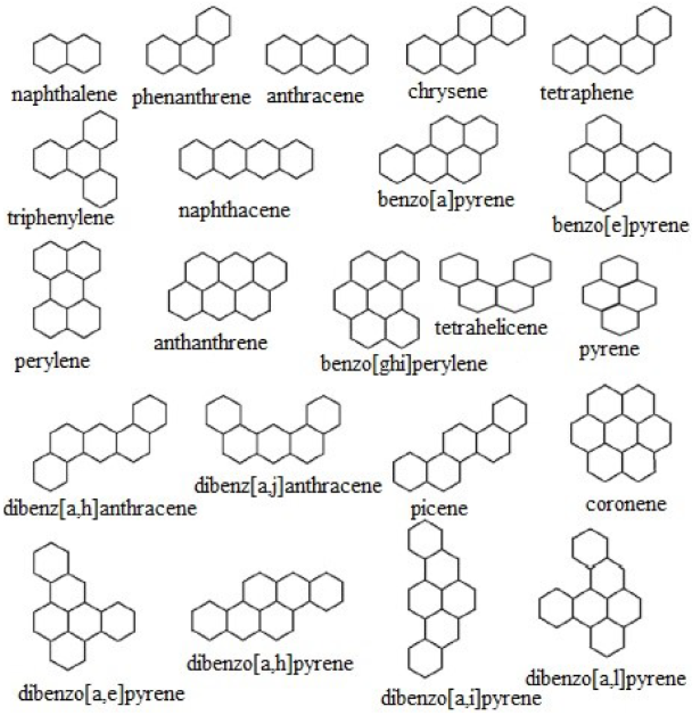
analysis. In order to predict the validity of these new versions of locating indices we consider one branch of Benzene which is the polycyclic aromatic hydrocarbons. For the two other kinds the linear and branched hydrocarbons, whose properties can also be described by these kind of indices, according to the result obtained in this report, we can predict the validities of the new version of locating indices in the other two kind of hydrocarbons. Hence, we leave this investigation for future work. Benzene ( C 6 H 6 ) is an organic chemical compound composed of six carbon atoms joined in a planar ring with one hydrogen atom attached to each ring. Benzene is classified as a hydrocarbon because it contains only hydrogen and carbon atoms. Benzene is a natural ingredient of crude oil and is one of the basic petrochemicals. It is described as an aromatic hydrocarbon due to the cyclic connected pi bonds between the carbon atoms. The abbreviation of it is P h H . Benzene is a colorless and highly flammable liquid. It is used as a precursor to the synthesis of more complex chemical structure, such as cumene and ethylbenzene. The toxicity of benzene limits its use in consumer items despite its popularity as a major industrial chemical [23].
To test the predictive ability of these new indices, we discuss the linear regression analysis of 11 benzenoid hydrocarbons, which are used many times to approach the efficiency of any topological descriptor in quantitative structure property relationships. We inspect the following physicochemical properties: boiling point ( B P ) , molar entropy ( S ) , acentric factor ( ϖ ) , octanol–water partition coefficient ( l o g P ) , complexity ( C ) , and Kovats retention index ( R I ) .

2. New Versions of Locating Indices for Some Known Graphs

In this section, by considering new versions of locating indices, we will determine their values for some special graphs such as complete graph, complete bipartite graph, and cycle, wheel and path graph.
Lemma 1.
Let ς be the complete graph with three or more vertices r. Then
1. 
H M 1 L ( ς ) = 2 r r 1 3 .
2. 
H M 2 L ( ς ) = r r 1 r 2 2 2 .
3. 
R L ( ς ) = r r 1 2 r 2 .
4. 
S O L ( ς ) = r r 1 3 2 .
Proof. 
 
  • Let ς be the complete graph with number of vertices r 3 for each vertex v i V ( ς ) let v i is the locating vector associated with it. Then v i = a 1 , a 2 , , a r such that a i = 0 and all the other components equal to 1. Hence | v i + v j | 2 = 2 + 2 r 2 2 = 4 r 1 2 . However, the total number of edges in ς is r r 1 2 and so H M 1 L ( ς ) = 2 r r 1 3 .
  • For any arbitrary locating vectors v i and v j , where i j , we gain v i · v j = r 2 . Therefore H M 2 L ( ς ) = r r 1 r 2 2 2 .
  • For any arbitrary locating vectors v i and v j , where i j , we gain v i · v j = r 2 . Therefore 1 v i · v j = 1 r 2 hence R L ( ς ) = r r 1 2 r 2 of the summation over all edges.
  • For each v i = a 1 , a 2 , , a r we have | v i | 2 = r 1 and hence | v i | 2 + | v j | 2 = 2 ( r 1 ) . Therefore S O L ( ς ) = r r 1 3 2 .
Theorem 1.
Let ς be the complete bipartite graph K r , s , where 1 < r s . Then
1. 
H M 1 L ( ς ) = r s ( 9 ( r + s 2 ) + 2 ) .
2. 
H M 2 L ( ς ) = 4 r s ( r + s 2 ) 2 .
3. 
R L ( ς ) = r s 2 ( r + s 2 ) .
4. 
S O L ( ς ) = r s 5 ( r + s ) 8 .
Proof. 
Let ς be the complete bipartite graph K r , s , where 1 < r s , with two bipartite sets R and S such that | R | = r and | S | = s , by labelling the vertices of ς as V ς = { v 1 , , v r , u 1 , , u s } . It is clear that the corresponding locating v i of the vertex v i has one zero value in the i th position, ( r 1 ) components of value 2, and s components of value 1 for all i = 1 , 2 , , r and the locating vector u j correspond to the vertex u j for all j = 1 , 2 , , s has one zero value in the j th position, ( s 1 ) components of value 2, and r components of value 1. Therefore
  • For any two adjacent vertices v i and u j where i = 1 , 2 , , r and j = 1 , 2 , , s the locating vector v i + u j has ( r 1 ) components of value three, ( s 1 ) components of value three, and two components of value one. Hence, | v i + u j | 2 = 9 ( r 1 ) + 9 ( s 1 ) + 2 = 9 ( r + s 2 ) + 2 for any two adjacent vertices in the two partition sets R and S. Hence, H M 1 L ( ς ) = r s ( 9 ( r + s 2 ) + 2 ) .
  • For any two locating vertices v i and u j corresponding two the adjacent vertices v i and u j in K r , s we have v i · u j = 2 ( r + s 2 ) Hence H M 2 L ( ς ) = 4 r s ( r + s 2 ) 2 .
  • By part 2 we deduce that R L ( ς ) = r s 2 ( r + s 2 ) .
  • For any i = 1 , 2 , , r we have | v i | 2 = 4 r 1 + s and | u j | 2 = 4 s 1 + r for all j = 1 , 2 , , s hence | v i | 2 + | u j | 2 = 5 r + 5 s 8 . Hence S O L ( ς ) = r s 5 ( r + s ) 8 .
Theorem 2.
Let ς be wheel graph W r with r + 1 vertices such that ( r 4 ) . Then
1. 
H M 1 L ( ς ) =   r 4 r 6 2 + 9 r r 1 2 .
2. 
H M 2 L ( ς ) = r [ 4 r 11 2 + 2 r 4 2 ] .
3. 
R L ( ς ) = 2 r 4 r 11 2 r 4 .
4. 
S O L ( ς ) = r 17 r 2 72 r + 81 9 2 r + 4 2 r 2 .
Proof. 
Let ς W r with r + 1 vertices. Suppose that the vertices v 1 , v 2 , , v r , v r + 1 V ς are labeling in the counterclockwise direction and the center of the wheel is labeled v r + 1 . Hence the locating vector v i for each vertex v i where i = 1 , 2 , , r has 0 component in the i th position, three components of value one, and ( r 3 ) components of value two. Where the locating vector v r + 1 that corresponds to the vertex v r + 1 is equal to ( 1 , 1 , , 1 r times , 0 ) . It is straightforward to notice that the permutation components in each vector v i where i = 1 , 2 , , r , is 1 , 0 , 1 . Therefore
  • For any two adjacent vertices v i + v j where i , j { 1 , 2 , , r } , v i + v j vector has two components of value one, two components of value three, one component of value two, and r 4 components of value four. For any vertex v i , where i = 1 , , r we have v i + v r + 1 is a vector contains two components of value one, two components of value two, and ( r 3 ) components of value three. So
    | v i + v j | 2 = 9 ( r 1 ) 2 for i { 1 , 2 , , r } j = r + 1 4 r 6 2 for i , j { 1 , 2 , , r }
    Hence H M 1 L ( ς ) = r 4 r 6 2 + 9 r r 1 2 .
  • Keeping in mind the permutation of components 1 , 0 , 1 in each vector v i where i = 1 , , r . It is clear that for v i and v j any two adjacent vertices where i , j { 1 , 2 , , r } , hence v i · v j 2 = 4 r 11 2 and v i · v r + 1 2 = 2 r 4 2 . Therefore
    H M 2 L ( ς ) = v i v j E ( ς ) 4 r 11 2 + v i v r + 1 E ( ς ) 2 r 4 2 = r [ 4 r 11 2 + 2 r 4 2 ] .
  • From part 2 we deduce that R L ( ς ) = 2 r 4 r 11 2 r 4 .
  • | v i | 2 = 4 r 9 2 for each corresponding locating vector v i with the vertex v i ( i = 1 , 2 , , r ) and | v r + 1 | 2 = r 2 . Hence
    S O L ( ς ) = v i v j E ( ς ) 2 4 r 9 2 + v i v r + 1 E ( ς ) r 2 + 4 r 9 2 = r ( 2 4 r 9 + r 2 + 4 r 9 2 ) = r 17 r 2 72 r + 81 9 2 r + 4 2 r 2 .
    Hence the result.
Theorem 3.
For any path P r where ( r 3 ) . Then
1. 
H M 1 L ( ς ) = 1 3 r r 1 2 r 2 2 r 1 .
2. 
H M 2 L ( ς ) = 1 15 r r 1 r 2 r + 1 r 2 r 1 .
3. 
R L ( ς ) = i = 1 r 1 3 3 i 2 r 3 i r 2 + r 3 r .
4. 
S O L ( ς ) = i = 1 r 1 k = 1 r i k 2 + k = 1 i k 1 2 + k = 1 r i 1 k 2 + k = 1 i + 1 k 1 2 .
Proof. 
Assume that P r is the path with vertices ( r 3 ) . Suppose that the locating function is constructed by identify the vertices as v 1 , v 2 , , v r from left to right. Hence the corresponding vector for each vertex v i V ( ς ) ( i = 1 , , r ) are given as in the following:
v 1 = 0 , 1 , 2 , 3 , , r 1 , v 2 = 1 , 0 , 1 , 2 , , r 2 v r 1 = r 2 , r 3 , , 0 , 1 , v r = r 1 , r 2 , r 3 , , 0 .
By notice the symmetry between the components of the vectors v 1 and v r and v 2 and v r 1 ,....so on. Hence
  • For any two adjacent vertices v i and v i + 1 we have | v i + v i + 1 | 2 = k = 1 r i 2 k 1 2 + k = 1 i   2 k 1 2 where i = 2 , , r 1 . Hence
    H M 1 L ( ς ) = i = 1 r 1 k = 1 r i 2 k 1 2 + i = 1 r 1 k = 1 i 2 k 1 2 = 2 r 4 4 r 3 + r 2 + r 3 .
  • For the other case H M 2 L ( ς ) we have v i · v i + 1 = k = 1 r i k k 1 + k = 1 i k k 1 , hence
    H M 2 L ( ς ) = i = 1 r 1 v i · v i + 1 2 = i = 1 r 1 k = 1 r i k k 1 2 + i = 1 r 1 k = 1 i k k 1 2 = 1 6 r 3 1 30 r 2 1 15 r 1 10 r 5 + 1 30 r 6 1 30 r r 1 r + 1 r 2 r 2 + r + 1 = 1 15 r r 1 r 2 r + 1 r + r 2 1 .
    Therefore, H M 2 L ( ς ) is obtained as required in the statement of theorem.
  • From part 2, we have
    R L ( ς ) = i = 1 r 1 1 k = 1 r i k k 1 + k = 1 i k k 1 = i = 1 r 1 1 3 r i 2 3 r 2 i + r 3 r 3 = i = 1 r 1 3 3 i 2 r 3 i r 2 + r 3 r .
  • With some calculation we conclude that | v i | 2 = k = 1 r i k 2 + k = 1 i k 1 2 and | v i + 1 | 2 = k = 1 r i 1 k 2 + k = 1 i + 1 k 1 2 . Hence
    S O L ( ς ) = i = 1 r 1 k = 1 r i k 2 + k = 1 i k 1 2 + k = 1 r i 1 k 2 + k = 1 i + 1 k 1 2 .
    Which is the required result.
Theorem 4.
For an even integer r 4 , let ς C r . Then
1. 
H M 1 L ( ς ) = r 2 1 r 2 + 1 3 .
2. 
H M 2 L ( ς ) = r r 3 4 r 2 144 .
3. 
R L ( ς ) = 2 r r 3 4 r 3 .
4. 
S O L ( ς ) = r 1 3 r + 1 6 r 3 .
Proof. 
By identifying the vertices of the cycle C r as v 1 , v 2 , , v r in the counterclockwise direction. Then the locating vector v i correspond to the vertex v i has zero component in the position i , one component of value r 2 1 , two components of values of value 1, two components of value 2, and two components of value 3. Hence, for any two adjacent vertices v i and v i + 1 where i = 1 , 2 , , r 1
  • For any two adjacent vertices v i and v i + 1 we have | v i + v i + 1 | 2 = 2 k = 1 r 2 2 k 1 2 . Therefore
    H M 1 L ( ς ) = 2 r k = 1 r 2 2 k 1 2 = r r 3 r 3 = r 4 r 3 3 = r 2 1 r 2 + 1 3 .
  • we have v i · v i + 1 = 2 i = 2 r 2 i i 1 = 1 12 r 3 1 3 r . Therefore H M 2 L ( ς ) = r 2 i = 2 r 2 i i 1 2 = r r 3 4 r 2 144 .
  • By part 2, R L ( ς ) = r 2 i = 2 r 2 i i 1 1 2 = 2 r r 3 4 r 3 .
  • We can see that each v i has equivalent components but in different location, hence each | v i | 2 has the same sum as the form of
    | v i | 2 = r r + 1 r + 2 3 r 2 12 .
    Hence
    S O L ( ς ) = v i v j E ( ς ) | v i | 2 + | v j | 2 = r r r + 1 r + 2 3 r 2 12 + r r + 1 r + 2 3 r 2 12 = r 1 3 r + 1 6 r 3 .
Theorem 5.
For an odd integer r 3 , let ς C r . Then
1. 
H M 1 L ( ς ) = r 2 r 3 3 r 2 2 r + 15 6 .
2. 
H M 2 L ( ς ) = 1 12 r + 3 r 1 r 2 .
3. 
R L ( ς ) = 2 3 r r 1 r 2 r + 3 .
4. 
S O L ( ς ) = r 1 6 r r 2 1 .
Proof. 
We notice the following vectors in the cycle C r
v 1 = 0 , 1 , 2 , 3 , , r 1 2 , r 1 2 1 , r 1 2 2 , , 1 , v 2 = 1 , 0 , 1 , 2 , , r 1 2 1 , r 1 2 , r 1 2 1 , , 2 , v 3 = 2 , 1 , 0 , 1 , , r 1 2 2 , r 1 2 1 , r 1 2 , , 3 , v r = 1 , 2 , 3 , , r 1 2 , r 1 2 1 , r 1 2 2 , , 0 .
with some calculation we obtain
  • For any two adjacent vertices v i and v i + 1 we have | v i + v i + 1 | 2 = 2 k = 1 r 1 2 2 k 1 2 + 2 r 1 2 2 = 1 3 r 3 1 2 r 2 1 3 r + 1 2 , hence
    H M 1 L ( ς ) = r 2 r 3 3 r 2 2 r + 15 6 .
  • Additionally,
    v i · v i + 1 = 2 i = 1 r 1 2 i i 1 + r 1 2 4 = 2 r 1 2 r 1 2 + 1 2 r 1 2 + 1 6 1 2 r 1 2 r 1 2 + 1 2 1 + r 1 2 4 = 1 12 r 3 7 12 r + 1 2 = 1 12 r + 3 r 1 r 2 .
    Hence H M 2 L ( ς ) = 1 12 r + 3 r 1 r 2 as required.
  • By part 2, R L ( ς ) = 2 3 r r 1 r 2 r + 3 .
  • For S O L ( ς ) we have | v i | 2 = 2 i = 1 r 1 2 i 2 = r r 2 1 12 which implies
    S O L ( ς ) = r r r 2 1 12 + r r 2 1 12 = r 1 6 r r 2 1 .

3. New Versions of Locating Indices and Helm Graph

In this Section we will compute the exact value of new versions of locating indices of the Helm graph. Recall that [24] Helm graph ( H r ) is a simple graph obtained from the r - wheel W m graph next to the edge of the pendant at each vertex of the C r cycle.
Theorem 6.
Given that H r be a helm graph with r 3 . Then
1. 
H M 1 L ( ς ) = r 212 r 431 2 .
2. 
H M 2 L ( ς ) = r 15 r 49 2 + r 18 r 36 2 + r 8 r 14 2 .
3. 
R L ( ς ) = r 15 r 49 + 18 r 36 + 8 r 14 .
4. 
S O L ( ς ) = 2 r 13 r 27 + r 13 r 27 2 + 15 r 14 2 + r 13 r 27 2 + 25 r 2 .
Proof. 
Let H r be the Helm graph obtained by attaching a pendant edge at each vertex of the cycle. Let V ( H r ) = { v 0 } { v 1 , v 2 , , v r } { v r + 1 , v r + 2 , , v 2 r } where v i s are the vertices of cycles taken in cyclic order and v r + i s are pendant vertices such that each v i v r + i is a pendant edge and v 0 is the center of the cycle. Therefore, we obtain the corresponding vectors v i for each vertex v i V ( H r ) where i = 1 , 2 , , r as follows:
v 1 = 0 , 1 , 2 , , 2 r 3 , 1 , 1 , 2 , 3 , , 3 r 3 , 2 , 1 , v 2 = 1 , 0 , 1 , 2 , , 2 r 2 , 1 , 2 , 3 , , 3 r 3 , 1 , , , v r = 1 , 2 , , 2 r 3 , 1 , 0 , 2 , 3 , , 3 r 3 , 2 , 1 , 1
Hence, each v i = 0 i t h p o s i t i o n , 2 , , 2 r 1 , 1 , , 1 4 t i m e s , 3 , , 3 r 3 , more clearly has 0 component in i th position, ( r 1 ) components of value two, r 3 components of value three, and four comonents of value one. Moreover, the corresponding vectors v r + i for each vertex v r + i V ( H r ) where i = 1 , 2 , , r as follows:
v r + 1 = 1 , 2 , 3 , 3 r 3 , 2 , 0 r + 1 position , 3 , 4 , 4 r 3 , 3 , 2 , v r + 2 = 2 , 1 , 2 , 3 , , 3 r 2 , 0 r + 2 position , 3 , 4 , 4 r 3 , 2 , , , v 2 r = 2 , 3 , 3 r 3 , 2 , 1 , 3 , 4 , 4 r 3 , 3 , 0 2 r position , 2
Hence, each v r + i = 0 ( r + i ) t h p o s i t i o n , 2 , , 2 3 t i m e s , 1 r t h p o s i t i o n , 3 , , 3 r 1 , 4 , , 4 r 3 , more clearly has 0 component in r + i t h position, ( r 1 ) components of value three, r 3 components of value four, and three competent of value two. Finally the corresponding vectors v 0 for each vertex v 0 V ( H r ) is v 0 = 1 , , 1 r times , 2 , , 2 r times , 0 . Now let A , B , C V ( H r ) such that
A = { v 1 , v 2 , , v r } , B = { v r + 1 , v r + 2 , , v 2 r } , and C = { v 0 } .
Hence,
  • H M 1 L ( ς ) = v i , v i + 1 A v i v i + 1 | v i + v i + 1 | 2 ( 1 ) + v i , A , v r + i B v i v r + i | v i + v r + i | 2 ( 2 ) + v i A , v 0 C v i v 0 | v i + v 0 | 2 ( 3 ) . For the summation (1), we have
    v 1 + v 2 = 1 , 1 , 3 , 4 , , 4 r 4 , 3 , 3 , 3 , 5 , 6 , , 6 r 4 , 5 , 2 , v 2 + v 3 = 3 , 1 , 1 , 3 , 4 , , 4 r 4 , 5 , 3 , 3 , 5 , 6 , , 6 r 4 , 2 , , v r 1 + v r = 3 , 4 , , 4 r 4 , 3 , 1 , 1 , 5 , 6 , , 6 r 4 , 5 , 3 , 3 , 2 v 1 + v r = 1 , 3 , 4 , , 4 r 4 , 3 , 1 , 2 , 5 , 6 , , 6 r 4 , 5 , 3 , 2
    Hence, each v i + v i + 1 = 1 2 t i m e s , 2 1 t i m e s , 3 , , 3 4 t i m e s , 4 , , 4 r 4 , 5 2 t i m e s , 6 , , 6 r 4 , more clearly has 1 two times, 2 one time, 3 four times, ( r 4 ) components of value four, r 4 components of value six, and 5 two times. Also v 1 + v r = 1 2 t i m e s , 2 2 t i m e s , 3 , , 3 3 t i m e s , 4 , , 4 r 4 , 5 2 t i m e s , 6 , , 6 r 4 , more clearly has 1 two times, 2 two times, 3 three times, ( r 4 ) components of value four, r 4 components of value six, and 5 two times. Therefore
    v i , v i + 1 A v i v i + 1 | v i + v i + 1 | 2 = v i , v i + 1 A v i v i + 1 179 + 104 r 416 2 = r 104 r 237 2 .
    For summation in (2), we have
    v 1 + v r + 1 = 1 , 3 , 5 , , 5 r 2 , 3 , 1 , 5 , 7 , , 7 r 3 , 5 , 3 , v 2 + v r + 2 = 3 , 1 , 3 , 5 , , 5 r 2 , 15 , 7 , , 7 r 3 , 3 , , v r + v 2 r = 3 , 5 , , 5 r 3 , 3 , 1 , 5 , 7 , , 7 r 3 , 5 , 1 , 3
    Hence each v i + v r + i = 1 2 t i m e s , 3 , , 3 3 t i m e s , 5 r 1 , 7 , , 7 r 3 , more clearly has 1 two times, 3 three times, r 1 components of value five, and r 3 competent of value seven. Therefore
    v i , A , v r + i B v i v r + i | v i + v r + i | 2 = v i , A , v r + i B v i v r + i 74 r 143 2 = r 74 r 143 2 .
    For summation in (3)
    v 1 + v 0 = 1 , 2 , 3 , , 3 r 1 , 2 , 3 , 4 , 5 , , 5 r 3 , 4 , 1 , v 2 + v 0 = 1 , 2 , 3 , , 3 r 1 , 2 , 3 , 4 , 5 , , 5 r 3 , 4 , 1 , , v r + v 0 = 2 , 3 , , 3 r 1 , 2 , 1 , 4 , 5 , , 5 r 3 , 4 , 3 , 1
    Hence, each v i + v 0 = 1 2 t i m e s , 2 2 t i m e s , 3 , , 3 r 2 , 4 2 t i m e s , 5 , , 5 r 3 , more clearly has 1 two times, 2 two times, r 2 components of value three, 2 times of value 4, and r 3 competent of value five. Therefore v i A , v 0 C v i v 0 | v i + v 0 | 2 = v i A , v 0 C v i v 0 34 r 51 2 = r 34 r 51 2 . Hence
    H M 1 L ( ς ) = r 104 r 237 2 + 74 r 143 2 + 34 r 51 2 = r 212 r 431 2 .
  • H M 2 L ( ς ) = v i , v i + 1 A v i v i + 1 v i · v i + 1 2 ( 1 ) + v i , A , v r + i B v i v r + i v i · v r + i 2 ( 2 ) + v i A , v 0 C v i v 0 v i · v 0 2 ( 3 ) . For summation (1), we have v i , v i + 1 A v i v i + 1 v i · v i + 1 2 = r 4 r 4 + 2 ( r 5 ) + 9 ( r 4 ) + 13 2 = r 15 r 49 2 . For summation (2), we have v i , A , v r + i B v i v r + i v i · v r + i 2 = r [ 6 r 1 +
    12 r 3 + 6 ] 2 = r 18 r 36 2 . For summation (3), we have v i A , v 0 C v i v 0 v i · v 0 2 = r 6 r 3 + 2 r 3 + 10 2 = r 8 r 14 2 . Hence H M 2 L ( ς ) = r 15 r 49 2 + r 18 r 36 2 + r 8 r 14 2 .
  • It is clear from part 2 that R L ( ς ) = r 15 r 49 + 18 r 36 + 8 r 14 .
  • S O L ( ς ) = v i , v i + 1 A v i v i + 1 | v i | 2 + | v i + 1 | 2 ( 1 ) + v i , A , v r + i B v i v r + i | v i | 2 + | v r + i | 2 ( 2 ) + v i A , v 0 C v i v 0 | v i | 2 + | v 0 | 2 ( 3 ) . For summation in (1)
    v i , v i + 1 A v i v i + 1 | v i | 2 + | v i + 1 | 2 = r 2 4 r 1 + 9 ( r 3 + 4 ) 2 = r 2 13 r 27 2 = 2 r 13 r 27 .
    For summation in (2)
    v i , A , v r + i B v i v r + i | v i | 2 + | v r + i | 2 = r 4 r 1 + 9 ( r 3 + 4 ) 2 + 9 r 1 + 6 r 3 + 13 2 = r 13 r 27 2 + 15 r 14 2
    For summation in (3)
    v i A , v 0 C v i v 0 | v i | 2 + | v 0 | 2 = r 13 r 27 2 + 25 r 2 .
    Hence, S O L ( ς ) = 2 r 13 r 27 + r 13 r 27 2 + 15 r 14 2 + r 13 r 27 2 + 25 r 2 .

4. Significance of New Versions of Locating Indices

Accordant to Milan Randić [25] in order to consider a topological index as an acceptable index, it must satisfy some of the following conditions: have positive correlation with at least one property; have structural interpretation; preferably contradistinguish; be generalizable to more advanced analogues; be elementary; not be established based on properties; not be trivially related to other descriptors; be possible to compose effectively; and be based on organizable structural abstractions. In this section, we considered 11 benzenoid hydrocarbons to test the anticipating capability of these new indices. The experimental data of 11 benzenoid hydrocarbons are found in references [26,27,28], and also https://pubchem.ncbi.nlm.nih.gov (accessed on 26 March 2022). Table 1 indicates the experimental data of benzenoid hydrocarbons. Table 2 shows the new index-values of benzenoid hydrocarbons. Molecular graphs of benzenoid hydrocarbons are depicted in Figure 1. We have seen that these indices play a crucial part in evaluation the boiling point ( B P ) , molar entropy ( S ) , acentric factor ( ϖ ) , octanol–water partition coefficient ( l o g P ) , complexity ( C ) , and Kovats retention index ( R I ) of these 11 benzenoid hydrocarbons. Table 3 shows the correlation coefficient (R) of the these indices with some physicochemical properties of 11 benzenoid hydrocarbons (where the significance of bold numbers denote highest correlation value).

4.1. Regression Model

Using the data in Table 1 and Table 2, linear regression models were obtained for boiling point ( B P ) , molar entropy ( S ) , acentric factor ( ϖ ) , octanol–water partition coefficient ( l o g P ) , complexity ( C ) , and Kovats retention index ( R I ) . The corresponding R were calculated. Where, N , R 2 , S e , F , and S F denote the population, coefficient of determination, standard error of estimate, Fischer F-values, F-significance, respectively. We have tested the following linear regression model P = A + B ( L I ) where P = physical property, L I = locating index. We have obtained the following different linear models for each of the locating indices, which are listed below:
(1)
First Hyper Locating Index H M 1 L ( ς ) :
B P = 235.916 + 0.01 [ H M 1 L ( ς ) ]
ϖ = 0.312 + 7.1 × 10 ( 6 ) [ H M 1 L ( ς ) ]
L o g P = 3.31 + 1.1 × 10 ( 4 ) [ H M 1 L ( ς ) ]
R I = 206.488 + 0.009 [ H M 1 L ( ς ) ]
C = 136.682 + 0.007 [ H M 1 L ( ς ) ]
S = 80.340 + 0.001 [ H M 1 L ( ς ) ]
(2)
Second Hyper Locating Index H M 2 L ( ς ) :
B P = 296.857 + 9.8 × 10 ( 5 ) [ H M 2 L ( ς ) ]
ϖ = 0.354 + 7.28 × 10 ( 8 ) [ H M 2 L ( ς ) ]
L o g P = 3.991 + 1.2 × 10 ( 6 ) [ H M 2 L ( ς ) ]
R I = 263.502 + 9.6 × 10 ( 5 ) [ H M 2 L ( ς ) ]
C = 180.186 + 6.9 × 10 ( 5 ) [ H M 2 L ( ς ) ]
S = 87.27 + 1.24 × 10 ( 5 ) [ H M 2 L ( ς ) ]
(3)
Randić Locating Index R L ( ς ) :
B P = 278.037 + 95.673 [ R L ( ς ) ]
ϖ = 0.602 0.115 [ R L ( ς ) ]
L o g P = 5.638 0.126 [ R L ( ς ) ]
R I = 321.911 + 41.301 [ R L ( ς ) ]
C = 180.445 + 57.871 [ R L ( ς ) ]
S = 114.458 8.049 [ R L ( ς ) ]
(4)
Sombor Locating Index S O L ( ς ) :
B P = 210.599 + 0.524 [ S O L ( ς ) ]
ϖ = 0.293 + 0.00039 [ S O L ( ς ) ]
L o g P = 3.105 + 0.006 [ S O L ( ς ) ]
R I = 186.921 + 0.493 [ S O L ( ς ) ]
C = 101.352 + 0.414 [ S O L ( ς ) ]
S = 78.212 + 0.061 [ S O L ( ς ) ]

4.2. Results and Discussion

Using the regression models, we calculated the correlation coefficients ( R ) between versions of new locating indices and some physiochemical properties of benzenoid hydrocarbons shown in Table 3. Scatter plots between the boiling point ( B P ), molar entropy ( S ) , acentric factor ( ϖ ) , octanol–water partition coefficient ( l o g P ) , and Kovats retention index ( R I ) with new locating indices are shown in Figure 2.

4.3. Concluding Remarks

By analyzing the data given in Table 4, Table 5, Table 6 and Table 7, it is possible to derive some results for the given new locating indices (expect for the Randić locating index which will be excluded from our discussion). These tables show the regression model of various physicochemical properties. It can be observed that the regression model value R is more than 0.6 and significance F is less than 0.05 . Hence, it can be observed that all the physical and chemical properties of benzenoid hydrocarbons are positively correlated with the defined new locating indices. First, the Randić locating index was found to be completely inadequate for any structure–property correlation, although many models have been tested to validate this index it did not pass these tests. Second, the Sombor locating index, Table 7, depicts that this index is a beneficial tool in deriving the physical and chemical properties for benzenoid hydrocarbons with correlation coefficient values lying between 0.972 to 0.982 except for the complexity of benzenoid hydrocarbons, where the correlation coefficient value of the Sombor locating index with complexity is 0.788 . More clearly, when examining the table correlation coefficients horizontally for physical properties, we see that S O L ( ς ) index gives highest correlation coefficient for boiling point ( B P ) ( R = 0.980 ), molar entropy ( S ) ( R = 0.975 ), acentric factor ( ϖ ) ( R = 0.972 ) , octanol–water partition coefficient ( l o g P ) ( R = 0.978 ) , complexity ( C ) ( R = 0.788 ) , and Kovats retention index ( R I ) ( R = 0.982 ) . Sombor locating index is highly recommended for predicting the Q S P R of benzenoid hydrocarbons. The first Hyper locating index shows good correlation properties. The Q S P R study in Table 4 shows that the predicting power of this index is quite satisfactory, with range of 0.930 R 0.967 , excluding the complexity value of 0.669 . On the other hand, the second Hyper locating index has a positive and highly significant correlation coefficient for molar entropy ( S ) ( R = 0.905 ) and for others, and for the physical and chemical properties for benzenoid hydrocarbons, the range of the correlation coefficient is between 0.843 and 0.894 .
In this paper, we introduce four new versions of locating indices, and find their exact values for some families of known graphs and for the Helm graph. We examined the efficiency of predicting the physicochemical properties of benzenoid hydrocarbons. Raw data from the chemistry literature and a mathematical effort to find new topological indices are joined in this study to introduce these novel indices which will encourage its utilization prospects in pharmacological and chemical fields. The cases in which satisfactory correlations were gained proposed the effectiveness of the computed topological indices to be useful in predicting the physicochemical properties of numerous intricate chemical compounds. For instance, they can be used in the characterization of nanotubes and graphene structures. This study predicted the validity new versions of locating indices. They have been applied for a series of polycyclic aromatic hydrocarbons. The study is reliable since it tested eleven polycyclic aromatic hydrocarbons. Accordingly, we can suggest applying these new indices to other types of compounds such as the linear and branched alkanes.

4.4. Comparative Analysis

To grasp the significance of these new indices, we will compare the results obtained from the new versions of locating indices and some known indices in the literature. The efficiency and applicability measured by comparable correlation coefficient (R) of the new versions of locating indices and those of other known indices is shown in Table 8. The R values of each index are very similar, range from 0.972 to 0.980. The unavailable data in the table inspires more questions for future investigation to compare different topological indices with our calculations of the new locating indices and to conduct more research into the different types of benzenoid hydrocarbons.

Author Contributions

Conceptualization, S.W. and A.S.; methodology, S.W.; software, S.W.; validation, S.W. and A.S.; formal analysis, S.W. and A.S.; investigation, S.W.; resources, S.W.; data curation, A.S.; writing—original draft preparation, S.W.; writing—review and editing, S.W.; visualization, S.W. and A.S.; supervision, A.S.; project administration, A.S.; funding acquisition, S.W. All authors have read and agreed to the published version of the manuscript.

Funding

This work was funded by the Deanship of Scientific Research (DSR), King Abdulaziz University, Jeddah, under grant No (D-461-247-1443).

Institutional Review Board Statement

Not applicable.

Informed Consent Statement

Not applicable.

Data Availability Statement

The physical property data used to support the findings of this study are included within the article.

Acknowledgments

We are extremely obligated to the referees, whose valuable suggestions led us to improve the manuscript. The authors acknowledge with thanks DSR’s technical and financial support.

Conflicts of Interest

The authors declare that they have no conflict of interest to report regarding the present study.

References

  1. Gutman, I.; Polansky, O.E. Mathematical Concepts in Organic Chemistry; Springer: Berlin, Germany, 1986. [Google Scholar]
  2. Bindusree, A.R.; Cangul, I.N.; Lokesha, V.; Çevik, A.S. Zagreb polynomials of three graph operators. Filomat 2016, 30, 1979–1986. [Google Scholar] [CrossRef] [Green Version]
  3. John, P.E.; Khadikar, P.V.; Singh, J. A method of computing the PI index of benzenoid hydrocarbons using orthogonal cuts. J. Mathematical Chem. 2007, 42, 37–45. [Google Scholar] [CrossRef] [Green Version]
  4. Nikolić, S.; Milixcxevixcx, A.; Trinajstixcx, N. QSPR study of polarographic half-wave reduction potentials of benzenoid hydrocarbons. Croat. Chem. Acta 2006, 79, 155–159. [Google Scholar]
  5. Özalan, N.U. Some Indices over a New Algebraic Graph. J. Math. 2021, 2021, 5510384. [Google Scholar] [CrossRef]
  6. Wagner, S.G. A Class of trees and its Wiener index. Acta Appl. Math. 2006, 91, 119–132. [Google Scholar] [CrossRef] [Green Version]
  7. Wang, H.; Yu, G. All but 49 numbers are Wiener indices of trees. Acta Appl. Math. 2006, 92, 15–20. [Google Scholar] [CrossRef]
  8. Ananda, N.; Ranjini, P.S.; Lokesha, V.; Wazzan, S.A. Subdivision and semi total point graphs of Archimedean lattices on some topological indices. Proc. Jangjeon Math. Soc. 2020, 22, 583–592. [Google Scholar]
  9. Wazzan, S.A. Some New Topological Indices of Aspirin. Proc. Jangjeon Math. Soc. 2020, 23, 113–124. [Google Scholar]
  10. Wazzan, S.A. Topological Indices of Parkinson’s Disease Drug Carbidopa. Far East J. Math. Sci. 2019, 118, 1. [Google Scholar] [CrossRef]
  11. Gutman, I.; Togan, M.; Yurttas, A.; Çevik, A.S.; Cangul, I.N. Inverse problem for sigma index, MATCH Commun. Math. Comput. Chem. 2018, 79, 491–508. [Google Scholar]
  12. Gutman, I.; Yeh, Y. The sum of all distances in bipartite graphs. Math. Slovaca 1995, 45, 327–334. [Google Scholar]
  13. Ranjini, P.S.; Lokesha, V.; Çevik, A.S.; Cangul, I.N. Sharp bounds for SZ, PI and GA_2 indices in terms of the number of triangles. Ilir. J. Math. 2015, 4, 41–49. [Google Scholar]
  14. Lokesha, V.; Suvarna, S.; Çevik, A.S.; Cangul, I.N. VL Reciprocal status index and co-index of graphs. J. Math. 2021, 2021, 5529080. [Google Scholar] [CrossRef]
  15. Das, K.C.; Çevik, A.S.; Cangul, I.N.; Shang, Y. On Sombor index. Symmetry 2021, 13, 140. [Google Scholar] [CrossRef]
  16. Demirci, M.; Delen, S.; Çevik, A.S.; Cangul, I.N. Omega index of line and total graphs. J. Math. 2021, 2021, 5552202. [Google Scholar] [CrossRef]
  17. Wazzan, S.; Saleh, A. On the First and Second Locating Zagreb Indices of Graphs. Appl. Math. 2019, 10, 805–816. [Google Scholar]
  18. Wazzan, S.; Saleh, A. Locating and Multiplicative Locating Indices of Graphs with QSPR Analysis, Hindawi. J. Math. 2021, 2021, 5516321. [Google Scholar] [CrossRef]
  19. Shirdel, G.H.; Rezapour, H.; Sayadi, A.M. The hyper Zagreb index of graph operations. Iran. J. Math. Chem. 2013, 4, 213–220. [Google Scholar]
  20. Randić, M. On characterization of molecular branching. J. Am. Chem. Soc. 1975, 97, 6609–6615. [Google Scholar] [CrossRef]
  21. Gutman, I. Geometric approach to degree-based topological indices: Sombor indices. MATCH Commun. Math. Comput. Chem. 2021, 86, 11–16. [Google Scholar]
  22. Ramaswamy, H.N.; Alwardi, A.; Kumar, N.R. On the locating matrix of a graph and its spectral analysis. Comp. Scien. J. Moldova 2017, 25, 75. [Google Scholar]
  23. Dias, J.R. Handbook of Polycyclic Hydrocarbons. Part A: Benzenoid Hydrocarbons; Elsevier Science Ltd.: Amsterdam, The Netherlands, 1987. [Google Scholar]
  24. Hayyu, A.N.; Dafik, I.M.; Tirta, R.; Adawiyah, R.M. Prihandini, Resolving domination number of helm graph and it’s operation. J. Phys. Conf. Ser. 2020, 1465, 012022. [Google Scholar] [CrossRef]
  25. Randić, M. Generalized molecular descriptors. J. Math. Chem. 1991, 7, 155–168. [Google Scholar] [CrossRef]
  26. Alberty, R.A.; Reif, A.K. Standard chemical thermodynamic properties of polycyclic aromatic hydrocarbons and their isomer groups I. Benzene series. J. Phys. Chem. Ref. Data 1988, 17, 241–253, Erratum in J. Phys. Chem. Ref. Data 1989, 18, 551–553. [Google Scholar] [CrossRef] [Green Version]
  27. Wang, H.; Frenklach, M. Transport properties of polycyclic aromatic hydrocarbons for flame modeling. Combust. Flame 1994, 96, 163–170. [Google Scholar] [CrossRef]
  28. White, C.M. Prediction of the boiling point, heat of vaporization, and vapor pressure at various temperatures for polycyclic aromatic hydrocarbons. J. Chem. Eng. Data 1986, 31, 198–203. [Google Scholar] [CrossRef]
  29. Nikolić, S.; Milixcxevixcx, A.; Trinajstixcx, N.; Jurixcx, A. On Use of the Variable Zagreb vM2 Index in QSPR: Boiling Points of Benzenoid Hydrocarbons. Molecules 2004, 9, 1208–1221. [Google Scholar] [CrossRef] [Green Version]
  30. Rachanna, K.; Shigehalli, V. QSPR Analysis of Degree-Based Topological Indices with physical properties of Benzenoid Hydrocarbons. Gen. Lett. Math. 2017, 2, 150–169. [Google Scholar]
  31. Rajasekharaiah, V.G.; Murthy, P.U. Hyper-Zagreb indices of graphs and its applications. J. Algebra Comb. Discret. Appl. 2021, 8, 9–22. [Google Scholar] [CrossRef]
Figure 1. Molecular graphs of benzenoid hydrocarbons.
Symmetry 14 01022 g001
Figure 2. Physicochemical properties of benzoid hydrocarbons with topological indices.
Symmetry 14 01022 g002
Table 1. Experimental values of some physicochemical properties of benzenoid hydrocarbons.
Benzenoid Hydrocarbons ( BP ) ( S ) ( ϖ ) LogP ( RI ) ( C )
naphthalene218 79.38 0.302 3.3 200 80.6
phenanthrene338 93.79 0.39 4.46 300335
chrysene431 106.83 0.46 5.81 400264
tetraphene425 108.22 0.46 5.76 398.5 294
triphenylene429 104.66 0.46 5.49 400217
tetrahelicene436 0.47 5.7 391.12 266
perylene497 109.10 0.49 6.25 456.22 217
naphthacene440 105.47 0.46 5.76 408.3 304
pyrene404 96.06 0.41 4.88 351.22 236
benzo[a]pyrene496 111.85 6.13 453.44 372
benzo[e]pyrene493 110.46 6.44 450.73 336
Table 2. New locating indices of benzenoid hydrocarbons.
Benzenoid Hydrocarbons HM 1 L ( ς ) HM 2 L ( ς ) R L ( ς ) SO L ( ς )
naphthalene2857412,4831.482637.7094
phenanthene8834300,9681.4640261.804
chrysene21,738155,3031.3854474.224
tetraphene22,490165,1331.3583416.911
triphenylene17,963101,0681.5071375.695
tetrahelicene20,446134,9491.4325399.556
naphthacene24,314193,7651.3058429.787
pyrene11,696462,1421.6024328.713
perylene24,699163,1611.5707531.393
benzo[a]pyrene27,576215,7601.4943575.456
benzo[e]pyrene24,158159,4511.5832537.929
Table 3. Correlation coefficients (R) between versions of new locating indices and some physiochemical properties of benzenoid hydrocarbons.
Locating Index BP S ϖ LogP RI C
H M 1 L ( ς ) 0.930 0.967 0.945 0.964 0.955 0.669
H M 2 L ( ς ) 0.843 0.905 0.859 0.894 0.878 0.602
R L ( ς ) 0.112 0.080 0.194 0.013 0.052 0.069
S O L ( ς ) 0 . 980 0 . 975 0 . 972 0 . 978 0 . 982 0 . 788
Table 4. Statical parameters for the linear QSPR model for first Hyper locating index.
Physical PropertiesN R 2 Se F SF
boiling point ( B P ) 11 0.866 31.317 57.973 3 × 10 ( 5 )
molar entropy ( S ) 10 0 . 935 2.729 114.332 5.1 × 10 ( 6 )
octanol partition coefficient ( l o g P ) 11 0.930 0.256 119.359 1.7 × 10 ( 7 )
complexity ( C ) 11 0.447 62.32 7.273 0.025
Kovats retention index ( R I ) 11 0.913 23.7 93.939 4.6 × 10 ( 6 )
acentric factor ( ϖ ) 9 0.892 0.02 57.864 0.0001
Table 5. Statical parameters for the linear QSPR model for second Hyper locating index.
Physical PropertiesN R 2 Se F SF
boiling point ( B P ) 11 0.711 45.928 22.14 0.001
molar entropy ( S ) 10 0 . 819 4.5335 36.295 0.0003
octanol partition coefficient ( l o g P ) 11 0.799 0.433 35.865 0.0002
complexity ( C ) 11 0.771 38.333 30.351 0.0004
Kovats retention index ( R I ) 11 0.362 66.914 5.116 0.05
acentric factor ( ϖ ) 9 0.738 0.032 19.7533 0.003
Table 6. Statical parameters for the linear QSPR model for Randić locating index.
Physical PropertiesN R 2 Se F SF
boiling point ( B P ) 11 0.013 84.890 0.115 0.742
molar entropy ( S ) 10 0.006 10.63802 0.051 0.827
octanol partition coefficient ( l o g P ) 11 0.001 0.96577 0.002 0.970
complexity ( C ) 11 0.005 80.04642 0.024 0.880
Kovats retention index ( R I ) 11 0.003 83.5988 0.043 0.840
acentric factor ( ϖ ) 9 0 . 038 0.061 0.274 0.067
Table 7. Statical parameters for the linear QSPR model for Sombor locating index.
Physical PropertiesN R 2 Se F SF
boiling point ( B P ) 11 0.961 16.879 221.565 1.2 × 10 ( 7 )
molar entropy ( S ) 10 0.950 2.382 152.546 1.7 × 10 ( 6 )
octanol partition coefficient ( l o g P ) 11 0.956 0.203 193.882 2.1 × 10 ( 7 )
complexity ( C ) 11 0.621 51.56 14.775 0.004
Kovats retention index ( R I ) 11 0 . 965 15.003 247.879 7.4 × 10 ( 8 )
acentric factor ( ϖ ) 9 0.945 0.014 120.011 1.1 × 10 ( 5 )
Table 8. Correlation coefficients (R) between some topological indices and the physiochemical properties of benzenoid hydrocarbons.
Topolgical Index BP S ϖ LogP RI C
M 1 ( ς ) [First Zagreb index]
M 2 ( ς ) [Second Zagreb index]0.980 [29]
R ( ς ) [Randić Index]0.975 [30] 0.972 [30]
H ( ς ) [hyper Index]0.974 [31] 0.972 [30]
S O ( ς ) [Sombor index]
Publisher’s Note: MDPI stays neutral with regard to jurisdictional claims in published maps and institutional affiliations.

