Author Contributions
Conceptualization, K.L. and K.N.; methodology, K.L.; software, K.L.; validation, K.N., K.O., R.K. and T.N.; formal analysis, K.N.; investigation, K.O., R.K., and T.N.; resources, K.O.; data curation, K.L. and K.N.; writing—original draft preparation, K.L.; writing—review and editing, K.O. and R.K.; visualization, K.L.; supervision, K.N. and K.O.; project administration, K.N., K.O., R.K. and T.N. All authors have read and agreed to the published version of the manuscript.
Figure 1.
Intracapsular fracture occurring because of low-energy falls in the elderly: (a) CT diagnostic image; (b) 3D reconstruction model.
Figure 1.
Intracapsular fracture occurring because of low-energy falls in the elderly: (a) CT diagnostic image; (b) 3D reconstruction model.
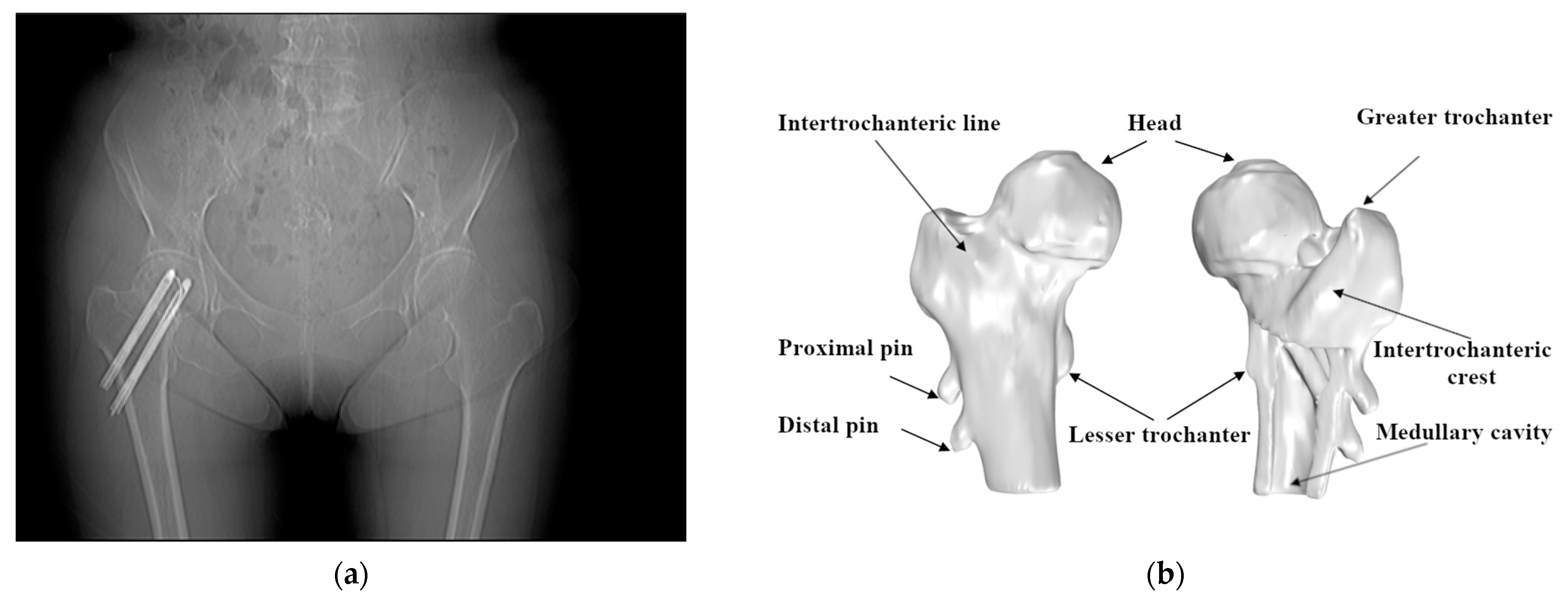
Figure 2.
Use of the Hansson pin for the fixation of femoral neck fractures: (a) the anteroposterior/posteroanterior X-ray (AP X-ray) of intracapsular fracture fixation using two Hansson pins; (b) the position of the Hansson pins in the anatomy of the femur.
Figure 2.
Use of the Hansson pin for the fixation of femoral neck fractures: (a) the anteroposterior/posteroanterior X-ray (AP X-ray) of intracapsular fracture fixation using two Hansson pins; (b) the position of the Hansson pins in the anatomy of the femur.
Figure 3.
Models generated from different series of CT images are placed in the same coordinate system.
Figure 3.
Models generated from different series of CT images are placed in the same coordinate system.
Figure 4.
Selected partial femur model containing the greater trochanter and intertrochanteric crest, with the interior filled to use it as a reference.
Figure 4.
Selected partial femur model containing the greater trochanter and intertrochanteric crest, with the interior filled to use it as a reference.
Figure 5.
The process of 3D matching of the femur and the pins’ coordinate transformation.
Figure 5.
The process of 3D matching of the femur and the pins’ coordinate transformation.
Figure 6.
Process of performing alignment using the ICP algorithm.
Figure 6.
Process of performing alignment using the ICP algorithm.
Figure 7.
Using 3D Slicer to reconstruct 3D model of bone with the same initial direction: (a) The pins model reconstructed using CT images. (b) A part model of the femur. (c) Assembling the pins and femur from the same group of CT images in the same coordinate system. (d) Comparison of pins from different sets of dates. (e) The green model comes from postoperative data, and the blue model comes from CT images after a one-year recovery period. (f) All the models use the same initial direction.
Figure 8.
Manually matched and measured displacement of pins.
Figure 8.
Manually matched and measured displacement of pins.
Figure 9.
According to the projection of the medullary cavity centerline in plane 1 (red line) and plane 2 (blue line), we located the position of: (a) plane 1, (b) plane 2, and (c) the centerline in the 3D model.
Figure 9.
According to the projection of the medullary cavity centerline in plane 1 (red line) and plane 2 (blue line), we located the position of: (a) plane 1, (b) plane 2, and (c) the centerline in the 3D model.
Figure 10.
Establishing the right and left femoral coordinate system: (a) reference point A in the lesser trochanter region. (b) left femoral coordinate system, and (c) comparison of the left and right femoral coordinate systems.
Figure 10.
Establishing the right and left femoral coordinate system: (a) reference point A in the lesser trochanter region. (b) left femoral coordinate system, and (c) comparison of the left and right femoral coordinate systems.
Figure 11.
Using software RadiAnt to measure the position of the Hansson pin.
Figure 11.
Using software RadiAnt to measure the position of the Hansson pin.
Figure 12.
Performing position transformation on the pins and femur after registration with 125 iterations.
Figure 12.
Performing position transformation on the pins and femur after registration with 125 iterations.
Figure 13.
Visualization of pins’ movement and calculation of moving distance and rotation angle.
Figure 13.
Visualization of pins’ movement and calculation of moving distance and rotation angle.
Figure 14.
Converting the aligned point cloud data to the new coordinate system: (a) the coordinate system of the proximal pin; (b) the coordinate system of the distal pin.
Figure 14.
Converting the aligned point cloud data to the new coordinate system: (a) the coordinate system of the proximal pin; (b) the coordinate system of the distal pin.
Figure 15.
3D point clouds preprocessing. (a–j) are the point clouds of the 10 cases without performing alignment, respectively. The white point cloud is generated based on postoperative CT images, and the green point cloud is generated based on CT images scanned after the one-year recovery period.
Figure 15.
3D point clouds preprocessing. (a–j) are the point clouds of the 10 cases without performing alignment, respectively. The white point cloud is generated based on postoperative CT images, and the green point cloud is generated based on CT images scanned after the one-year recovery period.
Figure 16.
Transformation using the matrix obtained from the registration. (a–j) are the point clouds after fine registration for each of the 10 cases. The white point cloud is generated based on the postoperative CT images. The red point cloud is transformed form the point cloud generated based on the CT images scanned after one year. The blue point clouds are the coincident points after point cloud registration.
Figure 17.
The results of the calculation of the pins’ migration. (a–j) are the point clouds of pins transformed to the same coordinate system for each of the 10 cases, respectively. The white point cloud is generated based on the postoperative CT images. The red point cloud is transformed form the point cloud generated based on the CT images scanned after one year.
Figure 18.
Comparison of the absolute value of the absolute error of the results obtained using the traditional method and the method proposed in this paper: (a) Comparison of top endpoint displacement results on the proximal pin. (b) Comparison of bottom endpoint displacement results on the proximal pin. (c) Comparison of top endpoint displacement results on the distal pin. (d) Comparison of bottom endpoint displacement results on the distal pin.
Table 1.
Hardware information.
Table 1.
Hardware information.
| Hardware | Configuration |
|---|
| CPU | Core i7-2700k 3.50GHz |
| Memory | 16GB |
| Operating system | Windows10 |
Table 2.
Result of accuracy comparison with different iterations.
Table 2.
Result of accuracy comparison with different iterations.
| Iterations | Points Whose Distance Is Less Than 0.5 mm |
|---|
| Case 1 | Case 2 | Case 3 |
|---|
| 25 | 22.83% | 5.77% | 31.63% |
| 50 | 42.22% | 10.87% | 57.82% |
| 75 | 37.75% | 21.31% | 57.27% |
| 100 | 37.50% | 50.17% | 57.18% |
| 125 | 37.50% | 49.12% | 57.19% |
| 150 | 37.50% | 49.08% | 57.19% |
| 175 | 37.50% | 49.09% | 57.20% |
| 200 | 37.50% | 49.08% | 57.20% |
| 225 | 37.51% | 49.08% | 57.22% |
| 250 | 37.51% | 49.08% | 57.24% |
Table 3.
The length of pins and information of patients in each case.
Table 3.
The length of pins and information of patients in each case.
| Case No. | Length of Pins | Gender | Age |
|---|
| Proximal | Distal |
|---|
| 1 | 80 | 90 | female | 79 |
| 2 | 85 | 95 | female | 76 |
| 3 | 80 | 95 | female | 81 |
| 4 | 90 | 100 | female | 65 |
| 5 | 80 | 90 | female | 78 |
| 6 | 75 | 90 | female | 85 |
| 7 | 85 | 100 | female | 79 |
| 8 | 85 | 90 | female | 77 |
| 9 | 80 | 90 | female | 73 |
| 10 | 80 | 90 | female | 67 |
Table 4.
Time consumed for different size point cloud registrations.
Table 4.
Time consumed for different size point cloud registrations.
| Case No | Number of Points in the Model | The Time Spent (min) |
|---|
| 1 | 47,354 | 3.80 |
| 2 | 17,878 | 1.69 |
| 3 | 26,357 | 1.75 |
Table 5.
Result of relative angles and movement of the pins.
Table 5.
Result of relative angles and movement of the pins.
| Case No. | Proximal Pin | Distal Pin |
|---|
| Relative Angle (°) | Top Movement (mm) | Bottom Movement (mm) | Relative Angle (°) | Top Movement (mm) | Bottom Movement (mm) |
|---|
| 1 | 0.93 | 3.90 | 5.80 | 1.69 | 5.27 | 5.22 |
| 2 | 1.19 | 8.48 | 6.31 | 0.94 | 8.35 | 7.48 |
| 3 | 1.08 | 1.13 | 0.89 | 1.38 | 1.85 | 1.04 |
| 4 | 1.85 | 12.57 | 9.57 | 1.96 | 10.72 | 11.10 |
| 5 | 11.26 | 21.39 | 17.39 | 3.19 | 19.07 | 16.96 |
| 6 | 3.02 | 2.58 | 2.21 | 2.51 | 3.01 | 3.10 |
| 7 | 9.00 | 13.05 | 9.78 | 7.58 | 12.58 | 9.94 |
| 8 | 2.79 | 3.79 | 2.98 | 2.16 | 3.37 | 1.38 |
| 9 | 2.61 | 4.36 | 4.42 | 4.39 | 7.32 | 4.67 |
| 10 | 5.17 | 5.52 | 3.32 | 5.45 | 7.29 | 4.08 |
Table 6.
Displacement of the Hansson pins.
Table 6.
Displacement of the Hansson pins.
| Case No. | Endpoint | Movement of Proximal Pin (mm) | Movement of Distal Pin (mm) |
|---|
| x-Axis | y-Axis | z-Axis | x-Axis | y-Axis | z-Axis |
|---|
| 1 | top | 2.07 | 0.20 | −3.39 | 0.03 | −2.68 | −4.61 |
| | bottom | 0.73 | 0.33 | −5.85 | −0.40 | −0.02 | −5.27 |
| 2 | top | 0.02 | 0.57 | −8.67 | 0.58 | −1.07 | −8.47 |
| | bottom | 1.02 | −0.91 | −6.32 | −0.39 | 0.19 | −7.64 |
| 3 | top | −0.02 | −1.10 | −0.31 | 1.67 | −0.03 | −0.85 |
| | bottom | −0.56 | 0.33 | −0.62 | −0.61 | 0.40 | −0.75 |
| 4 | top | −2.66 | −0.98 | −12.63 | −2.15 | −0.68 | −10.89 |
| | bottom | 0.03 | 0.23 | −9.85 | 1.37 | −1.18 | −11.37 |
| 5 | top | 8.55 | −6.27 | −19.36 | −1.35 | −3.43 | −18.95 |
| | bottom | −4.08 | 3.57 | −17.12 | 0.69 | 1.15 | −17.12 |
| 6 | top | 1.18 | 2.27 | −0.59 | −2.44 | 0.27 | −1.84 |
| | bottom | −1.45 | −0.8 | −1.52 | 1.46 | −0.8 | −2.69 |
| 7 | top | −6.15 | −6.38 | −9.76 | 7.15 | −4.76 | −9.26 |
| | bottom | 1.11 | 4.9 | −8.51 | −5.43 | −0.61 | −8.35 |
| 8 | top | 1.23 | 1.76 | −3.18 | −1.96 | 1.37 | −2.46 |
| | bottom | −1.86 | −1.02 | −2.15 | 0.33 | −1.16 | −0.71 |
| 9 | top | −0.93 | −1.66 | −4.03 | 5.06 | −1.89 | −5.16 |
| | bottom | −0.44 | 2.04 | −4.01 | −1.72 | −0.12 | −4.45 |
| 10 | top | −0.71 | 4.73 | −2.96 | −5.82 | −0.11 | −4.45 |
| | bottom | −0.63 | −2.59 | −2.08 | 2.72 | −0.12 | −3.07 |
Table 7.
Evaluation results.
Table 7.
Evaluation results.
| Case No. | Iteration (s) | The Average Distance (mm) | The Max Distance (mm) | Points Whose Distance Is Less Than 0.5 mm | Points Whose Distance Is Less Than 2 mm |
|---|
| 1 | 125 | 0.91 | 11.87 | 44.30% | 93.77% |
| 2 | 125 | 0.92 | 11.54 | 49.12% | 90.33% |
| 3 | 125 | 0.57 | 4.16 | 57.19% | 97.44% |
| 4 | 125 | 1.15 | 7.79 | 28.71% | 85.33% |
| 5 | 125 | 1.02 | 7.68 | 37.45% | 87.64% |
| 6 | 125 | 0.86 | 4.14 | 33.45% | 94.19% |
| 7 | 125 | 1.44 | 8.01 | 20.15% | 81.17% |
| 8 | 125 | 1.02 | 7.18 | 38.33% | 88.36% |
| 9 | 125 | 1.10 | 5.87 | 31.82% | 85.71% |
| 10 | 125 | 0.96 | 5.67 | 33.39% | 90.80% |
Table 8.
Results measured by traditional methods.
Table 8.
Results measured by traditional methods.
| Pin | | Coordinates After the Operation | Coordinates After One-Year Recovery |
|---|
| | x | y | z | Length (mm) | x | y | z | Length (mm) |
|---|
| Proximal | top point | 21.4 | −26.7 | 58 | 80.04 | 21.1 | −19.5 | 57.5 | 81.34 |
| endpoint | −16.2 | 17.6 | 2.96 | −18.3 | 19.5 | −2.02 |
| Distal | top point | 30.1 | −36.7 | 47.7 | 90.03 | 30.1 | −30.3 | 46.5 | 91.98 |
| end point | −14.3 | 12.1 | −14 | −15.9 | 16.3 | −18.1 |
Table 9.
Comparison results.
Table 9.
Comparison results.
| Pin | Endpoint | Manual Measurement (mm) | Traditional Method | Our Method |
|---|
| Displacement (mm) | Relative Error | Displacement (mm) | Relative Error |
|---|
| Proximal | top point | 3.30 | 7.22 | 118.79% | 3.90 | 18.21% |
| bottom point | 4.56 | 5.73 | 25.66% | 5.80 | 27.11% |
| Distal | top point | 4.92 | 6.51 | 32.32% | 5.27 | 7.09% |
| bottom point | 4.48 | 6.08 | 35.71% | 5.22 | 16.62% |


