Prostate Cancer Incidence in U.S. Counties and Low Levels of Arsenic in Drinking Water

 ,
,
Abstract
:1. Introduction
2. Materials and Methods
2.1. Arsenic Exposure Data
2.2. Alternative Carcinogenic Exposures
2.3. Prostate Cancer Incidence Data
2.4. Demographic Data
2.5. Geographical Mapping
2.6. Statistical Analysis
3. Results
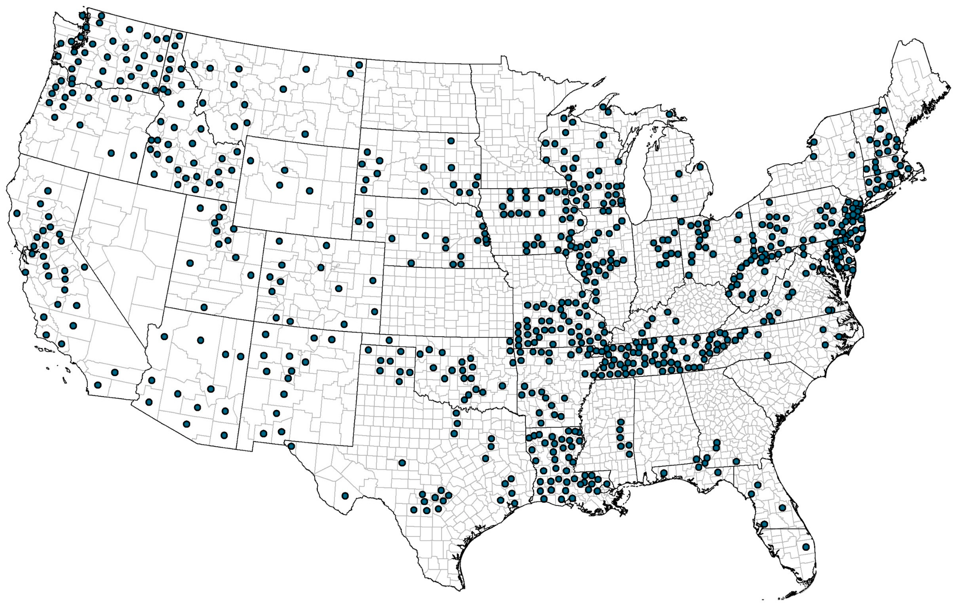
3.1. Location
3.2. Population Characteristics
3.2.1. Outcome
3.2.2. Exposure
3.2.3. Demographics
3.3. Poisson Regression Models
3.4. Sensitivity Analyses
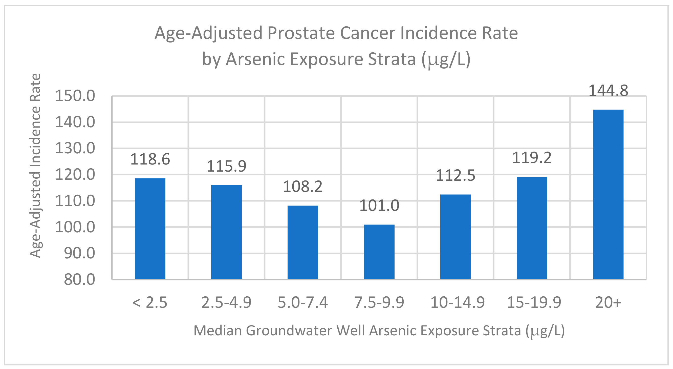
3.5. Stratified Analysis
4. Discussion
4.1. Epidemiological Studies
4.2. Arsenic metabolism
4.3. Arsenic Toxicology
4.4. Carcinogenicity Studies
4.5. Mode of Action
4.6. Dose-Response Models
4.7. Strengths and Limitations
5. Conclusions
Author Contributions
Funding
Acknowledgments
Conflicts of Interest
References
- United States Environmental Protection Agency (US EPA). National Primary Drinking Water Regulations; Arsenic and Clarifications to Compliance and New Source Contaminants Monitoring: Final rule; Federal Register, 40 CFR parts 9, 141, and 142; United States Environmental Protection Agency: Washington, DC, USA, 2001; pp. 6976–7066.
- Chen, C.J.; Kuo, T.L.; Wu, M.M. Arsenic and cancers. Lancet 1988, 1, 414–415. [Google Scholar] [CrossRef]
- Wu, M.M.; Kuo, T.L.; Hwang, Y.H.; Chen, C.J. Dose-response relationship between arsenic concentrations in well water and mortality from cancers and vascular diseases. Am. J. Epidemiol. 1989, 130, 1123–1132. [Google Scholar] [CrossRef] [PubMed]
- Chen, C.J.; Wang, C.J. Ecological correlation between arsenic level in well water and age-adjusted mortality from malignant neoplasms. Cancer Res. 1990, 50, 5470–5474. [Google Scholar] [PubMed]
- Tsai, S.M.; Wang, T.N.; Ko, Y.C. Mortality for certain diseases in areas with high levels of arsenic in drinking water. Arch. Environ. Health 1999, 54, 180–193. [Google Scholar] [CrossRef] [PubMed]
- Hinwood, A.L.; Jolley, D.J.; Sim, M.R. Cancer incidence and high environmental arsenic concentrations in rural populations: Results of an ecological study. Int. J. Environ. Health Res. 1999, 9, 131–141. [Google Scholar] [CrossRef]
- Lewis, D.R.; Southwick, J.W.; Ouellet-Hellstrom, R.; Rench, J.; Calderon, R.L. Drinking water arsenic in Utah: A cohort mortality study. Environ. Health Perspect. 1999, 107, 359–365. [Google Scholar] [CrossRef]
- Baastrup, R.; Sørensen, M.; Balstrøm, T.; Frederiksen, K.; Larsen, C.L.; Tjønneland, A.; Overvad, K.; Raaschou-Nielsen, O. Arsenic in drinking-water and risk for cancer in Denmark. Environ. Health Perspect. 2008, 116, 231–237. [Google Scholar] [CrossRef]
- García-Esquinas, E.; Pollan, M.; Umans, J.G.; Francesconi, K.A.; Goessler, W.; Guallar, E.; Howard, B.; Farley, J.; Best, L.G.; Navas-Acien, A. Arsenic exposure and cancer mortality in a US-based prospective cohort: The Strong Heart Study. Cancer Epidemiol. Biomarkers Prev. 2013, 22, 1944–1953. [Google Scholar]
- Bulka, C.M.; Jones, R.M.; Turyk, M.E.; Stayner, L.T.; Argos, M. Arsenic in drinking water and prostate cancer in Illinois counties: An ecologic study. Environ. Res. 2016, 148, 450–456. [Google Scholar] [CrossRef] [Green Version]
- Roh, T.; Lynch, C.F.; Weyer, P.; Wang, K.; Kelly, K.M.; Ludewig, G. Low-level arsenic exposure from drinking water is associated with prostate cancer in Iowa. Environ. Res. 2017, 159, 338–343. [Google Scholar] [CrossRef]
- Lamm, S.H.; Boroje, I.J.; Ferdosi, H.; Ahn, J. Lung cancer risk and low (≤50 μg/L) drinking water arsenic levels for US counties (2009–2013) - a negative association. Int. J. Environ. Res. Public Health 2018, 15, 1200. [Google Scholar] [CrossRef] [PubMed] [Green Version]
- United States Geological Survey (USGS). Metals and Other Trace Elements. Available online: http://water.usgs.gov/nawqa/trace/data/arsenic_nov2001 (accessed on 11 February 2013).
- Nadler, D.L.; Zudbenko, I.G. Estimating Cancer Latency Times Using a Weibull Model. Adv. Epidemiol. 2014, 2014. [Google Scholar] [CrossRef]
- United States Geological Survey (USGS). Available online: http://www.USGS/WaterUse/Data (accessed on 15 December 2016).
- Mendez, W.M., Jr.; Eftim, S.; Cohen, J.; Warren, I.; Crowden, J.; Lee, J.S.; Sams, R. Relationships between arsenic concentrations in drinking water and lung and bladder cancer incidence in U.S. counties. J. Expo. Sci. Environ. Epidemiol. 2017, 27, 235–243. [Google Scholar] [CrossRef] [PubMed]
- National Cancer Institute (NCI). Model-Based Small Area Estimates of Cancer Risk Factors and Screening Behaviors. 2016. Available online: http://sae.cancer.gov/nhis-brfss/methodology.html (accessed on 11 October 2016).
- United states Environmental Protection Agency (US EPA). Available online: https://www.epa.gov/radon/epa-map-radon-zones (accessed on 6 March 2018).
- National Cancer Institute (NCI). Available online: https://www.statecancerprofiles.cancer.gov/incidencerates/ (accessed on 26 September 2017).
- United States Census Bureau. American Fact Finder. Available online: https://factfinder.census.gov (accessed on 7 August 2017).
- Centers for Disease Control and Prevention (CDC). Diabetes Data and Trends. 2016. Available online: https://www.cdc.gov/diabetes/data/countydata/countydataindicators.htmlb (accessed on 27 March 2018).
- Lamm, S.H.; Ferdosi, H.; Dissen, E.K.; Ahn, J. A systematic review and meta-regression analysis of lung cancer risk and inorganic arsenic in drinking water. Int. J. Environ. Res. Public Health 2015, 12, 15498–15515. [Google Scholar] [CrossRef] [PubMed] [Green Version]
- Cook, R.D.; Weisberg, S. Residuals and Influence in Regression; Chapman & Hall: New York, NY, USA, 1982. [Google Scholar]
- Drobna, Z.; Styblo, M.; Thomas, D.J. An overview of arsenic metabolism and toxicity. Curr. Protoc. Toxicol. 2009, 42, 4–31. [Google Scholar] [PubMed] [Green Version]
- Abernathy, C.O.; Liu, Y.P.; Longfellow, D.; Aposhian, H.V.; Beck, B.; Fowler, B.; Goyer, R.; Menzer, R.; Rossman, T.; Thompson, C.; et al. Arsenic: Health effects, mechanisms of actions, and research issues. Environ. Health Perspect 1999, 107, 593–597. [Google Scholar] [CrossRef] [PubMed]
- Benbrahim-Tallaa, L.; Waalkes, M.P. Inorganic arsenic and human prostate cancer. Environ. Health Perspect. 2008, 116, 158–164. [Google Scholar] [CrossRef]
- Mann, S.; Droz, P.O.; Vahter, M. A physiologically based pharmacokinetic model for arsenic exposure. II. Validation and application in human. Toxicol. Appl. Pharmacol. 1996, 140, 471–486. [Google Scholar] [CrossRef]
- Styblo, M.; Del Razo, L.M.; Vega, L.; Germolec, D.R.; LeCluyse, E.L.; Hamilton, G.A.; Reed, W.; Wang, C.; Cullen, W.R.; Thomas, D.J. Comparative toxicity of trivalent and pentavalent inorganic and methylated arsenicals in rat and human cells. Arch. Toxicol. 2000, 74, 289–299. [Google Scholar] [CrossRef]
- Gentry, P.R.; McDonald, T.B.; Sullivan, D.E.; Shipp, A.M.; Yager, J.W.; Clewell, H.J. Analysis of genomic dose-response information on arsenic to inform key events in a mode of action for carcinogenicity. Environ. Mol. Mutagen. 2010, 51, 1–14. [Google Scholar] [CrossRef]
- Cohen, S.M.; Arnold, L.L.; Uzvolgyi, E.; Cano, M.; St John, M.; Yamamoto, S.; Lu, X.; Le, X.C. Possible role of dimethylarsinous acid in dimethylarsinic acid-induced urothelial toxicity and regeneration in the rat. Chem. Res. Toxicol. 2002, 15, 1150–1157. [Google Scholar] [CrossRef] [PubMed]
- Tsuji, J.S.; Chang, E.T.; Gentry, P.R.; Clewell, H.J.; Bofetta, P.; Cohen, S.M. Dose-response for assessing the cancer risk of inorganic arsenic in drinking water: The scientific basis for use of a threshold approach. Crit. Rev. Toxicol. 2019, 1, 1–49. [Google Scholar] [CrossRef] [PubMed]
- Snow, E.T.; Sykora, P.; Durham, T.R.; Klein, C.B. Arsenic, mode of action at biologically plausible low doses: What are the implications for low dose cancer risk? Toxicol. Appl. Pharmacol. 2005, 207, 557–564. [Google Scholar] [CrossRef] [PubMed]
- Yager, J.W.; Gentry, P.R.; Thomas, R.S.; Pluta, L.; Efremenko, A.; Black, M.; Arnold, L.L.; McKim, J.M.; Wilga, P.; Gill, G.; et al. Evaluation of gene expression changes in human primary uroepithelial cells following 24-hr exposures to inorganic arsenic and its methylated metabolites. Environ. Mol. Mutagen. 2013, 54, 82–98. [Google Scholar] [CrossRef] [PubMed]
- Shen, S.; Li, X.F.; Cullen, W.R.; Weinfeld, M.; Le, X.C. Arsenic binding to protein. Chem. Rev. 2013, 113, 7769–7792. [Google Scholar] [CrossRef]
- Waalkes, M.P.; Ward, J.M.; Liu, J.; Diwan, B.A. Transplacental carcinogenicity of inorganic arsenic in the drinking water: Induction of hepatic, ovarian, pulmonary, and adrenal tumors in mice. Toxicol. Appl. Pharmacol. 2003, 186, 7–17. [Google Scholar] [CrossRef]
- Waalkes, M.P.; Ward, J.M.; Diwan, B.A. Induction of tumors of the liver, lung, ovary, and adrenal in adult mice after brief maternal exposure to inorganic arsenic: Promotional effects from post-natal phorbol ester exposure on hepatic and pulmonary, but not dermal cancers. Carcinogenesis 2004, 25, 133–141. [Google Scholar] [CrossRef] [Green Version]
- Waalkes, M.P.; Liu, J.; Ward, J.M.; Powell, D.A.; Diwan, B.A. Urogenital carcinogenesis in female CD1 mice induced by in-utero arsenic exposure is exacerbated by post-natal diethylstilbesterol treatment. Cancer Res. 2006, 66, 1337–1345. [Google Scholar] [CrossRef] [Green Version]
- Waalkes, M.P.; Liu, J.; Ward, J.M.; Diwan, B.A. Enhanced urinary bladder and liver carcinogenesis in male CD1 mice exposed to transplacental inorganic arsenic and postnatal diethylstilbesterol or tamoxifen. Toxicol. Appl. Pharmacol. 2006, 215, 295–305. [Google Scholar] [CrossRef]
- Tokar, E.J.; Diwan, B.A.; Ward, J.M.; Delker, D.A.; Waalkes, M.P. Carcinogenic effects of whole-life exposure to inorganic arsenic in CD1 mice. Toxicol. Sci. 2011, 119, 73–83. [Google Scholar] [CrossRef]
- Waalkes, M.P.; Qu, W.; Tokar, E.J.; Kissling, G.E.; Dixon, D. Lung tumors in mice induced by whole-life inorganic arsenic exposure at human-relevant doses. Arch. Toxicol. 2014, 88, 1–11. [Google Scholar]
- Nesnow, S.; Roop, B.C.; Lambert, G.; Kadiiska, M.; Masan, R.P.; Cullen, W.R.; Mass, M.J. DNA damage induced by methylated trivalent arsenicals is mediated by reactive oxygen species. Chem. Res. Toxicol. 2002, 15, 1627–1634. [Google Scholar] [CrossRef] [PubMed]
- Cohen, S.M.; Arnold, L.L.; Beck, B.D.; Lewis, A.S.; Eldan, M. Evaluation of the carcinogenicity of inorganic arsenic. Crit. Rev. Toxicol. 2013, 43, 711–752. [Google Scholar] [CrossRef] [PubMed]
- Cohen, S.M.; Arnold, L.L.; Eldan, M.; Lewis, A.S.; Beck, B.D. Methylated arsenicals: The implications of metabolism and carcinogenicity studies in rodents to human risk assessment. Crit. Rev. Toxicol. 2006, 36, 99–133. [Google Scholar] [CrossRef]
- Cohen, S.M.; Purtilo, D.T.; Ellwein, L.B. Ideas in pathology. Pivotal role of increased cell proliferation in human carcinogenesis. Mod. Pathol. 1991, 4, 371–382. [Google Scholar]
- Dodson, M.; de la Vega, M.R.; Harder, B.; Castro-Portuguez, R.; Rodrigues, S.D.; Wong, P.K.; Chapman, E.; Zhang, D.D. Low-level arsenic causes proteotoxic stress and not oxidative stress. Toxicol. Appl. Pharmacol. 2018, 341, 106–113. [Google Scholar] [CrossRef]
- Lau, A.; Whitman, S.A.; Jaramillo, M.C.; Zhang, D.D. Arsenic-mediated activation of the Nrf2-Keap1 antioxidant pathway. J. Biochem. Mol. Toxicol. 2013, 27, 99–105. [Google Scholar] [CrossRef]
- Clewell, H.J.; Thomas, R.S.; Kenyon, E.M.; Hughes, M.F.; Adair, B.M.; Gentry, P.R.; Yager, J.W. Concentration- and time-dependent genomic changes in the mouse urinary bladder following exposure to arsenate in drinking water for up to 12 weeks. Toxicol. Sci. 2011, 123, 421–432. [Google Scholar] [CrossRef] [Green Version]
- Achanzar, W.E.; Brambila, E.M.; Diwan, B.A.; Webber, M.M.; Waalkes, M.P. Inorganic arsenite-induced malignant transformation of human prostate epithelial cells. J. Natl. Cancer Inst. 2002, 94, 1888–1891. [Google Scholar] [CrossRef] [Green Version]
- Kojima, C.; Ramirez, D.C.; Tokar, E.J.; Himeno, S.; Drobna, Z.; Styblo, M.; Mason, R.P.; Waakles, M.P. Requirement of arsenic biomethylation for oxidative DNA damage. J. Natl. Cancer Inst. 2009, 101, 1670–1681. [Google Scholar] [CrossRef] [Green Version]
- Lamm, S.H.; Luo, Z.D.; Bo, F.B.; Zhang, G.Y.; Zhang, Y.M.; Wilson, R.; Byrd, D.M.; Lai, S.; Li, F.X.; Polkanov, M.; et al. An epidemiological study of arsenic-related skin disorders and skin cancer and the consumption of arsenic-contaminated well waters in Huhhot, Inner Mongolia, China. Hum. Ecol. Risk Anal. 2007, 13, 713–746. [Google Scholar] [CrossRef]
- Lamm, S.H.; Engel, A.; Penn, C.; Chen, R.; Feinleib, M. Letter to Scientific Advisory Board Arsenic Review Panel; USEPA Science Advisory Board: Washington, DC, USA, 19 August 2005.

| Variable | Median | Mean | Minimum | Maximum |
|---|---|---|---|---|
| Outcome | ||||
| Prostate Cancer Rate (per 100,000) | 116.4 | 117.9 | 44.8 | 220.3 |
| Count (5-year estimate) | 111 | 442 | 10 | 12,652 |
| Exposure | ||||
| Dependency | 87% | 76% | 10% | 100% |
| Well Count | 2 | 8.1 | 1 | 190 |
| As Median (ug/L) | 0.9 | 2.1 | 0.7 | 52.5 |
| As Minimum (μg/L) | 0.7 | 1.3 | 0.7 | 42 |
| As Maximum (μg/L) | 1.0 | 7.96 | 0.7 | 190 |
| Co-Variates | ||||
| Current Smoker (%) | 25.6 | 25.3 | 9.54 | 40.0 |
| Ex-Smoker (%) | 29.6 | 29.9 | 15.9 | 48.3 |
| Obesity (%) | 31.9 | 31.2 | 15.1 | 41.2 |
| Education (<HS) (%) | 84.3 | 83.0 | 58.6 | 97.4 |
| Residency (Same County) (%) | 94 | 93 | 78 | 98 |
| Poverty (%) | 14 | 15 | 3 | 48 |
| Income ($K) | 44.8 | 47.3 | 23.9 | 106.1 |
| Rural (%) | 48 | 49 | 0 | 100 |
| Population | ||||
| Male Population | 19,977 | 71,914 | 1,698 | 2,037,405 |
| Hispanic (%) | 4 | 9 | 0 | 80 |
| White (%) | 92 | 87 | 20 | 99 |
| Black (%) | 2 | 7 | 0 | 69 |
| Asian (%) | 1 | 1 | 0 | 22 |
| Other (%) | 2 | 4 | 1 | 79 |
| Unadjusted | Exposure Range for Median Arsenic Level | ||
|---|---|---|---|
| All | Without Outliers | Without Non-Significants + | |
| Unadjusted Median Model | |||
| N | 715 | 712 | 712 |
| Arsenic2 | 0.0007 *** | 0.0005 *** | 0.0005 *** |
| Arsenic | −0.0310 *** | −0.0225 *** | −0.0225 *** |
| Intercept | −5.0460 *** | −5.0480 *** | −5.0480 *** |
| Adjusted | All | Without Outliers | Without Non-Significants + |
| Adjusted Median Model | |||
| N | 710 | 707 | 707 |
| Arsenic2 | 0.0003 *** | 0.0002 *** | 0.0002 *** |
| Arsenic | −0.0105 *** | −0.0044 ** | −0.0043 ** |
| GW Dependency | 0.0243 *** | 0.0204 ** | 0.0196 ** |
| Current Smoker | −0.0031 *** | −0.0019 ** | −0.0192 ** |
| Ex-Smoker | 0.0016 * | 0.0002 | - |
| Radon (>4 pCi/L) | −0.0229 *** | −0.0380 *** | −0.02869 *** |
| Obesity | −0.0044 *** | −0.0028 *** | −0.0029 *** |
| Education (<HS grad) | −0.0023 *** | −0.0001 | - |
| Residency (Same cnty) | 0.5992 *** | 0.9458 *** | 0.9353 *** |
| Income (MHHI $K) | 0.0001 | 0.0006 | −0.8308 *** |
| Poverty | −0.9332 *** | −0.8308 *** | - |
| Rural | −0.0976 *** | −0.0972 *** | −0.0952 *** |
| Hispanic | −0.2762 *** | 0.7371 *** | 0.2969 *** |
| Black | 0.7872 *** | −0.2438 *** | −0.7414 *** |
| Asian | 0.1804 *** | 0.370 | - |
| Other | −0.1993 *** | −0.1950 *** | −0.1988 *** |
| Intercept | −5.1643 *** | −5.7424 *** | −5.7519 *** |
| Variable | Maximum + <100 μg/L | Median + <50 μg/L | Dependency > 80 μg/L |
|---|---|---|---|
| N | 695 | 707 | 392 |
| Arsenic2 | 0.0001 ** | 0.0002 *** | 0.0003 *** |
| Arsenic | −0.0015 | −0.0044 ** | −0.0090 *** |
| GW Dependency | 0.0354 *** | 0.0204 ** | −0.3562 *** |
| Current Smoker | −0.0010 | −0.0019 ** | −0.0026 ** |
| Ex-Smoker | −0.0010 | −0.0002 | −0.00465 *** |
| Radon (>4 pCi/L) | −0.0397 *** | −0.0380 *** | −0.0491 *** |
| Obesity | −0.0040 | −0.0028 *** | −0.0046 *** |
| Education (<HS grad) | 0.0029 *** | −0.0001 | 0.0038 *** |
| Residency (same cnty) | 1.1929 *** | 0.9458 *** | 1.4419 *** |
| Income (MHHI $K) | −0.0004 | 0.0006 | 0.0017 ** |
| Poverty | −0.7191 *** | −0.8193 *** | −0.6423 *** |
| Rural | −0.0813 *** | −0.0972 *** | −0.0966 *** |
| Hispanic | −0.1367 *** | 0.2371 *** | −0.4040 *** |
| Black | 0.7731 *** | 0.7438 *** | 0.5714 *** |
| Asian | −0.0387 | −0.0370 | 0.5339 *** |
| Other | −0.2432 *** | −0.1950 ** | −0.4291 *** |
| Intercept | −6.2642 *** | −5.7423 *** | −5.6349 *** |
| Regression Model | Poisson | Negative-Binomial |
|---|---|---|
| Adjusted Median Model | ||
| N | 710 | 710 |
| Arsenic2 | 0.0003 *** | 0.0002 * |
| Arsenic | −0.0105 *** | −0.0050 |
| GW Dependency | 0.0243 *** | 0.0432 |
| Current Smoker | −0.0031 *** | −0.0068 ** |
| Ex-Smoker | 0.0016 * | −0.0014 |
| Radon (>4 pCi/L) | −0.0229 *** | 0.0086 |
| Obesity | −0.0044 *** | −0.0003 |
| Education (<HS grad) | −0.0023 *** | 0.0011 |
| Residency (same cnty) | 0.5992 *** | 0.7427 ** |
| Income (MHHI $K) | 0.0001 | −0.0005 |
| Poverty | −0.9332 *** | −0.7564 ** |
| Rural | −0.0976 *** | −0.1123 ** |
| Hispanic | -0.0262 *** | −0.2405 * |
| Black | 0.7872 *** | 0.7987 *** |
| Asian | 0.1804 *** | −0.0654 |
| Other | −0.1993 *** | −0.1028 |
| Intercept | −5.1643 *** | −5.5708 *** |
© 2020 by the authors. Licensee MDPI, Basel, Switzerland. This article is an open access article distributed under the terms and conditions of the Creative Commons Attribution (CC BY) license (http://creativecommons.org/licenses/by/4.0/).
Share and Cite
Ahn, J.; Boroje, I.J.; Ferdosi, H.; Kramer, Z.J.; Lamm, S.H. Prostate Cancer Incidence in U.S. Counties and Low Levels of Arsenic in Drinking Water. Int. J. Environ. Res. Public Health 2020, 17, 960. https://doi.org/10.3390/ijerph17030960
Ahn J, Boroje IJ, Ferdosi H, Kramer ZJ, Lamm SH. Prostate Cancer Incidence in U.S. Counties and Low Levels of Arsenic in Drinking Water. International Journal of Environmental Research and Public Health. 2020; 17(3):960. https://doi.org/10.3390/ijerph17030960
Chicago/Turabian StyleAhn, Jaeil, Isabella J. Boroje, Hamid Ferdosi, Zachary J. Kramer, and Steven H. Lamm. 2020. "Prostate Cancer Incidence in U.S. Counties and Low Levels of Arsenic in Drinking Water" International Journal of Environmental Research and Public Health 17, no. 3: 960. https://doi.org/10.3390/ijerph17030960