
Testing the Energy-Environmental Kuznets Curve Hypothesis in the Renewable and Nonrenewable Energy Consumption Models in Egypt


Abstract
:1. Introduction
2. Literature Review
3. Methods
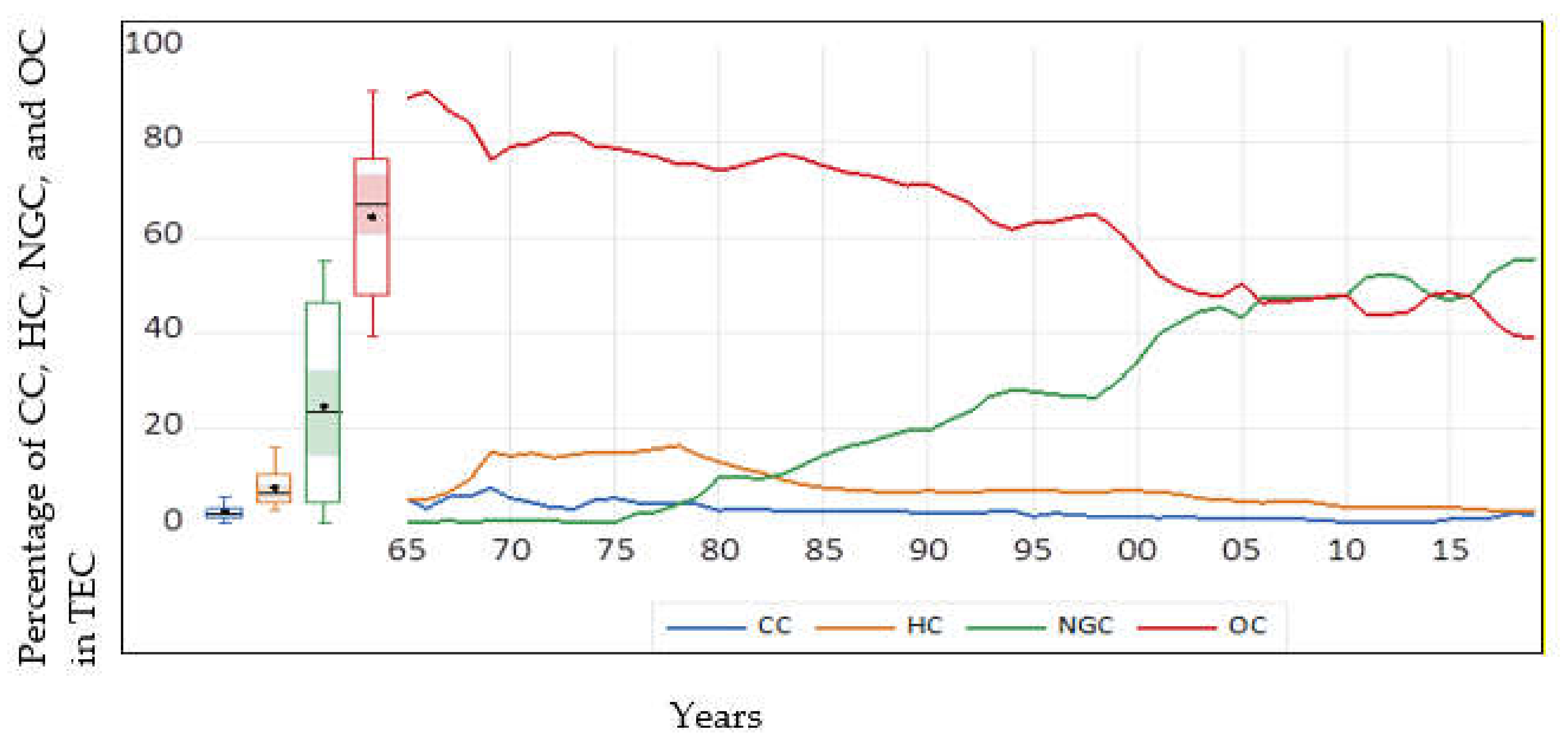
4. Results
5. Conclusions
Author Contributions
Funding
Institutional Review Board Statement
Informed Consent Statement
Data Availability Statement
Acknowledgments
Conflicts of Interest
References
- Grossman, G.M.; Krueger, A.B. Environmental Impacts of the North American Free Trade Agreement. NBER, Working Paper 3914. 1991. Available online: https://www.nber.org/papers/w3914 (accessed on 15 March 2021).
- Panayotou, T. Empirical Tests and Policy Analysis of Environmental Degradation at Different Stages of Economic Development; ILO, Technology and Employment Programme: Geneva, Switzerland, 1993. [Google Scholar]
- Kuznets, S. Economic growth and income inequality. Am. Econ. Rev. 1955, 45, 1–28. [Google Scholar]
- Mahmood, H.; Maalel, N.; Hassan, M.S. Probing the Energy-Environmental Kuznets Curve Hypothesis in the Oil and Natural Gas Consumption models Considering Urbanization and Financial Development in the Middle East Countries. Energies 2021, 14, 3178. [Google Scholar] [CrossRef]
- Simionescu, M.; Păuna, C.B.; Niculescu, M.-D.V. The Relationship between Economic Growth and Pollution in Some New European Union Member States: A Dynamic Panel ARDL Approach. Energies 2021, 14, 2363. [Google Scholar] [CrossRef]
- Alola, A.A.; Donve, U.T. Environmental Implication of Coal and Oil Energy Utilization in Turkey: Is the EKC Hypothesis related to Energy? Manag. Environ. Qual. 2021, 32, 543–559. [Google Scholar] [CrossRef]
- Chang, D.S.; Yeh, L.T.; Chen, Y. The Effects of Economic Development, International Trade, Industrial Structure and Energy Demands on Sustainable Development. Sustain. Dev. 2014, 22, 377–390. [Google Scholar] [CrossRef]
- Zarzoso, I.M.; Motrancho, A.B. Pooled Mean Group Estimation of an Environmental Kuznets Curve for CO2. Econ. Lett. 2004, 82, 121–126. [Google Scholar] [CrossRef]
- Mahmood, H.; Alrasheed, A.S.; Furqan, M. Financial Market Development and Pollution Nexus in Saudi Arabia: Asymmetrical Analysis. Energies 2018, 11, 3462. [Google Scholar] [CrossRef] [Green Version]
- Suri, V.; Chapman, D. Economic Growth, Trade and Energy: Implications for the Environmental Kuznets Curve. Ecol. Econ. 1998, 25, 195–208. [Google Scholar] [CrossRef]
- Aruga, K. Investigating the Energy-Environmental Kuznets Curve Hypothesis for the Asia-Pacific Region. Sustainability 2019, 11, 2395. [Google Scholar] [CrossRef] [Green Version]
- Hundie, S.K.; Daksa, M.D. Does Energy-Environmental Kuznets Curve Hold for Ethiopia? The Relationship between Energy Intensity and Economic Growth. J. Econ. Struct. 2019, 8, 21. [Google Scholar] [CrossRef]
- Aboagye, S. The Policy Implications of the Relationship between Energy Consumption, Energy Intensity and Economic Growth in Ghana. OPEC Energy Rev. 2017, 41, 344–363. [Google Scholar] [CrossRef]
- Luzzati, T.; Orsini, M. Investigating the Energy-Environmental Kuznets Curve. Energy 2009, 34, 291–300. [Google Scholar] [CrossRef]
- Pablo-Romero, M.D.P.; De Jesus, J. Economic Growth and Energy Consumption: The Energy-Environmental Kuznets Curve for Latin America and the Caribbean. Renew. Sustain. Energy Rev. 2016, 60, 1343–1350. [Google Scholar] [CrossRef]
- BP. BP Statistical Review of World Energy. 2021. Available online: https://www.bp.com/statisticalreview (accessed on 21 March 2021).
- National Energy Technology Laboratory. Cost and Performance Baseline for Fossil Energy Plants; United States Department of Energy No. DOE/NETL-2010/1397; National Energy Technology Laboratory: Morgantown, WV, USA, 2010. [Google Scholar]
- Park, S. American Security Project (ASP)’s Report on Energy in Egypt: Background and Issues. 2015. Available online: https://www.americansecurityproject.org/wp-content/uploads/2015/03/Ref-0190-Energy-in-Egypt-Background-and-Issues.pdf (accessed on 15 April 2021).
- Abdel-Khalek, G. Income and price elasticities of energy consumption in Egypt: A time-series analysis. Energy Econ. 1988, 10, 47–58. [Google Scholar] [CrossRef]
- Sharaf, M.F. Energy consumption and economic growth: A disaggregated causality analysis with structural breaks. Reg. Dev. 2017, 46, 59–76. [Google Scholar]
- Li, S.; Shi, J.; Wu, Q. Environmental Kuznets Curve: Empirical Relationship between Energy Consumption and Economic Growth in Upper-Middle-Income Regions of China. Int. J. Environ. Res. Public Health 2020, 17, 6971. [Google Scholar] [CrossRef] [PubMed]
- Ge, X.; Zhou, Z.; Zhou, Y.; Ye, X.; Liu, S. A Spatial Panel Data Analysis of Economic Growth, Urbanization, and NOx Emissions in China. Int. J. Environ. Res. Public Health 2018, 15, 725. [Google Scholar] [CrossRef] [Green Version]
- Ibrahiem, D.M. Renewable electricity consumption, foreign direct investment and economic growth in Egypt: An ARDL approach. Procedia Econ. Financ. 2015, 30, 313–323. [Google Scholar] [CrossRef] [Green Version]
- Kwakwa, P.A. Electricity consumption in Egypt: A long-run analysis of its determinants. OPEC Energy Rev. 2017, 41, 3–22. [Google Scholar] [CrossRef]
- Ibrahiem, D.M. Environmental Kuznets curve: An empirical analysis for carbon dioxide emissions in Egypt. Int. J. Green Econ. 2016, 10, 136–150. [Google Scholar] [CrossRef]
- Mahmood, H.; Furqan, M.; Alkhateeb, T.T.Y.; Fawaz, M.M. Testing the environmental Kuznets curve in Egypt: Role of foreign investment and trade. Int. J. Energy Econ. Policy 2019, 9, 225–228. [Google Scholar]
- El-Aasar, K.M.; Hanafy, S.A. Investigating the environmental Kuznets curve hypothesis in Egypt: The role of renewable energy and trade in mitigating GHGs. Int. J. Energy Econ. Policy 2018, 8, 177–184. [Google Scholar]
- Beşe, E.; Kalayci, S. Testing the environmental Kuznets curve hypothesis: Evidence from Egypt, Kenya and Turkey. Int. J. Energy Econ. Policy 2019, 9, 479–491. [Google Scholar] [CrossRef]
- Moosa, I.A. Growth and environmental degradation in MENA countries: Methodological issues and empirical evidence. Middle East Dev. J. 2019, 11, 251–269. [Google Scholar] [CrossRef]
- Sghaier, A.; Guizani, A.; Ben Jabeur, S.; Nurunnabi, M. Tourism development, energy consumption and environmental quality in Tunisia, Egypt and Morocco: A trivariate analysis. GeoJournal 2019, 84, 593–609. [Google Scholar] [CrossRef]
- Fethi, S.; Senyucel, E. The role of tourism development on CO2 emission reduction in an extended version of the environmental Kuznets curve: Evidence from top 50 tourist destination countries. Environ. Dev. Sustain. 2021, 23, 1499–1524. [Google Scholar] [CrossRef]
- Copeland, B.R.; Taylor, M.S. Trade and environment: A partial synthesis. Am. J. Agric. Econ. 1995, 77, 765–771. [Google Scholar] [CrossRef]
- Hettige, H.; Lucas, R.E.B.; Wheeler, D. The toxic intensity of industrial production: Global patterns, trends, and trade policy. Am. Econ. Rev. 1992, 82, 478–481. [Google Scholar]
- Saint-Paul, G. Chapter 2. In The Economics of Sustainable Development; Goldin, I., Winter, A.L., Eds.; Cambridge University Press: Cambridge, UK, 1994; pp. 47–50. [Google Scholar]
- Rock, M.T. Pollution intensity of GDP and trade policy: Can the World Bank be wrong. World Dev. 1996, 24, 471–479. [Google Scholar] [CrossRef]
- Grossman, G.M.; Krueger, A.B. Economic growth and the environment. Q. J. Econ. 1995, 110, 353–377. [Google Scholar] [CrossRef] [Green Version]
- Antweiler, W.; Copeland, B.R.; Taylor, M.S. Is free trade good for the environment? Am. Econ. Rev. 2001, 91, 877–908. [Google Scholar] [CrossRef] [Green Version]
- Arrow, K.; Bolin, B.; Costanza, R.; Folke, C.; Holling, C.S.; Janson, B.; Levin, S.; Maler, K.; Perrings, C.; Pimental, D. Economic growth, carrying capacity, and the environment. Science 1995, 15, 91–95. [Google Scholar]
- Coondoo, D.; Dinda, S. Causality between income and emission: A country group-specific econometric analysis. Ecol. Econ. 2002, 40, 351–367. [Google Scholar] [CrossRef]
- Lucas, R.E.B.; Wheeler, D.; Hettige, H. Economic Development, Environmental Regulation and the International Migration of Toxic Industrial Pollution: 1960–1988; International Trade and the Environment. World Bank Discussion Paper No. 159; World Bank: Washington, DC, USA, 1992. [Google Scholar]
- Stern, D.I. The Rise and Fall of the Environmental Kuznets Curve. World Dev. 2004, 32, 1419–1439. [Google Scholar] [CrossRef]
- Stern, D.I.; Common, M.S. Is there an environmental Kuznets curve for sulfur? J. Environ. Econ. Manag. 2001, 41, 162–217. [Google Scholar] [CrossRef] [Green Version]
- Millimet, D.L.; List, J.A.; Stengos, T. The environmental Kuznets curve: Real progress or misspecified models? Rev. Econ. Stat. 2003, 85, 1038–1047. [Google Scholar] [CrossRef]
- Akkemike, K.A.; Göksal, K. Energy Consumption-GDP Nexus: Heterogeneous panel causality analysis. Energy Econ. 2012, 34, 865–873. [Google Scholar] [CrossRef]
- Payne, J.E. On the dynamics of energy consumption and output in the US. Appl. Energy 2009, 86, 575–577. [Google Scholar] [CrossRef]
- Ouedraogo, N.S. Energy consumption and economic growth: Evidence from the economic community of West African states (ECOWAS). Energy Econ. 2013, 36, 637–647. [Google Scholar] [CrossRef]
- Huang, B.; Hwang, M.; Yang, C.W. 2008. Causal relationship between energy consumption and GDP growth revisited: A dynamic panel data approach. Ecol. Econ. 2008, 67, 41–54. [Google Scholar] [CrossRef]
- Shahbaz, M.; Lean, H.H.; Shabbir, M.S. Environmental Kuznets Curve Hypothesis in Pakistan: Cointegration and Granger Causality. Renew. Sustain. Energy Rev. 2012, 16, 2947–2953. [Google Scholar] [CrossRef] [Green Version]
- Nasir, M.; Rehman, F.U. Environmental Kuznets Curve for Carbon Emissions in Pakistan: An Empirical Investigation. Energy Policy 2011, 39, 1857–1864. [Google Scholar] [CrossRef]
- Shahbaz, M.; Mallick, H.; Mahalik, M.K.; Loganathan, N. Does globalization Impede Environmental Quality in India? Ecol. Indic. 2015, 52, 379–393. [Google Scholar] [CrossRef] [Green Version]
- Bayer, C.; Hanck, C. Combining Non-Cointegration Tests. J. Time Ser. Anal. 2013, 34, 83–95. [Google Scholar] [CrossRef]
- Jalil, A.; Mahmud, S.F. Environment Kuznets Curve for CO2 Emissions: A Cointegration Analysis for China. Energy Policy 2009, 37, 5167–5172. [Google Scholar] [CrossRef] [Green Version]
- Shahbaz, M.; Haouas, I.; Sohag, K.; Ozturk, I. The Financial Development-Environmental Degradation Nexus in the United Arab Emirates: The Importance of Growth, Globalization and Structural Breaks. Environ. Sci. Pollut. Res. 2020, 27, 10685–10699. [Google Scholar] [CrossRef] [Green Version]
- Ozturk, I.; Acaravci, A. The Long-Run and Causal Analysis of Energy, growth, Openness and Financial Development on Carbon Emissions in Turkey. Energy Econ. 2013, 36, 262–267. [Google Scholar] [CrossRef]
- Shahbaz, M.; Ozturk, I.; Afza, T.; Ali, A. Revisiting the Environmental Kuznets Curve in a Global Economy. Renew. Sustain. Energy Rev. 2013, 25, 494–502. [Google Scholar] [CrossRef] [Green Version]
- Ozatac, N.; Gokmenoglu, K.K.; Taspinar, N. Testing the EKC Hypothesis by Considering Trade Openness, Urbanization, and Financial Development: The Case of Turkey. Environ. Sci. Pollut. Res. 2017, 24, 16690–16701. [Google Scholar] [CrossRef]
- Acaravci, A.; Ozturk, I. On the Relationship between Energy Consumption, CO2 Emissions and Economic Growth in Europe. Energy 2010, 35, 5412–5420. [Google Scholar] [CrossRef]
- Madaleno, M.; Moutinho, V. Analysis of the New Kuznets Relationship: Considering Emissions of Carbon, Methanol, and Nitrous Oxide Greenhouse Gases—Evidence from EU Countries. Int. J. Environ. Res. Public Health 2021, 18, 2907. [Google Scholar] [CrossRef] [PubMed]
- To, A.H.; Ha, D.T.-T.; Nguyen, H.M.; Vo, D.H. The Impact of Foreign Direct Investment on Environment Degradation: Evidence from Emerging Markets in Asia. Int. J. Environ. Res. Public Health 2019, 16, 1636. [Google Scholar] [CrossRef] [Green Version]
- Javid, M.; Sharif, F. Environmental Kuznets Curve and Financial Development in Pakistan. Renew. Sustain. Energy Rev. 2016, 54, 406–414. [Google Scholar] [CrossRef]
- Murshed, M.; Alam, R.; Ansarin, A. The Environmental Kuznets Curve Hypothesis for Bangladesh: The Importance of Natural Gas, Liquefied Petroleum Gas, and Hydropower Consumption. Environ. Sci. Pollut. Res. 2021, 28, 17208–17227. [Google Scholar] [CrossRef]
- Rabbi, F.; Akbar, D.; Kabir, S.M.Z. Environment Kuznets Curve for Carbon Emissions: A Cointegration Analysis for Bangladesh. Int. J. Energy Econ. Policy 2015, 5, 45–53. [Google Scholar]
- Dong, K.; Sun, R.; Jiang, H.; Zeng, X. CO2 Emissions, Economic Growth, and the Environmental Kuznets Curve in China: What Roles Can Nuclear Energy and Renewable Energy Play? J. Clean. Prod. 2018, 196, 51–63. [Google Scholar] [CrossRef]
- Ren, S.; Yuan, B.; Ma, X.; Chen, X. International Trade, FDI (Foreign Direct Investment) and Embodied CO2 Emissions: A Case Study of Chinas Industrial Sectors. China Econ. Rev. 2014, 28, 123–134. [Google Scholar] [CrossRef]
- Farhani, S.; Lorente, D.B. Comparing the Role of Coal to other Energy Resources in the Environmental Kuznets Curve of three Large Economies. Chin. Econ. 2020, 53, 82–120. [Google Scholar] [CrossRef]
- Saboori, B.; Sulaiman, J.; Mohd, S. Environmental Kuznets Curve and Energy Consumption in Malaysia: A Cointegration Approach. Energy Sources Part B Econ. Plan. Policy 2016, 11, 861–867. [Google Scholar] [CrossRef]
- Saboori, B.; Sulaiman, J. Environmental Degradation, Economic Growth and Energy Consumption: Evidence of the Environmental Kuznets Curve in Malaysia. Energy Policy 2016, 60, 892–905. [Google Scholar] [CrossRef]
- Marques, A.C.; Fuinhas, J.A.; Leal, P.A. The Impact of Economic Growth on CO2 Emissions in Australia: The Environmental Kuznets Curve and the Decoupling Index. Environ. Sci. Pollut. Res. 2018, 25, 27283–27296. [Google Scholar] [CrossRef]
- Pata, U.K. The Influence of Coal and Noncarbohydrate Energy Consumption on CO2 Emissions: Revisiting the Environmental Kuznets Curve Hypothesis for Turkey. Energy 2018, 160, 1115–1123. [Google Scholar] [CrossRef]
- Bilgili, F.; Kocak, E.; Bulut, U.; Kuloglu, A. The Impact of Urbanization on Energy Intensity: Panel Data Evidence Considering Cross-Sectional Dependence and Heterogeneity. Energy 2017, 133, 242–256. [Google Scholar] [CrossRef]
- Kander, A.; Warde, P.; Henriques, S.T.; Nielsen, H.; Kulionis, V.; Hagen, S. International Trade and Energy Intensity during European Industrialization, 1870–1935. Ecol. Econ. 2017, 139, 33–44. [Google Scholar] [CrossRef]
- Onafowora, O.A.; Owoye, O. Bounds testing approach to analysis of the environment Kuznets curve hypothesis. Energy Econ. 2014, 44, 47–62. [Google Scholar] [CrossRef]
- Ahmed, K.; Ozturk, I.; Ghumro, I.A.; Mukesh, P. Effect of trade on ecological quality: A case of D-8 countries. Environ. Sci. Pollut. Res. 2019, 26, 35935–35944. [Google Scholar] [CrossRef] [PubMed]
- Sulaiman, C.; Abdul-Rahim, A.S. Can clean biomass energy use lower CO2 emissions in African economies? Empirical evidence from dynamic long-run panel framework. Environ. Sci. Pollut. Res. 2020, 27, 37699–37708. [Google Scholar] [CrossRef]
- World Bank. World Development Indicators; World Bank: Washington, DC, USA, 2021. [Google Scholar]
- Ng, S.; Perron, P. Lag Length Selection and the Construction of Unit Root Tests with Good Size and Power. Econometrica 2001, 69, 1519–1554. [Google Scholar] [CrossRef] [Green Version]
- Pesaran, M.H.; Shin, Y.; Smith, R.J. Structural analysis of vector error correction models with exogenous I(1) variables. J. Econ. 2001, 97, 293–343. [Google Scholar] [CrossRef] [Green Version]
- Kripfganz, S.; Schneider, D.C. Response Surface Regressions for Critical Value Bounds and Approximate p-Values in Equilibrium Correction Models; Economics Department Discussion Papers Series, Paper number 19/01; University of Exeter: Exeter, UK, 2019; Available online: http://people.exeter.ac.uk/RePEc/dpapers/DP1901.pdf (accessed on 18 March 2021).
- Diao, X.; Zeng, S.; Tam, C.; Tam, V. EKC analysis for studying economic growth and environmental quality: A case study in China. J. Clean Prod. 2019, 17, 541–548. [Google Scholar] [CrossRef]
- Gerundo, R.; Grimaldi, M.; Marra, A. A methodology hazard-based for the mitigation of the radon risk in the urban planning. UPLanD J. Urb. Plan. Landsc. Environ. Des. 2016, 1, 27–38. [Google Scholar]
- Gerundo, R.; Nesticò, A.; Marra, A.; Carotenuto, M. Peripheralization Risk Mitigation: A Decision Support Model to Evaluate Urban Regeneration Programs Effectiveness. Sustainability 2021, 12, 8024. [Google Scholar] [CrossRef]


| OCt | NGCt | CCt | PECt | HCt | GDPCt | |
|---|---|---|---|---|---|---|
| Mean | −0.224187 | −1.898542 | −3.575728 | 0.244363 | −2.411493 | 9.861380 |
| Median | −0.025270 | −1.078036 | −3.498677 | 0.364126 | −2.281486 | 9.908434 |
| Maximum | 0.567938 | 0.763329 | −2.406410 | 1.365439 | −1.941707 | 10.55649 |
| Minimum | −1.612627 | −6.378393 | −4.467861 | −1.341031 | −4.055660 | 9.082881 |
| Std. Dev. | 0.628077 | 2.467149 | 0.417401 | 0.843266 | 0.510672 | 0.470406 |
| Observations | 55 | 55 | 55 | 55 | 55 | 55 |
| Variable | Intercept | Intercept and Trend | ||||||
|---|---|---|---|---|---|---|---|---|
| PECt | −4.2658 | −1.2638 | 0.2963 | 6.0270 | −3.9478 | −1.2643 | 0.3203 | 21.4005 |
| OCt | 0.5895 | 0.6476 | 1.0985 | 75.7772 | −2.9230 | −1.0404 | 0.3560 | 26.7822 |
| NGCt | 0.8080 | 1.0480 | 1.2969 | 107.9720 | −2.3539 | −0.9181 | 0.3900 | 31.7657 |
| CCt | −2.6936 | −0.7081 | 0.2629 | 7.7003 | −8.3180 | −1.8994 | 0.2284 | 11.3901 |
| HCt | −0.8039 | −0.4699 | 0.5846 | 19.8411 | −5.0146 | −1.4586 | 0.2909 | 17.5758 |
| GDPCt | 0.9867 | 0.8374 | 0.8486 | 51.9301 | −9.0978 | −2.0891 | 0.2296 | 10.1875 |
| GDPCt2 | 1.0413 | 0.8770 | 0.8422 | 51.7753 | −15.0243 * | −2.7179 * | 0.1809 * | 6.2016 * |
| GDPCt3 | 1.0959 | 0.9141 | 0.8341 | 51.4475 | −18.1113 ** | −2.9987 ** | 0.1656 ** | 5.0958 ** |
| ΔPECt | −26.0071 *** | −3.5823 *** | 0.1377 *** | 1.0198 *** | −25.9332 *** | −3.5905 *** | 0.1385 *** | 3.5789 *** |
| ΔOCt | −26.4147 *** | −3.6155 *** | 0.1369 *** | 0.9885 *** | −26.2858 *** | −3.6236 *** | 0.1379 *** | 3.4769 *** |
| ΔNGCt | −35.7491 *** | −4.2218 *** | 0.1181 *** | 0.7030 *** | −140.6270 *** | −8.3848 *** | 0.0596 *** | 0.6496 *** |
| ΔCCt | −4.3428 | −1.4666 | 0.3376 | 5.6538 | −25.7829 *** | −3.5668 *** | 0.1383 *** | 3.6748 *** |
| ΔHCt | −16.7487 *** | −2.8835 *** | 0.1722 *** | 1.5016 *** | −20.2622 ** | −3.1806 ** | 0.1569 ** | 4.5127 ** |
| ΔGDPCt | −24.3503 *** | −3.4847 *** | 0.143 1 *** | 1.0217 *** | −24.3679 *** | −3.4874 *** | 0.1431 *** | 3.7588 *** |
| ΔGDPCt2 | −25.9124 *** | −3.5908 *** | 0.1389 *** | 0.9739 *** | −25.6068 *** | −3.5743 *** | 0.1396 *** | 3.5819 *** |
| ΔGDPCt3 | −27.5211 *** | −3.6954 *** | 0.1343 *** | 0.1343 *** | −27.1362 *** | −3.6787 *** | 0.1356 *** | 3.3862 *** |
| Model | F-Stat. | Hetero. | Serial Correlation | Normality | Functional Form |
|---|---|---|---|---|---|
| PECt | 4.6340 | 0.9459 (0.3354) | 1.6229 (0.2087) | 26.5508 (0.0000) | 2.3367 (0.1341) |
| OCt | 7.7437 | 2.0329 (0.1600) | 1.8552 (0.1795) | 34.215 (0.0000) | 1.9615 (0.1520) |
| NGCt | 7.5839 | 16.1084 (0.0000) | 1.3060 (0.2806) | 106.3483 (0.0000) | 0.0027 (0.9589) |
| CCt | 1.7022 | 1.0385 (0.3130) | 0.6389 (0.4282) | 1.4937 (0.4739) | 0.1413 (0.7088) |
| HCt | 7.0509 | 0.5800 (0.5637) | 0.6694 (0.5174) | 8.8042 (0.0123) | 2.5999 (0.1142) |
| Critical F-statistics | |||||
| At 1 percent | 4.0934–4.9199 | ||||
| At 5 percent | 3.0836–3.8155 | ||||
| At 10 percent | 2.6175–3.2969 | ||||
| Dependent Variable | Independent Variable | Coefficient | Std. Error | t-Statistic | Prob. |
|---|---|---|---|---|---|
| PECt | LGDPCt | 112.0502 | 47.7788 | 2.3452 | 0.0233 |
| LGDPCt2 | −10.9647 | 4.8552 | −2.2584 | 0.0286 | |
| LGDPCt3 | 0.3627 | 0.1642 | 2.2083 | 0.0321 | |
| Intercept | −386.1950 | 156.5130 | −2.4675 | 0.0173 | |
| OCt | LGDPCt | 188.7147 | 88.1676 | 2.1404 | 0.0373 |
| LGDPCt2 | −18.4347 | 8.9762 | −2.0537 | 0.0454 | |
| LGDPCt3 | 0.6027 | 0.3042 | 1.9812 | 0.0532 | |
| Intercept | −646.3510 | 288.2987 | −2.2420 | 0.0295 | |
| NGCt | LGDPCt | 317.8377 | 221.3655 | 1.4358 | 0.1574 |
| LGDPCt2 | −29.1443 | 22.3645 | −1.3032 | 0.1986 | |
| LGDPCt3 | 0.8958 | 0.7521 | 1.1909 | 0.2394 | |
| Intercept | −1160.3700 | 729.3086 | −1.5911 | 0.1180 | |
| CCt | LGDPCt | 1700.2550 | 1005.4270 | 1.6911 | 0.0974 |
| LGDPCt2 | −172.7690 | 102.4808 | −1.6859 | 0.0985 | |
| LGDPCt3 | 5.8443 | 3.4770 | 1.6808 | 0.0994 | |
| Intercept | −5573.6000 | 3283.2480 | −1.69759 | 0.0962 | |
| HCt | LGDPCt | −430.89 | 442.13 | −0.9746 | 0.3351 |
| LGDPCt2 | 43.2323 | 44.5783 | 0.9698 | 0.3374 | |
| LGDPCt3 | −1.4422 | 1.4968 | −0.9635 | 0.3406 | |
| Intercept | 1425.3810 | 1460.2370 | 0.9761 | 0.3343 |
| Dependent Variable | Independent Variable | Coefficient | Std. Error | t-Statistic | Prob. |
|---|---|---|---|---|---|
| ΔPECt | ΔPECt-1 | −0.2232 | 0.1081 | −2.0641 | 0.0445 |
| ΔLGDPCt | 88.5923 | 32.5737 | 2.7198 | 0.0091 | |
| ΔLGDPCt2 | −8.6692 | 3.3243 | −2.6079 | 0.0122 | |
| ΔLGDPCt3 | 0.2868 | 0.1128 | 2.5421 | 0.0144 | |
| ECTt−1 | −0.7907 | 0.1274 | −6.2055 | 0.0000 | |
| ΔOCt | ΔLGDPCt | 104.8086 | 44.8486 | 2.3369 | 0.0236 |
| ΔLGDPCt2 | −10.2383 | 4.5717 | −2.2395 | 0.0297 | |
| ΔLGDPCt3 | 0.3348 | 0.1552 | 2.1572 | 0.0359 | |
| ECTt−1 | −0.5554 | 0.1067 | −5.2033 | 0.0000 | |
| ΔNGCt | ΔLGDPCt | 215.6292 | 111.8583 | 1.9277 | 0.0597 |
| ΔLGDPCt2 | −19.7723 | 11.4202 | −1.7313 | 0.0897 | |
| ΔLGDPCt3 | 0.6077 | 0.3892 | 1.5614 | 0.1249 | |
| ECTt−1 | −0.6784 | 0.2956 | −2.2951 | 0.0260 | |
| ΔCCt | ΔLGDPCt | 389.3343 | 173.3717 | 2.2457 | 0.0295 |
| ΔLGDPCt2 | −42.3082 | 18.3057 | −2.3112 | 0.0253 | |
| ΔLGDPCt3 | 1.5236 | 0.6453 | 2.3610 | 0.0224 | |
| ECTt−1 | −0.2290 | 0.1140 | −2.0091 | 0.0503 | |
| ΔHCt | ΔHCt−1 | 0.3983 | 0.1356 | 2.9378 | 0.0052 |
| ΔLGDPCt | −535.0280 | 233.1376 | −2.2949 | 0.0266 | |
| ΔLGDPCt2 | 54.6496 | 23.8973 | 2.2869 | 0.0271 | |
| ΔLGDPCt3 | −1.8540 | 0.8150 | −2.2748 | 0.0278 | |
| ECTt−1 | −0.1319 | 0.0548 | −2.4068 | 0.0204 |
Publisher’s Note: MDPI stays neutral with regard to jurisdictional claims in published maps and institutional affiliations. |
© 2021 by the authors. Licensee MDPI, Basel, Switzerland. This article is an open access article distributed under the terms and conditions of the Creative Commons Attribution (CC BY) license (https://creativecommons.org/licenses/by/4.0/).
Share and Cite
Mahmood, H.; Alkhateeb, T.T.Y.; Tanveer, M.; Mahmoud, D.H.I. Testing the Energy-Environmental Kuznets Curve Hypothesis in the Renewable and Nonrenewable Energy Consumption Models in Egypt. Int. J. Environ. Res. Public Health 2021, 18, 7334. https://doi.org/10.3390/ijerph18147334
Mahmood H, Alkhateeb TTY, Tanveer M, Mahmoud DHI. Testing the Energy-Environmental Kuznets Curve Hypothesis in the Renewable and Nonrenewable Energy Consumption Models in Egypt. International Journal of Environmental Research and Public Health. 2021; 18(14):7334. https://doi.org/10.3390/ijerph18147334
Chicago/Turabian StyleMahmood, Haider, Tarek Tawfik Yousef Alkhateeb, Muhammad Tanveer, and Doaa H. I. Mahmoud. 2021. "Testing the Energy-Environmental Kuznets Curve Hypothesis in the Renewable and Nonrenewable Energy Consumption Models in Egypt" International Journal of Environmental Research and Public Health 18, no. 14: 7334. https://doi.org/10.3390/ijerph18147334