Abstract
In order to have an accurate and fast prediction of the artificial intelligence (AI) model, the choice of input features is at least as important as the choice of model. The effect of input features selection on the emission models of light diesel vehicles driven on real roads was investigated in this paper. The gradient boosting regression (GBR) model was used to train and to predict the emissions of nitrogen oxide (NOx), carbon dioxide (CO2), and the fuel consumption of real driving diesel vehicles in urban scenarios, the suburbs, and on highways. A portable emissions measurement system (PEMS) system was used to collect data of vehicles as well as environmental conditions. The vehicle was run on two routes. The model was trained with the first route data and was used to predict the emissions of the second route. There were ten features related to the NOx model and nine features associated with the CO2 model. The importance of each feature was sorted, and a different number of features were used as input to train the models. The best NOx model had the coefficient of determination (R2) values of 0.99, 0.99, and 0.99 in each driving pattern (urban, suburbs, and highways). Predictions of the second route had the R2 values of 0.88, 0.89, and 0.96 respectively. The best CO2 model had the R2 values of 0.98, 0.99, and 0.99 in each driving pattern, respectively. Predictions of the second route had the R2 values are 0.79, 0.82, and 0.83, respectively. The most important features for the NOx model are mass air flow rate (g/s), exhaust flow rate (m3/min), and CO2 (ppm), while the important features for the CO2 model are exhaust flow rate (m3/min) and mass air flow rate (g/s). It is noted that the regression models based on the top three features may give predictions very close to the measured data.
1. Introduction
The problem of air pollution in many metropolises has been gaining more and more attention recently. According to the report of the World Health Organization (WHO), about 7 million people died of diseases related to air pollution in 2018 [1]. Among the pollutants, nitrogen oxides (NOx) are severely concerning because they not only have a harmful effect on the human body but are also closely related to ozone (O3) formation in the troposphere and on the ground. Kuo et al. proposed research on the effects of ambient air pollutants on childhood asthma hospitalization. They found that the O3 was positively associated with this childhood disease [2]. Zhong et al. studied the effects of air pollutants on human health. The results also indicated that the O3 had the highest health impact, followed by particulate matter (PM10 and PM2.5) [3]. In 2021, Wang et al. proposed an investigation on air pollution during pregnancy and childhood autism spectrum disorder (ASD). The results indicated that the O3 had significant positive associations with childhood ASD and might have different effects before and after birth [4].
There are many anthropogenic sources of NOx. The combustion of diesel engines is one of the primary sources of NOx in many areas [5]. The abatement of NOx in the transportation sector has become an important issue.
In order to reduce the emission of nitrogen oxides effectively, both the automobile manufacturer and governments are betting on considerable research and development expenses, and the regulations of vehicle emissions are becoming more stringent. For example, the EURO 6 emission standard implemented by the European Union in 2014 is a milestone for the regulation of diesel vehicles [6]. It indicates that the government and industry must face the air pollution problem seriously.
It is required that all new vehicles should comply with the current emission standard. As the regulatory standards are becoming stricter and stricter, new vehicles will become cleaner and cleaner. Taking EURO 6 as an example, the emission standard of NOx is only 0.08 g/km. However, studies of the emissions measured by the portable emission measurement system (PEMS) show that the actual emissions in real road driving are much higher than the emission standards [7]. The year 2000 model diesel vehicles met the regulation standards of 0.5 g/km NOx in the laboratory test. However, the study found that the actual emissions of diesel vehicles on real roads reached 1.0 g/km. For the year 2014 model diesel vehicles, the legal limit was reduced to 0.08 g/km in the laboratory test, about 1/6 of the standard in 2000. However, the actual road emission in NOx was about 0.6 g/km. The regulation was tightened by 85% in 14 years, but the real road emissions did not decrease as much as expected. They were reduced by only 40%. Research conducted by Vicente et al. collected the real road emission data of a total of 541 EURO 5 and EURO 6 vehicles in Britain, Germany, France, and the Netherlands. The results of this investigation showed that only 10% of the EURO 6 vehicles might meet the EURO 6 standard, and 13% of vehicles exceeded by ten times the EURO 6 standards [8].
Therefore, the emissions of diesel vehicles in real road driving becomes an important issue, and the PEMS measurement becomes a valuable method for emission regulation. The impact of the vehicle emission control policy can be effectively evaluated by this method since the driving pattern on a real road is quite different from that in the laboratory. The US EPA also recommends PEMS as an accepted alternative to the laboratory-based chassis dynamometer measurement methods [9]. However, the real road measurement is time-consuming and the cost is very high, so it is helpful to develop a new method to predict the emissions of diesel vehicles on real roads to reduce the measurement cost [10]. Thus, using artificial intelligence techniques is a prospective method to cope with these problems.
Using PEMS measurements for emission evaluation has gained much attention recently, and many investigations have been conducted. Frey et al. proposed protocols of data collection, screening, processing, and analysis to assure data quality and to provide insights regarding the quantification of hot-stabilized emissions [11]. Frey et al. used PEMS to investigate the impact of routes, time of day, and road grade on the emissions of selected light duty gasoline vehicles [12].
McCaffery et al. conducted a study using PEMS to measure 50 heavy-duty vehicles and analyzed these data in the Emission Factor (EMFAC) model [13]. The investigation found that the temperature of selective catalytic reduction (SCR) influenced NOx emissions strongly, and exhaust temperature showed the opposite trend.
The main objective of this paper is to find a feasible way to build a predictive model for diesel emissions. The emissions in a running vehicle are affected by many factors, including the engine operating conditions, the vehicle characteristics, and the environmental conditions. It will be a huge computational burden if all parameters are taken into account. Sorting of the relative importance for all the parameters is conducted in this research. It was found that three parameters are good enough to build a model. A lot of computational costs could be saved with this simplified model. However, the ranking order of the input features is not the same for different routes. The results of this paper would be very useful for the modelers, thereafter.
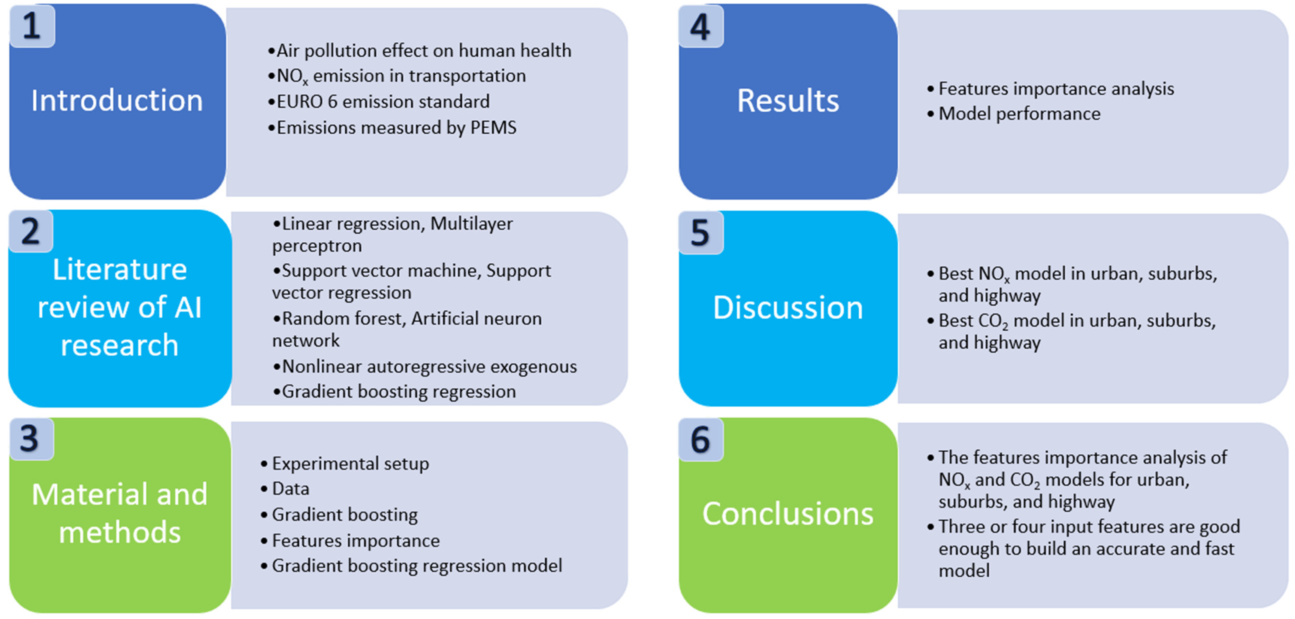
A structure diagram, Figure 1, of this article is presented to make it easier to read this paper.
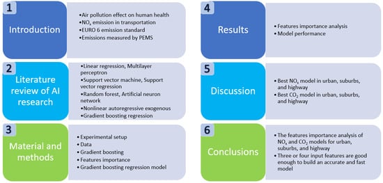
Figure 1.
Structure of this study.
2. Literature Review of AI Research
Jaworski et al. presented an analysis of emission data from the PEMS system for real driving cycles of various types of vehicles, complying with EURO 2–EURO 6 standards and created the emission models with the Regression Learner applications in MATLAB R2018b. Among the methods of regression trees and support vector technologies that have been used, the boosted regression tree model was assessed to be the most appropriate to well represent the real data [14].
Donateo et al. proposed a neural network model based on the interpolation of the time-histories of driving conditions (speed, altitude, ambient temperature, humidity, and pressure) and emissions measured on a diesel start-and-stop vehicle while performing a series of real driving emission (RDE) tests. The Bayesian optimizer, implemented in the MATLAB environment, was used to deal with the high number of combinations. This method minimized the number of combinations examined by the model and significantly reduced the computational time [15].
As mentioned above, a lot of PEMS measurements in real road driving have been conducted before, but not many of them have used artificial intelligence (AI) to analyze the collected data and to establish models for further predictions and evaluations. The purpose of this study is to investigate the technique of AI models for diesel vehicles in real road driving to reduce the cost of calculation and to increase the accuracy of the model prediction.
The big data analysis technique is an important tool to reduce the cost of emission measurements on real roads. Compared with traditional ways of data analysis, the analysis of vast amounts of data is no longer difficult in today’s big data era. For regression analysis, machine learning technology has been widely used in related topics, such as support vector machine (SVM), random forest (RF), and artificial neural networks (ANN).
Zeng et al. used SVM to estimate the fuel consumption of gasoline vehicles and found a relationship between the fuel consumption and the corresponding factors such as average speed and driving distance [16]. They also used the multiple linear regression (MLR) model and artificial neural network to link the fuel summation with the SVM model for comparisons. However, the measurement period took one month, which is too much of a cost in time.
Henrik Almer compared the effect of sampling rate on the model performance. He used the vehicle data, road data, and weather data collected in one year between 1 June 2013 and 31 May 2014 for training. The data collected between 1 June 2014 and 31 October 2014 were used for validation and testing. The results of comparison showed that the sampling rate of 10 min is better than the sampling rate of 1 min in model performance because of its smaller variance in predicting fuel consumption. Moreover, among machine learning models (linear regression, random forest, support vector regression (SVR), and ANN), the performance of the random forest model was the best [17].
L. Thibault et al. presented the use of information and communication technology (ICT) to transmit driving information to the cloud system through smartphones and to calculate pollutant emissions in real time [18]. This coupled a microscopic model with a real-world speed profile to estimate on-road pollutant emissions. However, it is not possible to use the existing microscopic model well for a large vehicle fleet because the input parameters of this model are not available for all vehicles. Thus, the modeling approach should be chosen according to the vehicle data available for each car.
Air pollution is one of the major concerns for citizens due to its impact on public health. Vehicle emissions are related to vehicle technology and driver behavior. Therefore, L. Thibault et al. created a vehicle IoT device that gives the driver real-time feedback about the emissions and reminds the driver of exposure during the trips [19]. The whole system includes an IoT device, a smartphone, and web-based simulation models. It provides a chance to improve the existing emissions through driving behavior.
Alimissis et al. used two interpolation methodologies to evaluate the ANN model and MLR model of urban air quality data. The predictions of air pollutants’ concentrations were compared with statistical measurements. ANN models were found to have better performance than MLR models in most cases [20]. G. Bandyopadhyay and S. Chattopadhyay also compared the performance of the ANN model and MLR model for ozone data. They found that ANN models are perfect for an interpolation solution to nonlinear problems using one input variable [21].
M. Gardner and S. Dorling used multilayer perceptron (MLP) neural networks to model the NOx pollutants and found that they perform well in predicting hourly variations of NOx and NO2 [22]. This indicates that MLP neural networks are capable of coping with complex patterns of source emissions.
In addition, F. Perrotta et al. proposed a big data-type analysis of the driving fuel consumption records of 1010 trucks over a 300 km travel distance, and performed a large amount of data processing using three techniques (SVM, RF, ANN) in a machine learning model [23]. They successfully established a fuel consumption model with big data and found that the RF model outperformed the other two models.
The gradient boosting regression model is a very powerful tool in modeling and prediction, and has been applied in many different fields [24,25,26,27,28]. However, this model has not been used in pollution predictions widely. A review conducted in 2018 by Bai et al. [29] showed that many AI methods have been used for air pollution predictions, including ANN, adaptive neuro-fuzzy (ANF), MLP, SVM, and SVR. However, the GBR model was not included. An investigation of the predictive power of the GBR model was carried out in this paper. Wen et al. proposed another ANN nonlinear autoregressive exogenous model (NARX) to predict NOx emissions in real road driving [30]. It is an inexpensive way of conducting RD emission measurements using an NGK NOx sensor and an Arduino board with Can Bus to measure the instantaneous vehicle emissions on the road. The results of measurement seemed to be quite reasonable compared with a full PEMS system.
Yun et al. proposed a real-time model to predict vehicle instantaneous emissions such as NOx and CO2 [31]. This is a practical model that integrates an ANN model with a vehicle dynamic model. The accuracy of both NOx and CO2 models were evaluated by varying number of features.
Table 1 summarizes the key points of previous investigations conducted by other researchers related to the AI model applications in vehicle emissions measurements.

Table 1.
Key point of each study in the literature review.
The process of this study is to establish the AI model of one vehicle based on the PEMS data of that specific vehicle in urban, suburb, and highways situations and then use the data to predict the emission and fuel consumption for the second route of the same vehicle. One vehicle was used in this study. The model performance of the vehicle includes NOx and CO2 emissions and fuel consumption.
The method of gradient boosting regression (GRB) was adopted in this study to model the NOx and CO2 emissions in three routes (urban, suburbs, and highway) and use them to predict the NOx and CO2 emissions and fuel consumption of the same vehicle on a second journey. A different number of input features were chosen for comparison to determine the best combinations of input features of the models.
3. Materials and Methods
3.1. Experimental Setup
The HORIBA OBS-ONE PEMS was used in this research for emission measurements on the real road. It is vehicle-mounted pollution analysis equipment that can be used to measure CO, CO2, THC, NOx, and PN in driving vehicles continuously. The system also integrates with the satellite positioning system (Global Positioning System, GPS) and the environmental conditions such as atmospheric temperature, humidity, atmospheric pressure, etc., to obtain the actual emissions data when the vehicle is driving on real roads. The specifications of the PEMS are listed in Table 2 [32]. There are 35 parameters that can be collected during the real road testing.
Table 2.
Specifications of HORIBA OBS-ONE PEMS [32].
The detailed settings of PEMS installation are shown in Figure 2, including the location of the analyzer, pitot tube flowmeter, atmospheric sensors, tailpipe temperature sensor, and primary control computer [10]. Figure 2 shows the installation of the system in the cabin of the test vehicle. The function of the primary control computer is using the HORIBA default software to collect the data from different sensors, store the data, and output the raw data.
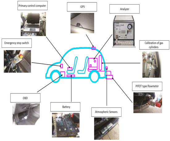
Figure 2.
Detailed settings of PEMS installation [10].
The PEMS system was powered by an independent battery pack inside the cabin. All the instruments were well grounded to the negative pole of the battery to prevent any pulse damage. Moreover, standard gases were carried in the cabin for calibration of sensors before and after each test to ensure the accuracy of measurement.
The raw data were processed in the following way. Take the NOx data as an example. The direct measurements by the PEMS system include the instantaneous concentrations of NOx in the exhaust flow (), the exhaust temperature (), the pressure in the exhaust pipe (), and the exhaust flow rate (). The density of NOx () was obtained using the equation of state for ideal gas with the exhaust temperature and the exhaust pressure. The instantaneous concentrations of NOx can then be converted to the mass flow rate by multiplying the exhaust mass flow rate as shown by Equation (1).
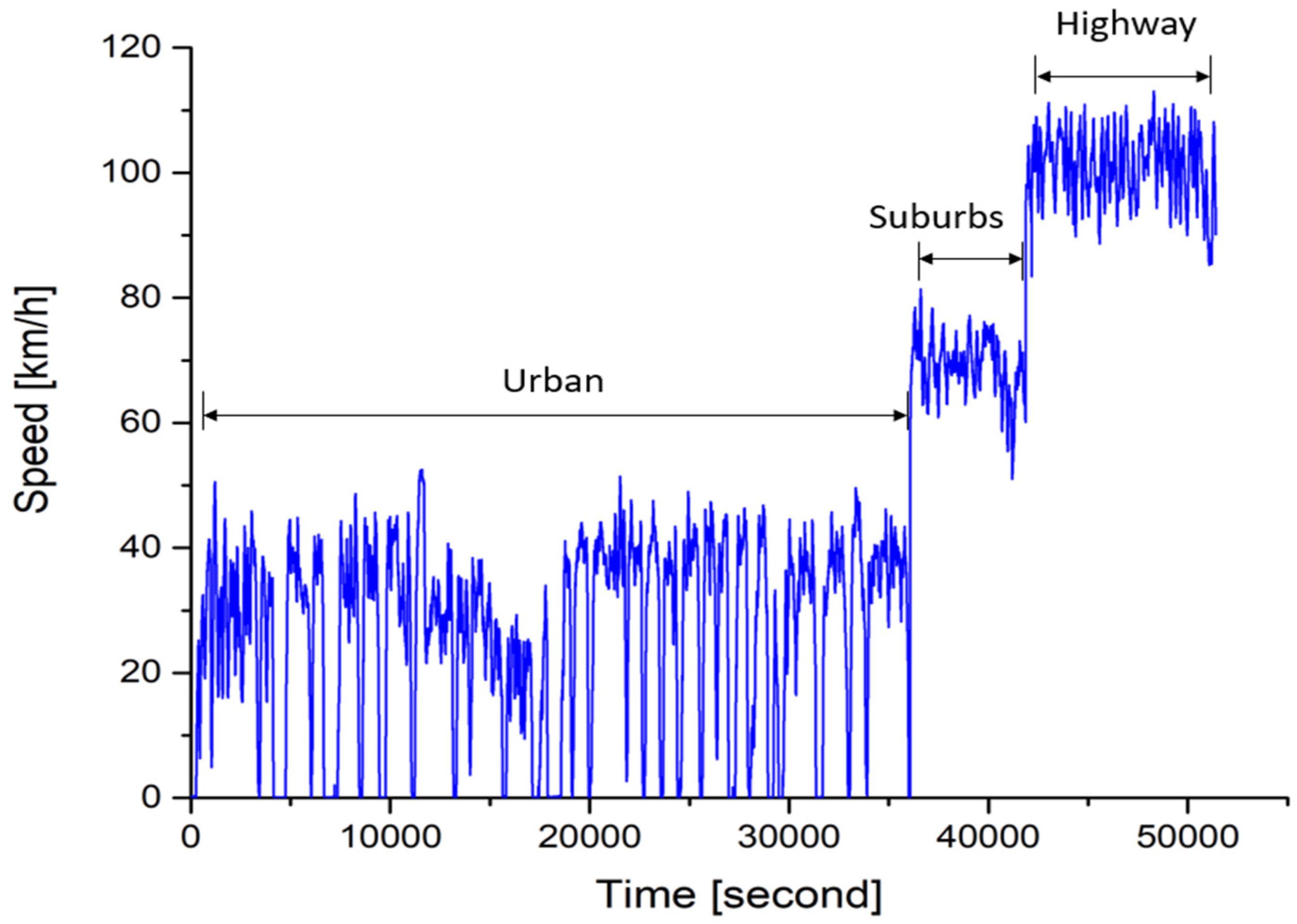
One light duty diesel vehicle, Peugeot 208, produced in 2015, which meets EURO 5 emission standards, was used as the testing vehicle in this study. The engine displacement of this vehicle is 1.6 L. The testing vehicle was run on real roads with two routes. The driving route started from Zhangbin Industrial Park to Lukang, Puyan, and Huawei. The total distance of this route is about 64 km. The route was divided into three parts intentionally, including urban, suburbs and, highways. The vehicle speed in each part was well controlled in specific ranges. The driving speed was from 0 to 60 km/h in the urban, from 60 to 90 km/h in suburbs, and above 90 km/h on highways. Figure 3 shows the speed variations of route 1. It is noted that vehicle speed varies a lot in the first part because of lots of traffic lights in the urban area. In the second part, we can see that the vehicle speed was much faster than that in the urban area. No traffic lights were observed in this part. In the last part of this route, the vehicle speed was in the range of 90~110 km/h. This is the highway part. However, the speed was not fixed in a constant value because acceleration and deceleration occurred quite often during overtaking, and the average speed was above 100 km/h.
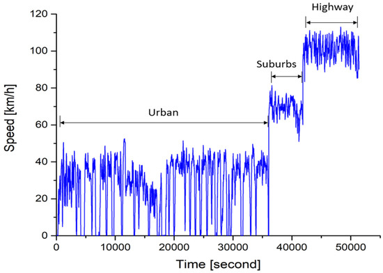
Figure 3.
Speed variations of testing vehicle in route 1 of the real road.
Two vehicle routes were used in this study. The driving patterns of these two routes are shown in Table 3. It is noted that these two routes are not different by very much. The distance and the average speed were controlled so as not to deviate from each other. The driving data on the urban, suburbs, and highways sections were analyzed in this paper. One used for building the model, and the other was used for validating the model.
Table 3.
Driving pattern of the testing vehicle on real roads.
3.2. Data
The total time span for one route was about 90 min. The sampling rate of data collection was 10 Hz. The 10 Hz sampling rate is fast enough to capture the transient behavior of the vehicle in acceleration or deceleration. A higher sampling rate is feasible for the hardware capability of the PEMS system. However, it will cause a big burden for the following data analysis because a total of 35 data were collected at a time. In total, about 54,000 data sets could be collected in one testing. There were, in total, 35 raw data collected in the PEMS. The raw data can be divided into three groups. One is operating parameters of the vehicle, including exhaust volume flow rate (m3/min), exhaust temperature (°C), exhaust pressure (kPa), engine coolant temperature (°C), fuel pressure (kPa), engine speed (rpm), intake air temperature (°C), mass air flow rate (g/s), fuel rail pressure (kPa), fuel rail pressure (direct inject) (kPa), commanded EGR (%), barometric pressure (kPa), fuel rail pressure (absolute) (kPa), engine oil temperature (°C), engine fuel rate (L/h), actual engine percent torque (%), and engine reference torque (Nm). The second group is the environmental parameters of the vehicle, including test time (s), test distance (km), GPS altitude (m), GPS latitude (deg), GPS longitude (deg), GPS speed (km/h), GPS course (deg), system battery voltage (V), ambient temperature (°C), ambient relative humidity (%), and ambient pressure (kPa). The third group is the outcome of the vehicle, including CO (ppm), CO2 (ppm), H2O (%), NO (ppm), NOx (ppm), NO2 (ppm), and THC (ppmC).
Since the goal of this research is to build the models of CO2 and NOx, some parameters that are not closely related to the formation of CO2 and NOx are not considered in this study to reduce the burden of model building.
The instantaneous NOx and CO2 concentrations in the tailpipe are shown in Figure 4a,c. The raw data were recorded with a sampling rate of 10 Hz. A total of about 36,070 data are presented in this Figure. It is noted that the NOx concentrations in the urban part vary a lot at different vehicle speeds. The same trend could be found in suburbs and highways. Even on the highway, the vehicle speeds are quite stable, and the NOx concentrations vary a lot too. The variations of CO2 concentrations are similar to NOx emissions mentioned above. The maximum values of CO2 are about 120,000 ppm (12%), which corresponds to an air–fuel ratio of about 20 at full loads. The minimum values of CO2 are about 1093 ppm, which corresponds to very lean combustion at idle condition. It is noted that the CO2 concentrations of diesel engines are much lower than of gasoline counterparts because diesel engines run at much leaner conditions [33].
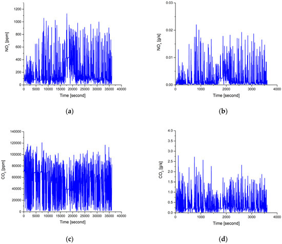
Figure 4.
The instantaneous concentrations and the production rates of NOx and CO2 in urban part. (a) NOx concentrations (ppm); (b) NOx production rates (g/s); (c) CO2 concentrations (ppm); (d) CO2 production rates (g/s).
The instantaneous concentrations can be converted to the mass flow rate by multiplying the exhaust mass flow rate by Equation (1). The results of the conversion calculation are shown in Figure 4b,d. Because of the limited space, only the variations in urban area are shown. It is noted that the maximum flow rate of NOx is about 0.022 g/s, which occurs at acceleration. The minimum flow rate of NOx is about 0.00004 g/s, which occurs at deceleration. For CO2, the maximum flow rate is about 2.79 g/s, which occurs at acceleration, and the minimum flow rate is about 0.0068 g/s, which occurs at deceleration.
The instantaneous flow rate can be integrated with time to obtain the total emission production factor. The results of the integration are shown in Table 4.
Table 4.
Total emission rate.
3.3. Gradient Boosting
An introduction of gradient boosting was presented by Li [34]. This indicated that the gradient boosting consists of two sub-terms, gradient descent and boosting, and it could be applied in regression, classification, and ranking. These applications are based on the gradient boosting algorithm proposed by Friedman [35]. This algorithm is used to minimize the loss function of the model by adding weak learners using gradient descent. The regression function is shown in Equation (2). The ensemble of gradient boosting is a supervised learning algorithm that can learn nonlinear functions to solve regression and classification problems. It is a complex model built by combining several simple models in the best possible way. The high bias and low variance models can be combined additively to form an ensemble with reducing bias while maintaining the low variance in boosting.
where is the loss function and is the base-learner model. For each iteration m = 1, 2, ⋯, M, compensating the residues is equivalent to optimizing the expansion coefficients and .
3.4. Features Importance
There are 35 parameters that were collected by the PEMS during the RD testing. Nine of them are closely related to the formation of NOx, and they are considered as the input features for the NOx model, including mass air flow rate (g/s), exhaust flow rate (m3/min), CO2 (ppm), engine speed (rpm), tailpipe exhaust temp (°C), GPS speed (km/h), ambient humidity (%), ambient temperature (°C), and GPS altitude (m). As for the CO2 model, eight input features were considered for building the model, including exhaust flow rate, mass air flow rate, engine speed, GPS speed, tailpipe exhaust temperature, ambient humidity, GPS altitude, and ambient temperature.
Since there are too many input features for the NOx model as well as the CO2 model, a way of reducing input features should be considered to reduce the calculation burden. John et al. proposed the two main categories of reducing selected feature numbers [36]. One is the wrapper method that pluses and/or reduces the features to figure out the optimizer that could obtain the highest performance. The other is the filter method that evaluates the correlation between the variable and the predicted value, and excludes the least relevant variable.
Casimir et al. used the Sequential Backward Selection (SBS) algorithm to find the most relevant features [37]. The appropriate features are determined for better accuracy. Dewi et al. proposed a method to cope with the features selection by using random forest (RF) algorithm [38]. They found out that different combinations of features created different model accuracy. As a result, the model performance is higher after using the RF features selection algorithm. The model performance statistic results of using four datasets (Wisconsin Cancer, Forest Fire, Wine Quality, and Bike Sharing) show that more input features do not guarantee obtaining higher performance because more features add more complexity to the model.
There are ten features (nine features from PEMS and acceleration derived from GPS speed) that were selected for the NOx model and nine features (eight features from PEMS and acceleration derived from GPS speed) for the CO2 model. The rank and score of feature importance were generated by permutation techniques. This was written in python code by importing the permutation_importance from sklearn library directly. The results showed their relative predictive power to the model. The process is used to break the input feature values by randomly shuffling. This step might decrease the model performance. If the decrease is small, it means the performance of the model is pretty good. Furthermore, if the decrease is large, there is a large impact on predictions.
3.5. Gradient Boosting Regression Model
Python is an interactive, object-oriented programming language. It has hundreds of excellent libraries for developers to use. Python offers a programming language that is stable, flexible, and has tools available. Therefore, there are lots of Python AI applications today. The GBR model was built in Python code. The coding process includes preprocessing, data-loading, model-defining, and model-fitting.
In this study, the data are divided into two subsets, the training set and the testing set for building the GBR model. The percentage of each data set is listed in Table 5. In general, the train–test split procedure is used to estimate the performance of the model. In this study, the training data are 75%, and the testing data are 25%.
Table 5.
Training and test sets.
In building the GRB model, several parameters should be assigned in the beginning. The main parameters for the NOx model are listed in Table 6. The parameters of the GBR model include the following: N_estimators denote the number of trees used for boosting, and the default value is 100. Its value was set at 500 in this model. More estimators may obtain better model performance but require more calculation cost. Max_depth denotes the maximum depth of the tree, and the default value is 3. It was set at 12 in this code. Min_samples_split denotes the minimum number of samples needed to split an internal node, and it was set to 10. Max_features denote the number of features to consider when finding the best split, and the number is the square root of total features. The subsample denotes the fraction of samples that can be used to fit the individual base learners, and the default value is 1.0. Its value was set at 0.8 in this model. Learning_rate denotes a learning rate that determines the step size at each iteration while moving toward a minimum of a loss function and the value was set at 0.1. Loss denotes the loss function. Ls was selected in this code and meant the least square loss function. There is another loss function that can be selected such as lad (least absolute deviation), huber (combination of ls and lad).
Table 6.
GBR model parameters.
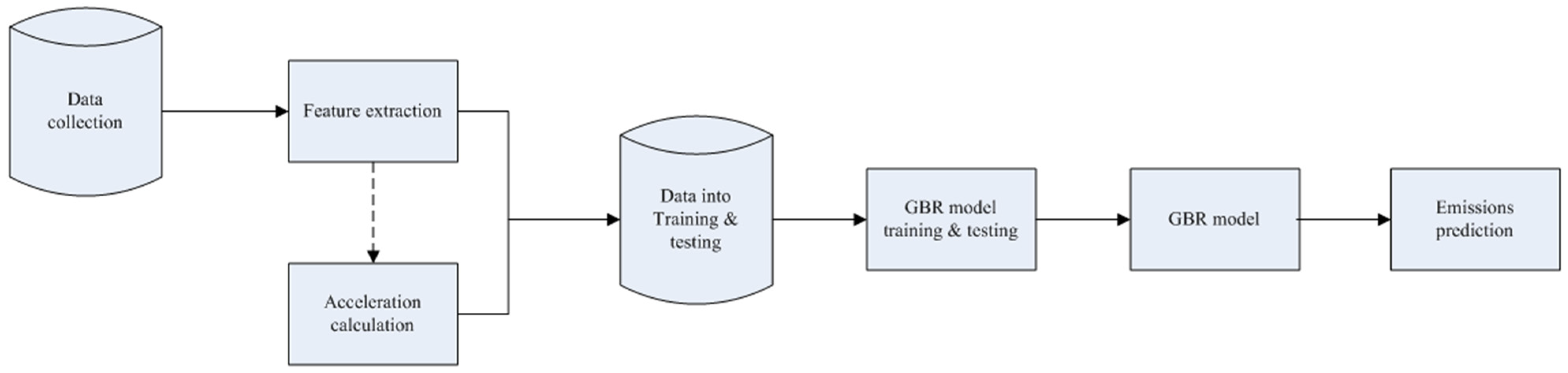
During the training process of the GBR model, the ensemble was imported from Python module sklearn (SciKit-Learn) and using the gradient boosting regressor defined with an ensemble. The GBR model was defined with the above parameters and was used to fit the experimental data. Figure 5 shows the flowchart of the proposed method for emissions prediction. The first step is collecting data from PEMS records. Then, feature extraction is conducted that uses the features selection method to determine the appropriate features for model input. It is noted that acceleration is not the raw data collected by PEMS directly. It needs to be calculated from the GPS speed. The third step is loading the data and splitting them into training and testing sub-datasets by fraction. Then starts the process of training and testing for the model. The fifth step is finishing the compile process and obtaining the model. Finally, the model is used to predict the emissions in the second route.
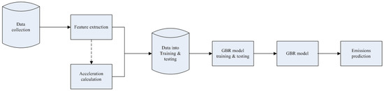
Figure 5.
Flowchart of proposed method for emissions prediction.
The model performance is examined by using mean absolute error (MAE), root means square error (RMSE), and the coefficient of determination . The statistical equations are given in Equations (3)–(5), respectively, where Pi is the predicted value obtained with the model and Ti is the measured value from PEMS. is the average of the predicted value for the whole dataset.
4. Results
4.1. Features Importance Analysis
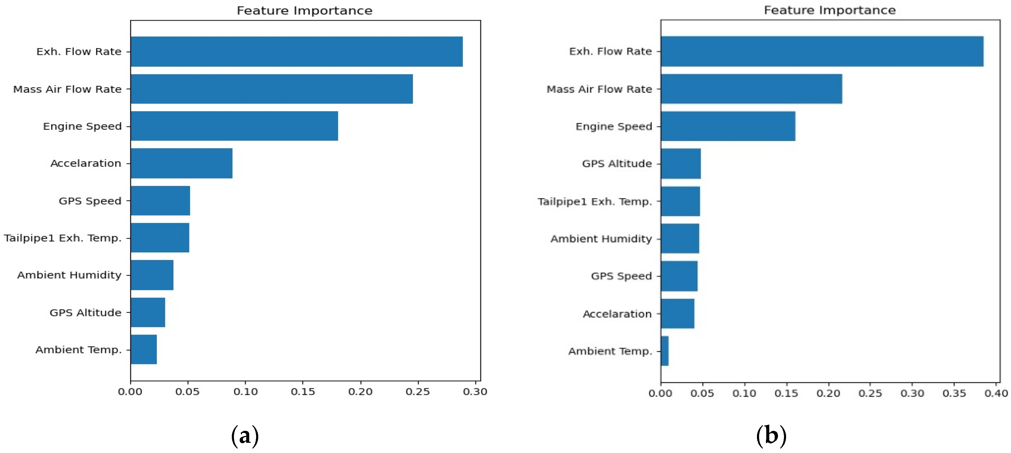
The detailed scores ranking of feature importance for NOx models in the urban, suburb, and highway driving patterns are shown in Figure 6. It is noted that the top three features of NOx models are the same for urban, suburban, and highways. They are mass air flow rate, exhaust flow rate, and the concentration of CO2. It is not surprising that mass air flow rate is the most important feature because it is closely related to engine load, and NOx formation is known to be dominantly determined by engine load. The second important feature is exhaust flow rate, which is actually the sum of mass air flow rate and mass fuel flow rate. Air–fuel ratio is also known to be an important factor to determine the formation of NOx. No wonder it is the second important feature. The third important feature is the concentration of CO2 in the exhaust flow. CO2 is one of the products of combustion, just as NOx. However, unlike the gasoline engine in which CO2 concentration in the exhaust flow is almost a constant value, the concentration of CO2 in diesel engines reflects the air–fuel ratio as well as the engine load. As a result, the CO2 concentration is also a good feature for the NOx model.
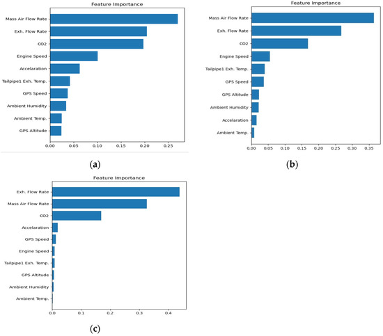
Figure 6.
Feature importance detailed scores of NOx model (a) Urban; (b) Suburbs; (c) Highway.
The fourth important feature in the urban, suburb and highway patterns is not the same for all. It is interesting to note that engine speed is important in urban and suburbs driving, while acceleration is important on the highways. Engine speed is related to vehicle speed. We can see that vehicle speed varies a lot in both urban and suburbs driving, as shown in Figure 6. However, the vehicle speed is almost fixed in a narrow range on highways. That is the reason engine speed is not so important on highways.
All of the other features are not important relative to the first four features. The order of importance of the last six features in urban, suburb, and highways patterns are not the same either. Since the importance of the last six features is much lower than the first four, the order of these features is actually not to be discussed in this study.
Table 7 shows the ranking of all features in urban, suburbs, and highways driving again for a clear comparison. It is noted that even though the actual order of the last six features is not exactly the same, the trend of descending of the order is quite similar. It could be concluded that the relative importance of the features of the NOx model in urban, suburban, and highways driving are quite close to each other.
Table 7.
Feature importance rank of NOx model in urban, suburbs, and highway.
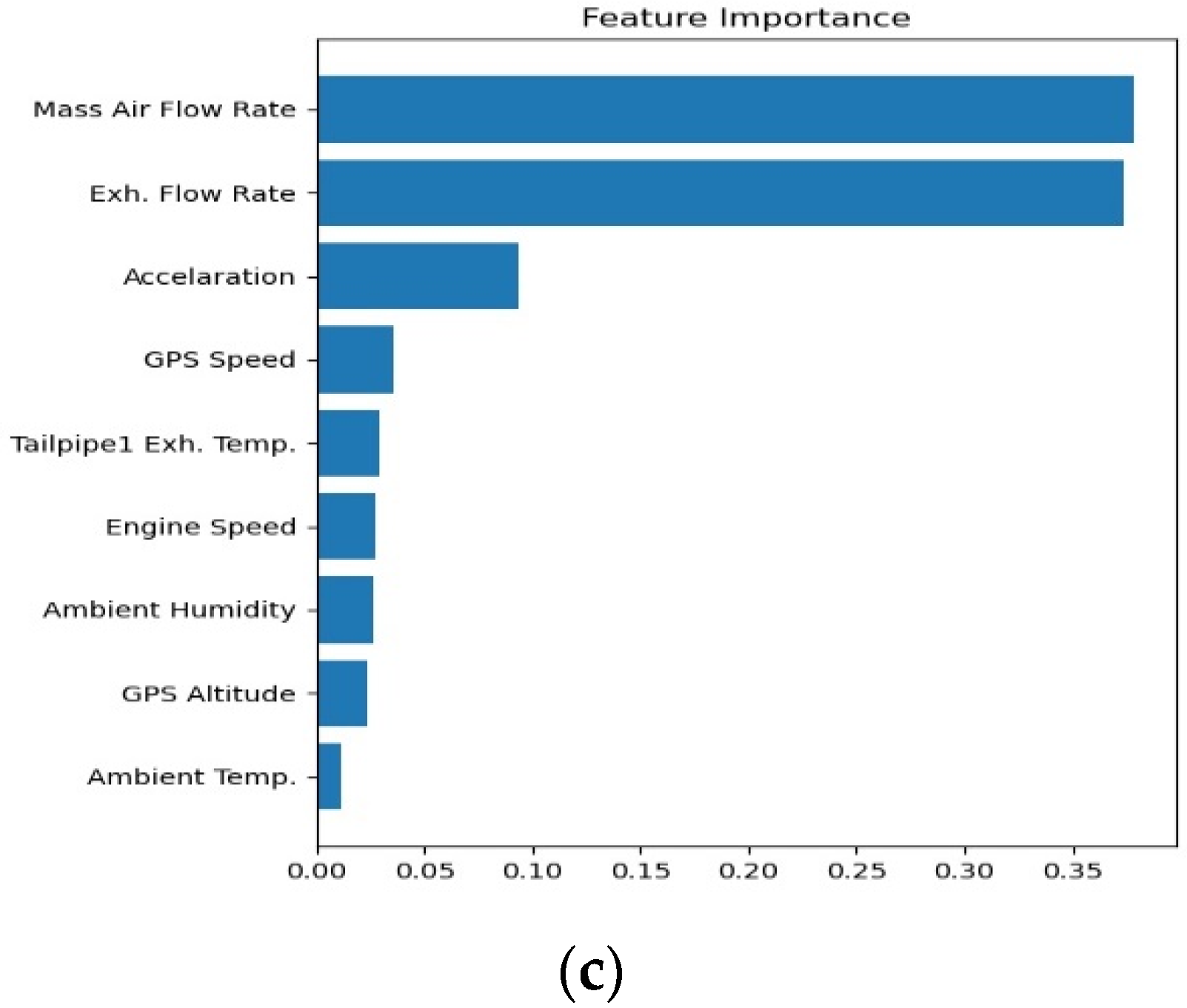
The number of features is nine for the CO2 model. All of the features are the same as the NOx model, except that CO2 is excluded. The ranking of feature importance of CO2 models for urban, suburbs, and highways patterns are shown in Figure 7. It is noted that the top two features of CO2 models are the same for urban, suburban, and highways driving. They are mass air flow rate and exhaust flow rate. This is reasonable because these two features are closely related to engine load and air–fuel ratio, and the CO2 concentration is determined by air–fuel ratio, while the CO2 production rate is determined by engine load.

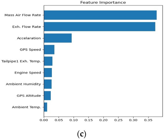
Figure 7.
Feature importance detailed scores of CO2 model (a) Urban; (b) Suburbs; (c) Highway.
The third important features in urban, suburbs and highways are not the same. It is interesting to note that engine speed is important in urban and suburbs driving, while acceleration is important in highways, just as was the case in the NOx model. The reason is also the same. Vehicle speed varies a lot in both urban and suburbs driving, but it is almost fixed in a narrow range in highways driving. That is the reason engine speed is not so important on highways.
Nine input features were considered in the CO2 model. However, not every feature is important for prediction. According to our calculation, the importance of each feature is ranked in Table 8. It is noted that the order of relative importance is not the same in the urban, suburbs, and highways driving patterns. Table 8 shows the ranking of all features in urban, suburbs, and highways again for a clear comparison. The first three features contribute the most (above 70%) importance from Figure 7. This also means the other six features contribute to a lesser extent. It is noted that even though the actual order of the last six features is not exactly the same, the trend of descending of the order is quite similar. It could be concluded that the relative importance of the features of the CO2 model in urban, suburbs, and highways driving are quite close to each other.
Table 8.
Feature importance rank of urban, suburbs, and highway CO2 model.
4.2. Model Performance
In this study, ten input features and nine input features were selected for NOx and CO2 models, respectively, and the targets were NOx emission gram per second (g/s) and CO2 emission gram per second (g/s). The statistics of model performance for NOx and CO2 in the three parts of route 1 are listed in Table 9 and Table 10. The R2 value is an important index to determine how well the model fits the raw data. The feature importance rank shown in Table 7 and Table 8 is used to check the fitting of the model. It is noted that the feature importance rank of urban driving was selected as the base, and the same order was used in suburbs and highways. It is found that for the NOx model, the R2 values of train data are all very close to 1.0 in all three parts of route 1. As for the test data, the R2 values of the urban part increase from 0.78 to 0.98 as the number of features increase from 3 to 10. The more input features we use, the higher value of R2 we have. It is a reasonable result since more features are used to model the raw data, it is expected that more characteristics of data can be captured. However, it is worthwhile to note that there is a big gap between three features and four features, and the R2 values vary very little as feature numbers increase more. This implies that four features are the minimum number to totally grasp the characteristics of NOx in the urban area. In the suburbs part and the highways part, the same trends of R2 values occur. The gap between three features and four features is not so big as that in urban and in highways, but it is still obvious that four features are the minimum number to totally grasp the characteristics of NOx in the suburbs area and in the highways area.
Table 9.
Performance R2 statistics results of NOx model.
Table 10.
Performance R statistics results of CO2 model.
The performance of CO2 models is similar to that of NOx models. The R2 values of train data are all very close to 1.0 in all three parts of route 1, implying that the training process goes very well. As for the test data, the R2 values of the urban part increase from 0.80 to 0.95 as the number of features increase from three to nine. However, unlike the NOx model where a big gap between three features and four features can be observed, the R2 values increase almost linearly with the number of features up to seven features where the increase in the R2 value begins to slow down. In the suburbs part and the highways part, the same trends of R2 values occur. The R2 values increase linearly with the number of features up to six or seven features. It seems that the CO2 model needs more input features to totally grasp the characteristics of raw data in all parts of the route.
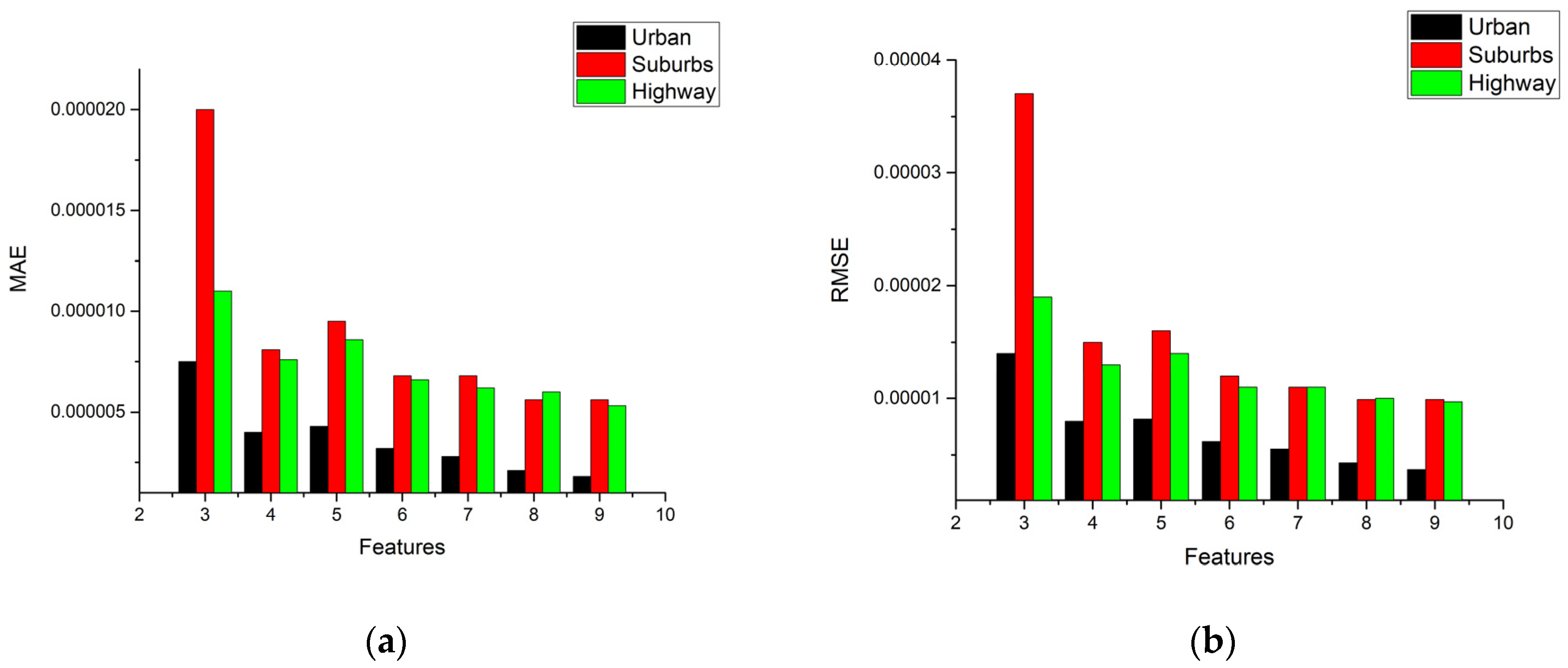
In addition, Figure 8a,b show the performance statistics results of MAE and RMSE for NOx models in route 1, respectively. They are other methods of performance evaluation used to check the model accuracy. An opposite trend of the R2 value is found, that the more features we use, the lower value of MAE we obtain. A lower value of MAE means better accuracy by the definition of MAE in Equation (3). It is noted that the prediction values are very close to the target values. In the meantime, the results for RMSE statistics are very similar to those of MAE.
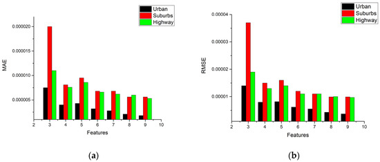
Figure 8.
Performance MAE and RMSE statistics results of NOx model (a) MAE; (b) RMSE.
In Figure 8a, it is noted that the value of MAE decreases as the number of features increases in urban, suburbs, and highways routes. Four features might be the best choice for this case considering the computational cost and accuracy, but for reaching the best performance, all features are the only option, even when using more calculation cost. It is noted that the trend in Figure 8b is the same as MAE.
Figure 9 shows the MAE statistics for the CO2 model. Only the MAE statistics are shown because the trend of RMSE statistics is also very similar to that of MAE, just as the case of the NOx model. It is interesting to note that the trend of MAE in the urban part is the same as that in the NOx model, i.e., the value of MAE decreases as the number of features increases. However, in the suburbs and highways parts, different trends show that three features input has a lower value of MAE than four features input. As a result, using three features would be the best choice to obtain good performance and low computation cost for urban, suburbs, and highways driving in route 1. Increasing the number of features can obtain better performance if computational cost needs are not to be considered. In that case, eight features might be the best choice.
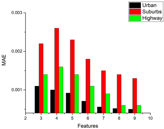
Figure 9.
Performance MAE statistics results of CO2 model.
In this study, the NOx and CO2 models obtained in route 1 were used to predict the vehicle emissions driving in the urban, suburbs, and highways parts of the second route to investigate the universality of the models. The results of NOx predictions in the second route are listed in Table 11. It is noted that the R2 values in the urban part vary from 0.69 to 0.88. The R2 values of route 2 are lower than route 1, even for the same vehicle. This is reasonable because the traffic flow, route conditions, and driver behaviors are different. The average speed of these two routes is quite similar, as shown in Table 3, but the acceleration of these two routes are different. The second route has wider acceleration ranges than route 1, probably reflecting the characteristics of the drivers. Taking a close look at the model performance, the lowest R2 value occurs when using the top three features for input features. This is the same trend as for the route 1 urban NOx model. Unlike route 1’s urban performance results, the maximum R2 values were found using six and seven features for input, and the whole results show that the performance does not increase while the number of features increases.
Table 11.
Performance statistics results of using NOx models to predict the second route NOx emission.
In the suburbs part of the second route, the range of R2 varies from 0.79 to 0.89 and shows a different trend to the urban part. The maximum R2 value uses five features for input, and then the R2 values drop after five features and reach the lowest value when using all features for input. The R2 of the highways part varies from 0.93 to 0.96. All of these values are higher than the urban and suburbs values. It is noted that the R2 of highways is the best among the three driving patterns.
The performance results when using route 1 CO2 models to predict the second route CO2 are listed in Table 12. The performance value increases while using three and four input features and reaches the maximum value of using five features, then drops with an increasing number of features for urban driving. The trend of R2 variations agrees with the results of the CO2 models feature importance analysis shown in Figure 7a. It is noted that the features importance influences the model performance a lot and reflects the same trend of using this model to predict the second route.
Table 12.
Performance statistics results of using CO2 models to predict the second route CO2 emission.
According to the above results, GBR models present excellent R2 values, representing the model performance for NOx and CO2 prediction.
Table 12 shows that the R2 values of suburbs driving are higher than for urban. This is the same result as using the route 1 NOx model to conduct prediction in the second route due to the similar feature importance, such as mass air flow rate, exhaust flow rate, and engine speed. It is interesting that the trend of R2 values of highway driving using three, four and five features are similar to urban, but the R2 values of highway driving using six, seven and eight features are similar to suburbs.
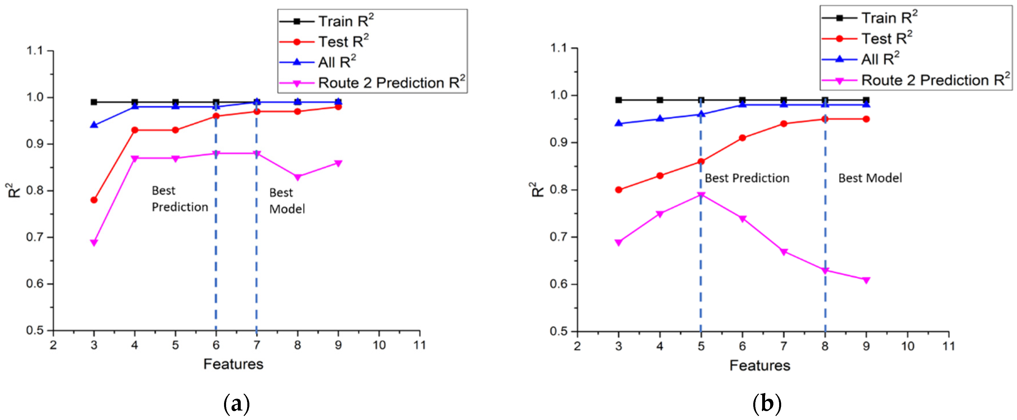
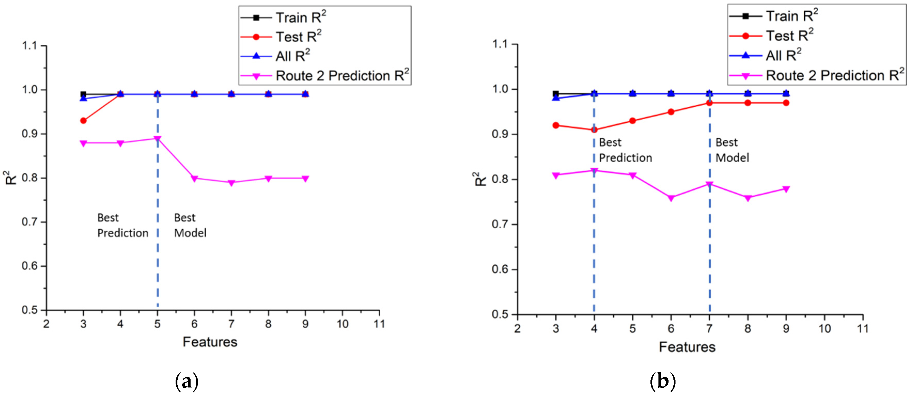
In summary, Figure 10, Figure 11 and Figure 12 shows the comparisons of the R2 values of NOx and CO2 models for the training sub-dataset, the test sub-dataset, all data, and the prediction of the second route using a different number of features in urban, suburbs, and highways according to Table 9, Table 10, Table 11 and Table 12. The criterion for the best model is to obtain the highest R2 value in both route 1 and the second route. The best prediction is the highest R2 value of the second route. For example, the best NOx model in urban driving, as shown in Figure 10a, is the model with seven input features. However, the best prediction is the model with six input features. Figure 10b shows the best model with eight input features and the best prediction with five input features for the CO2 model in urban driving, according to the same criterion. The statistics of the input number of features for the best model and best prediction in urban, suburbs, and highways routes are listed in Table 13. It can be found that the number of input features for the best prediction is less than that of the best model.
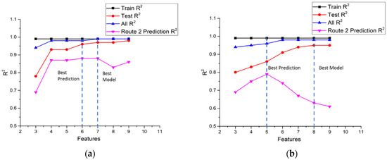
Figure 10.
(a) Comparisons of the R2 value of NOx models for the training sub-dataset, the test sub-dataset, all data, and the route 2 prediction in urban; (b) Comparisons of the R2 value of CO2 models for the training sub-dataset, the test sub-dataset, all data, and the route 2 prediction in urban.
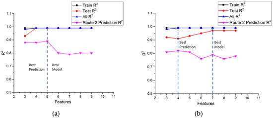
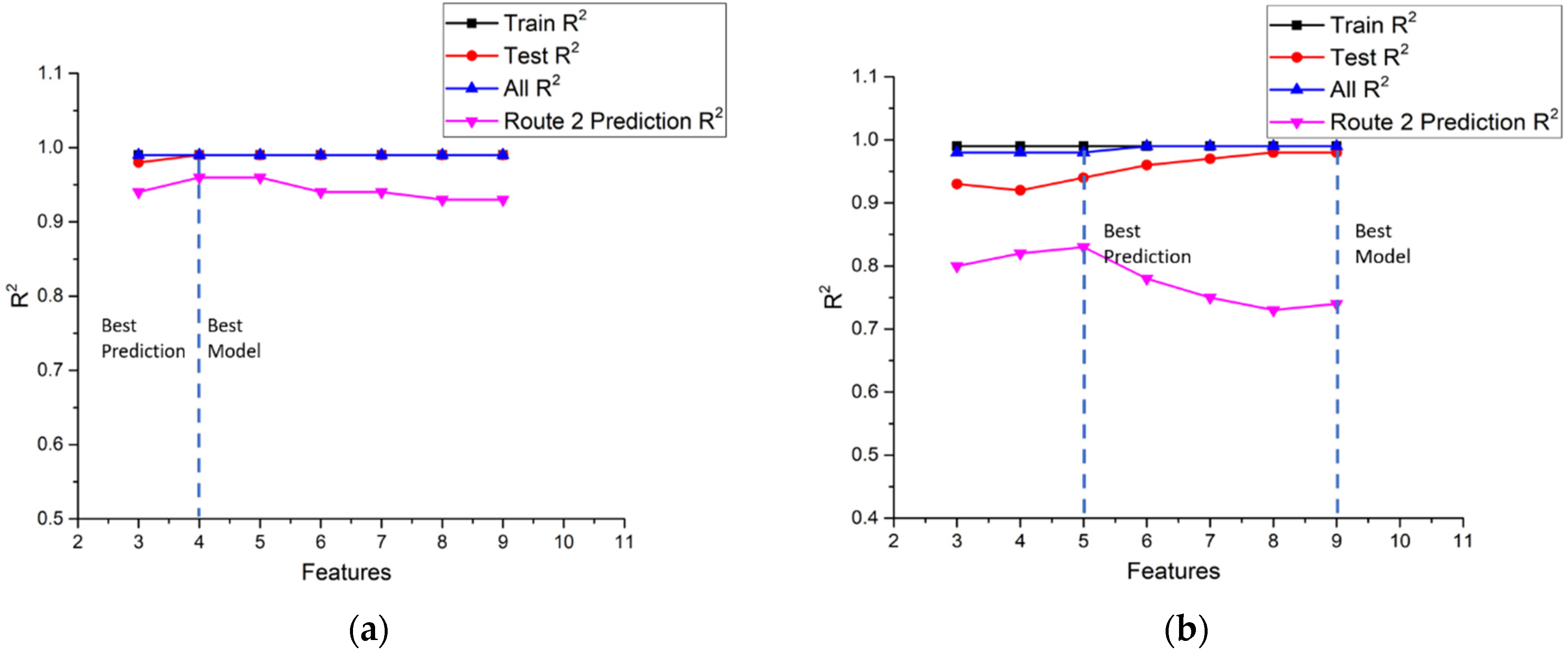
Figure 11.
(a) Comparisons of the R2 value of NOx models for the training sub-dataset, the test sub-dataset, all data, and the route 2 prediction in suburbs; (b) Comparisons of the R2 value of CO2 models for the training sub-dataset, the test sub-dataset, all data, and the route 2 prediction in suburbs.
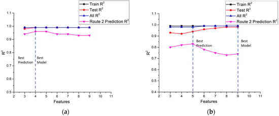
Figure 12.
(a) Comparisons of the R2 value of NOx models for the training sub-dataset, the test sub-dataset, all data, and the route 2 prediction in highway; (b) Comparisons of the R2 value of CO2 models for the training sub-dataset, the test sub-dataset, all data, and the route 2 prediction in highway.
Table 13.
Input number of features for best model and best prediction.
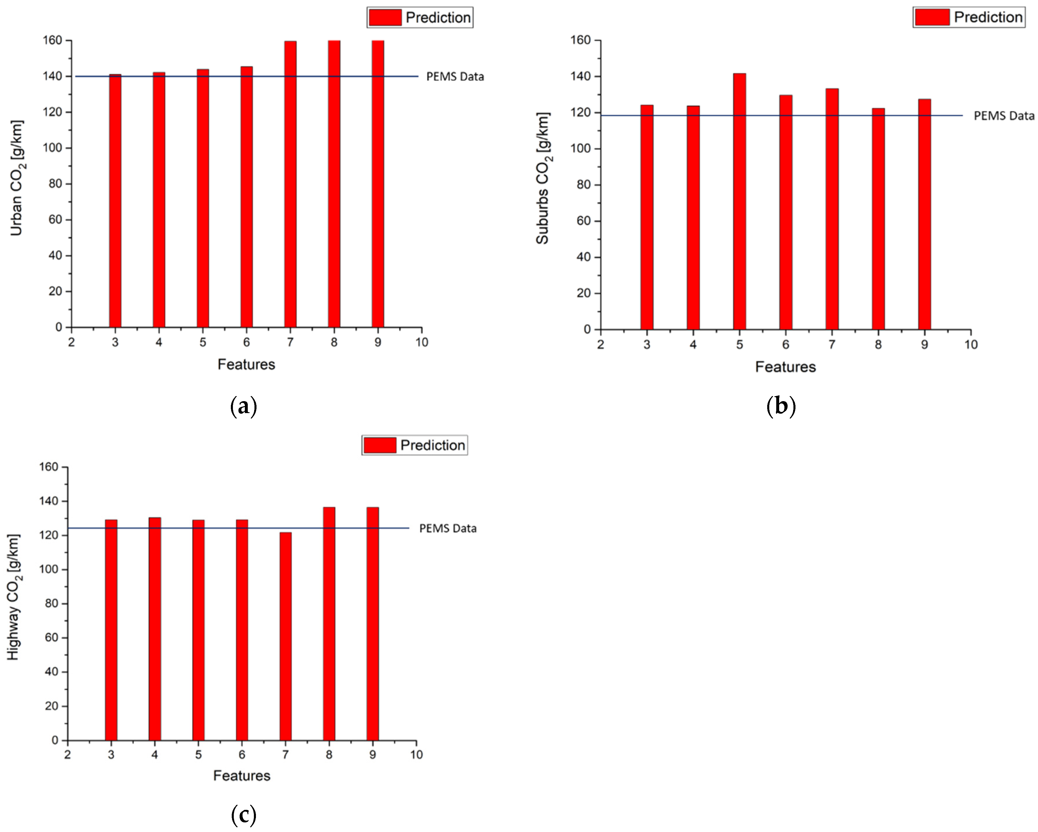
The models trained by GBR can not only predict the instantaneous emission production on the road, as shown in previous figures, but also can be used to evaluate the emission factors of the vehicle driven on real roads. Table 14 and Figure 13 present the results of the calculation for the NOx emission factors with different input features. It is noted that the predicted emission factors are very close to the measured factors in the three parts of route 1 for all the cases of 3 input features to 10 input features.
Table 14.
Results of NOx and CO2 emission factor predictions.
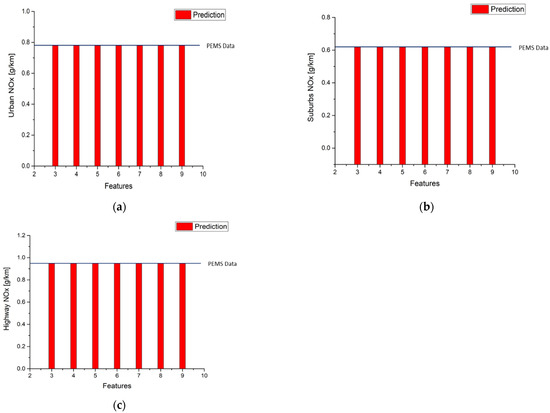
Figure 13.
Results of NOx emission factor predictions (a) Urban; (b) Suburbs; (c) Highway.
Table 14 and Figure 14 show the results of CO2 emission factors calculations. The results are as good as those for NOx predictions except in the suburbs part with six input features where the error between the predicted value and measured data is 0.4%, which is still very small.
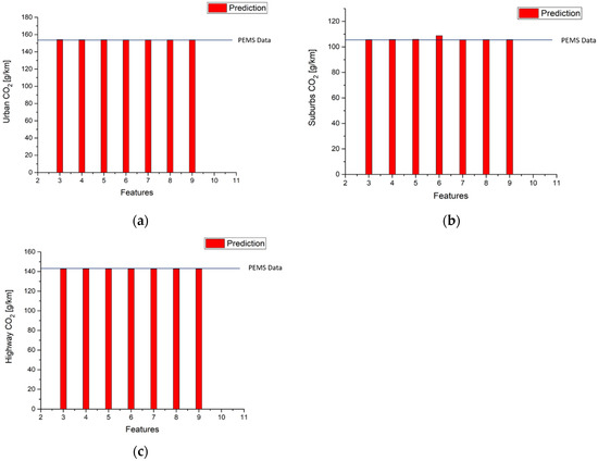
Figure 14.
Results of CO2 emission factor predictions (a) Urban; (b) Suburbs; (c) Highway.
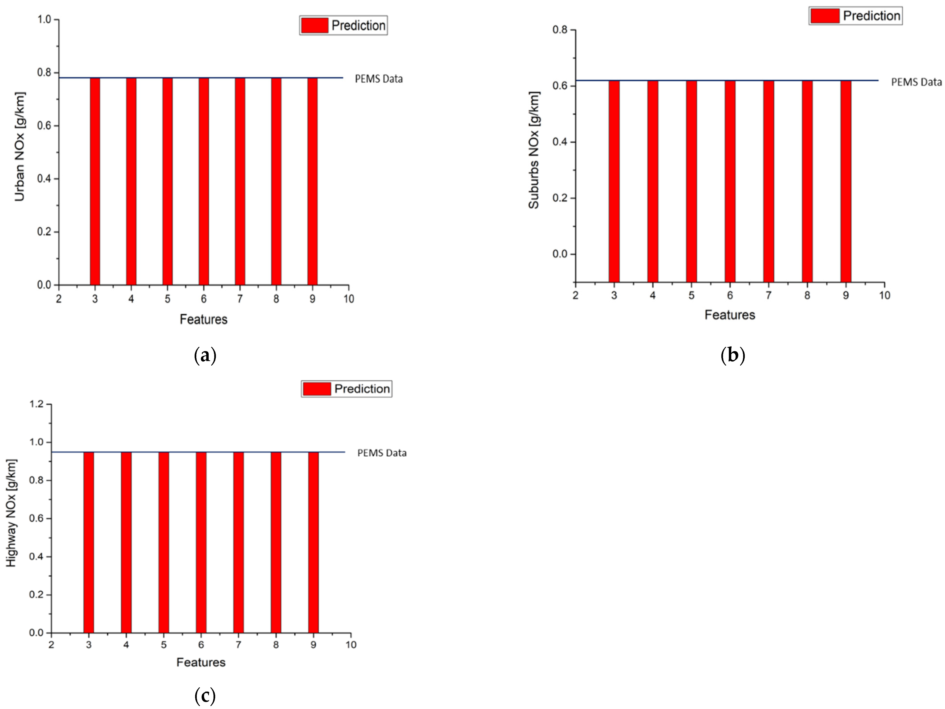
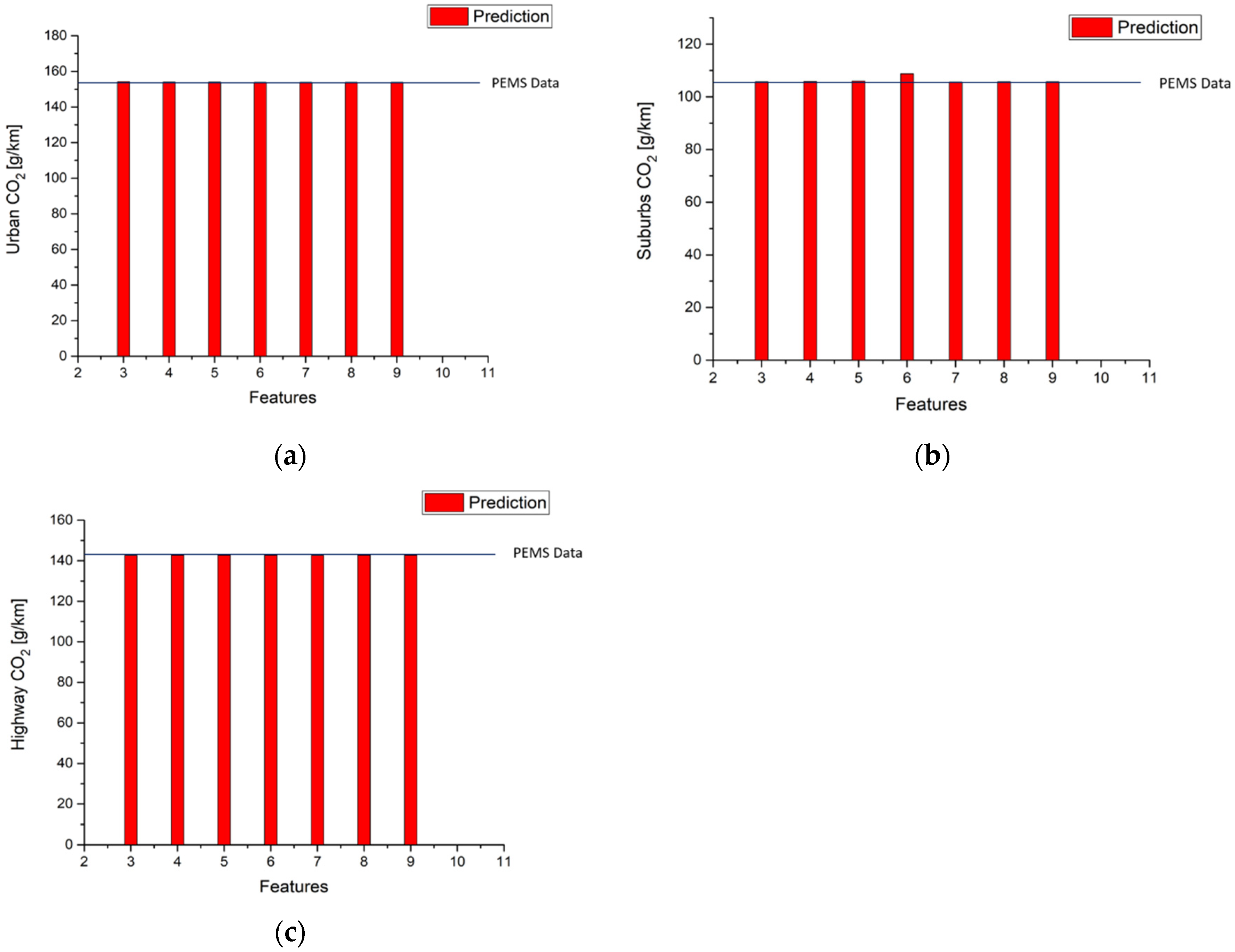
Table 15, and Figure 15 and Figure 16 show that using route 1 NOx and CO2 models to predict urban, suburbs, and highway emissions in the second route obtains the same results as Table 11 and Table 12 in terms of emissions gram per kilometer. It is clear that model performance decides the error between measurement data and predictions. The best performances of NOx and CO2 in the second route urban model use the top six features and top five features, respectively. The best performance of NOx prediction in the second route in the suburbs uses the top five features but CO2 prediction uses the top four features. The best performance of the NOx prediction in the second route in the highway model uses the top four features, and using the top five features to fit the model obtains the best performance of CO2 prediction in the highway model.
Table 15.
Second Route NOx and CO2 emission g/km predictions statistics results of using route 1 urbanmodels.
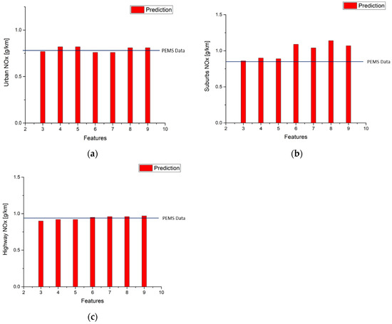
Figure 15.
Second route NOx emission factor predictions by using route 1 NOx urban model (a) Urban; (b) Suburbs; (c) Highway.
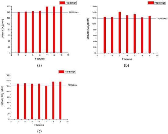
Figure 16.
Second route CO2 emission factor predictions by using route 1 using CO2 urban model (a) Urban; (b) Suburbs; (c) Highway.
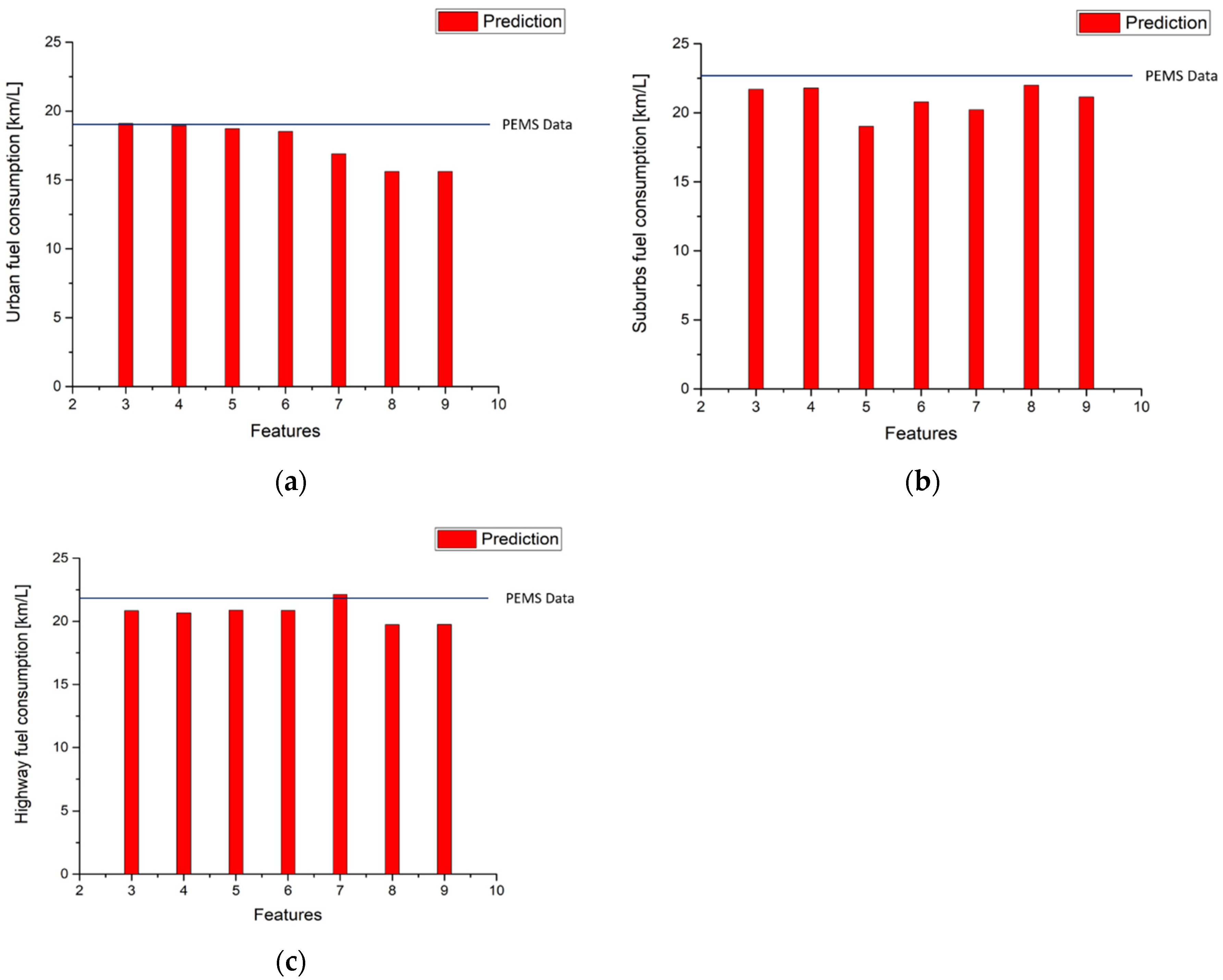
Diesel is a volatile substance that consists of hydrocarbon. The diesel fuel chemical formula is with the density of 0.85 kg/L. The stoichiometric combustion reaction of diesel fuel with air in a diesel engine is as following.
According to Equation (6), fuel consumption can be calculated by utilizing CO2 emission gram per kilometer, as obtained above. The results of fuel consumption calculations in route 1 are shown in Table 16 and Figure 17. It is noted that the errors of fuel consumption are very similar to the errors of CO2, as in Figure 12. This is very reasonable because the fuel consumption in a diesel engine is closely related to CO2 production. The results of fuel consumption predictions in the second route are shown in Table 16 and Figure 18. The same trends of model errors can be observed as in Figure 16.
Table 16.
Fuel consumption km/L statistics results of route 1 and route 2.
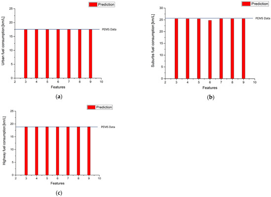
Figure 17.
Fuel consumption statistics results in route 1 (a) Urban; (b) Suburbs; (c) Highway.
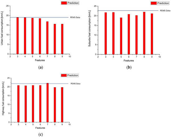
Figure 18.
Second route fuel consumption predictions by using route 1 CO2 urban model (a) Urban; (b) Suburbs; (c) Highway.
5. Discussion
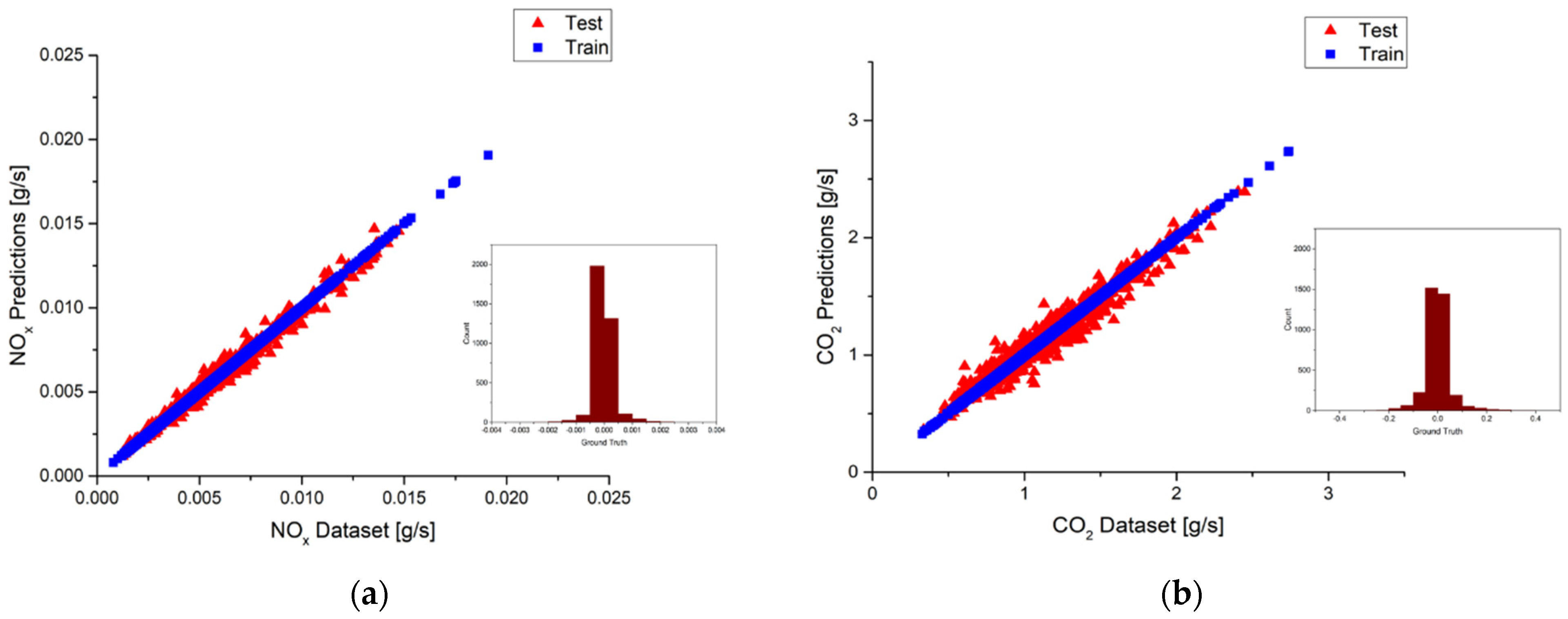
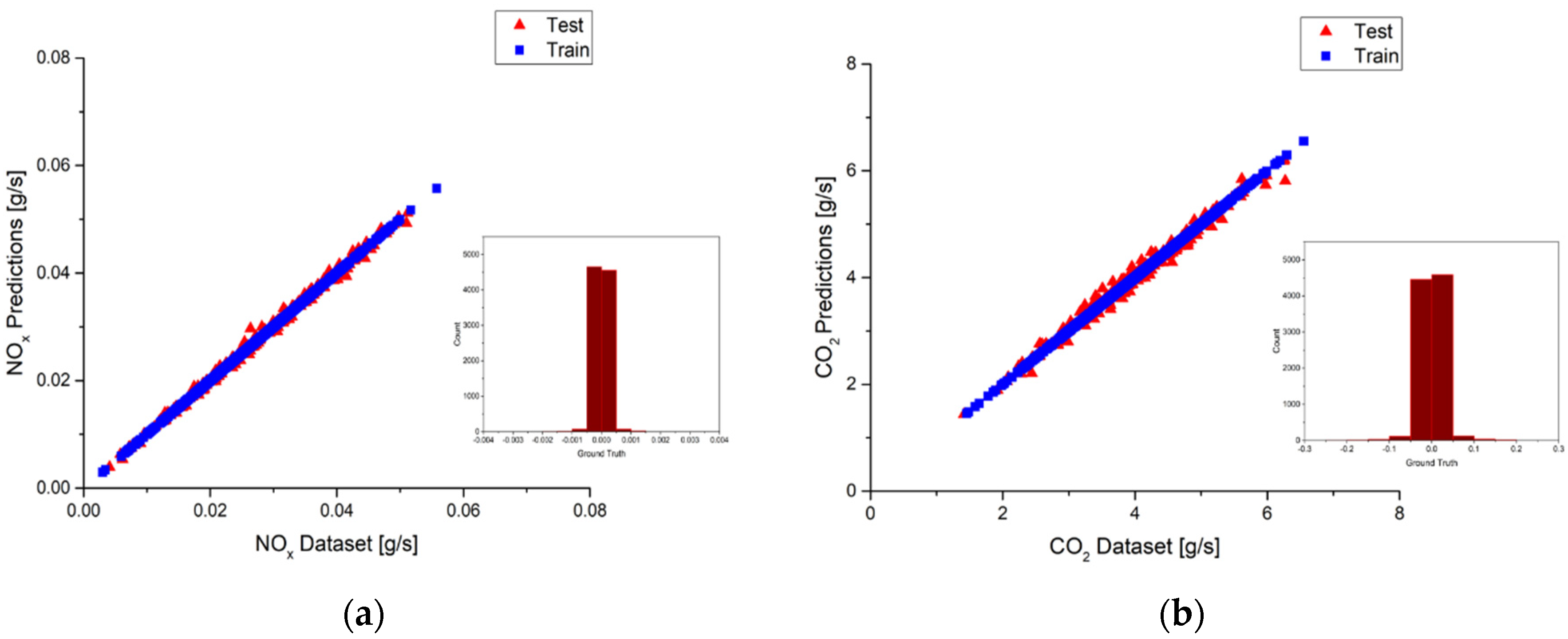
According to Table 9 and Table 10, the best model is built by selecting the top seven input features for the NOx model and the top eight input features for the CO2 model in urban driving. The R2 values of the NOx model and the CO2 model are 0.99 and 0.98, respectively. These results are the best R2 values among the NOx and CO2 models when selecting different input numbers of features. It is noted that the choice was based on the prediction accuracy only, calculation cost was not considered. The prediction results of the best NOx and CO2 models are plotted in Figure 19a,b, in which the red triangle represents the test sub-dataset and the blue square represents the training sub-dataset. Since the R2 value of the test sub-dataset for the best NOx model is 0.97, some small deviations between the predictions and the measurements can still be observed in Figure 19a. Furthermore, the bar chart located at the lower right corner shows the ground truth of the predictions. Ground truth is an evaluation of the results of model accuracy against the targets. The distribution of ground truth would concentrate on zero value for a perfect model. It can be seen for the best NOx model the distribution of ground truth spreads a little bit around zero value, indicating the existence of deviations. Figure 19b shows the predictions of the best CO2 model. The same deviations can be observed as those in the NOx model. However, since the R2 value of the test sub-dataset for the best CO2 model is 0.95, more deviations can be observed in Figure 19b. The bar chart of the ground truth also spreads more in the CO2 model. In general, both the NOx and CO2 models show pretty good accuracy, as shown in Figure 19a,b.

Figure 19.
(a) Deviations between the predictions and the measurements and ground truth plot of the best NOx model in urban; (b) Deviations between the predictions and the measurements and ground truth plot of the best CO2 model in urban.
As for the suburbs part, the best models are built by using the top five features for NOx and the top seven features for CO2 according to the results listed in Table 9 and Table 10, respectively. The R2 values of both the NOx model and the CO2 model are 0.99. Figure 20a,b shows the prediction results of the best NOx and CO2 models. The red triangle represents the test sub-dataset, and the blue square represents the training sub-dataset. It can be observed that deviations are very small in the NOx models because the R2 value is close to 1. However, since the R2 value of the test sub-dataset for the best CO2 model is 0.97, more deviations can be observed in Figure 20b. Taking a close look at the ground truth distributions, they are very close to the zero value, indicating only little deviations occur. Both the NOx and CO2 models show pretty good accuracy, as shown in Figure 20a,b.
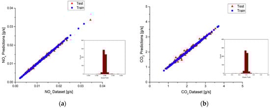
Figure 20.
(a) Deviations between the predictions and the measurements and ground truth plot of the best NOx model in suburbs; (b) Deviations between the predictions and the measurements and ground truth plot of the best CO2 model in suburbs.
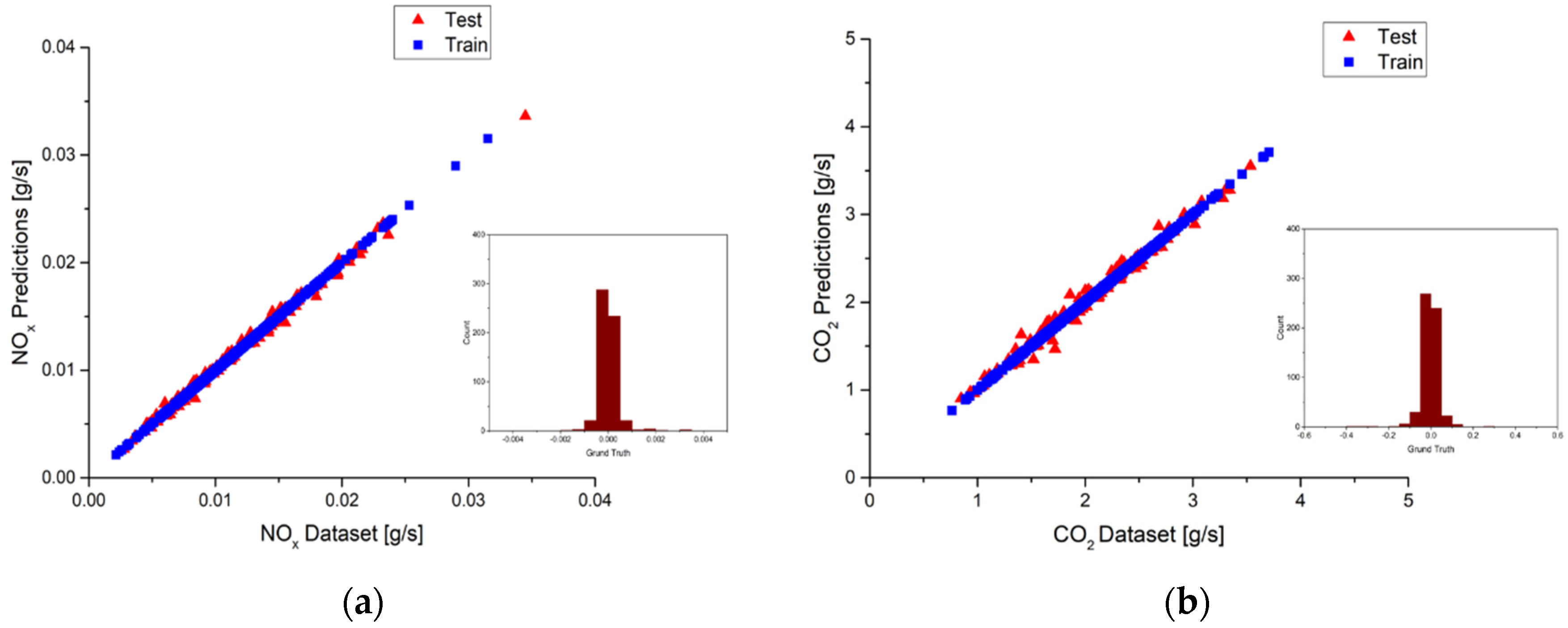
The model performance in the highways part is examined in the following. The best model is built by using the top four features for NOx, and the top nine features are used for the CO2 model according to the results listed in Table 9 and Table 10, respectively. It is noted that the R2 values of both the NOx model and the CO2 model are 0.99. The best NOx and CO2 models prediction results of the test and training sub-datasets are plotted in Figure 21a,b with a red triangle and blue square, respectively. Very few deviations can be observed for the best NOx model in Figure 21a. More deviations can be found for the best CO2 model in Figure 21b because the R2 value is 0.98. The bar charts located in the lower right corner show the ground truth distributions of the predictions. Both models show pretty good accuracy, with the distributions concentrating around zero value.
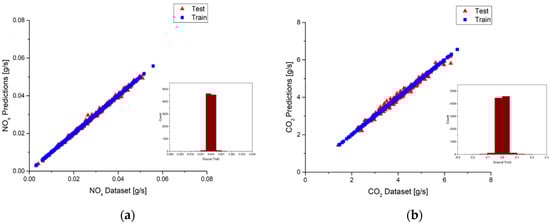
Figure 21.
(a) Deviations between the predictions and the measurements and ground truth plot of the best NOx model in highways; (b) Deviations between the predictions and the measurements and ground truth plot of the best CO2 model in highways.
Figure 22a shows the deviations between the predictions and the measurements by using the top four features as input to build the NOx model in the urban part. Comparisons between Figure 19a and Figure 22a show that the deviations in Figure 22a are a little bit greater than Figure 19a. This is reasonable since the best model has the highest performance R2 value. It is also noted that a similar result as the NOx model is found for the CO2 model in the urban part shown in Figure 22b. Moreover, taking a look at the second route prediction R2 values for the NOx model in the urban route would find that the R2 values of using the top four features for input are close to the R2 value of the best prediction. This is similar to the CO2 model where the R2 values of using the top four features for input is 0.75, and the best prediction has the R2 value of 0.79. As a result, selections of the NOx model and CO2 model that use the top four features could be the second choice for second route prediction.
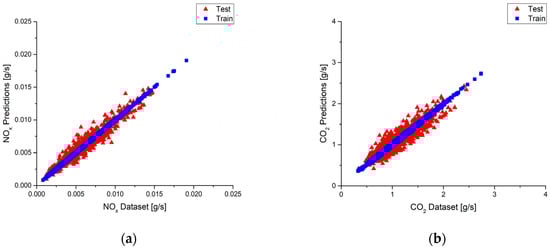
Figure 22.
(a) Deviations between the predictions and the measurements plot of using the top 4 features NOx model in urban. (b) Deviations between the predictions and the measurements plot of using the top 4 features CO2 model in urban.
The purpose of this paper is to find a feasible way to build a predictive model for diesel emissions. It was found that three parameters are good enough to build a model. A lot of computational costs could be saved with the simplified model. The results of this paper would be very useful for the modelers thereafter. The strategy of emission reduction is not the purpose of this paper. However, according to the results of the emission model developed in this paper, the most important features are exhaust flow rate, air–fuel ratio, and engine speed. The implications of the findings are that reducing the engine load may abate the emissions of a running vehicle.
The NOx emission factors calculation from Table 14 shows that the lowest value occurs in the suburbs. It is observed from Table 14 that there is the same trend in the CO2 emission factors calculation. The common reason might be acceleration and deceleration. It would be helpful to remind drivers to control their speed to reduce air pollution.
6. Conclusions
The features importance analysis of NOx and CO2 models for urban, suburb, and highways are built successfully. The top three features of urban, suburban, and highway NOx models are airflow rate, exhaust flow rate, and CO2 concentrations, and the top three features of urban and suburban CO2 models are exhaust flow rate, airflow rate, and engine speed. The top three features of highway CO2 models are airflow rate, exhaust flow rate, and acceleration.
In order to have an accurate prediction, generally, we need more input features. However, the accuracy is not proportional to the number of input features. More input features do not guarantee more accurate predictions. The best models need 4~9 input features to have the highest R2 value. The best predictions of the second route need 4~6 input features. The choice of input features depends on the route characteristics and the emissions.
If the computational cost is a major concern, the model could be simplified to reduce the number of input features. The R2 values of the simplified NOx models using the top three and top four input features are very close to the best model. The difference in R2 values is as small as 0.01. The R2 values of the simplified CO2 models using the top three and top four input features are also very close to the best model. The difference in R2 values is about 0.04.
The purpose of this paper is to find a feasible way to build a predictive model for diesel emissions. It was found that three parameters are good enough to build a model. A lot of computational costs could be saved with the simplified model. The results of this paper would be very useful for the modelers thereafter.
Moreover, the gradient boosting regression model is a very powerful tool in modeling and prediction, and has been applied in many different fields. However, this model has not been used in pollution predictions widely. The NOx and CO2 GBR models were built successfully in this study to predict the emissions of diesel vehicles on real roads with pretty good R2 values. The results show that the GBR is a practical approach to making accurate predictions.
It is recommended that three or four input features are good enough to build an accurate and fast model for the prediction of the NOx and CO2 emissions of diesel vehicles running on real roads. However, the choice of input features is important. An inappropriate choice of input feature may give poor results.
Author Contributions
Conceptualization, H.-T.W. and J.-H.L.; methodology, H.-T.W.; software, H.-T.W.; validation, H.-T.W. and J.-H.L.; data curation, D.-S.J.; writing—original draft preparation, H.-T.W.; writing—review and editing, H.-T.W.; supervision, J.-H.L.; All authors have read and agreed to the published version of the manuscript.
Funding
This research received no external funding.
Institutional Review Board Statement
Not applicable.
Informed Consent Statement
Not applicable.
Data Availability Statement
Data is contained within the article.
Conflicts of Interest
The authors declare no conflict of interest.
References
- WHO Global Urban Ambient Air Pollution Database 2016; World Health Organization: Geneva, Switzerland, 2017.
- Kuo, C.-Y.; Chan, C.-K.; Wu, C.-Y.; Phan, D.-V.; Chan, C.-L. The short-term effects of ambient air pollutants on childhood asthma hospitalization in Taiwan: A national study. Int. J. Environ. Res. Public Health 2019, 16, 203. [Google Scholar] [CrossRef] [PubMed] [Green Version]
- Zhong, S.; Yu, Z.; Zhu, W. Study of the effects of air pollutants on human health based on Baidu indices of disease symptoms and air quality monitoring data in Beijing, China. Int. J. Environ. Res. Public Health 2019, 16, 1014. [Google Scholar] [CrossRef] [Green Version]
- Wang, S.-Y.; Cheng, Y.-Y.; Guo, H.-R.; Tseng, Y.-C. Air Pollution during Pregnancy and Childhood Autism Spectrum Disorder in Taiwan. Int. J. Environ. Res. Public Health 2021, 18, 9784. [Google Scholar] [CrossRef]
- Breuer, J.L.; Samsun, R.C.; Peters, R.; Stolten, D. The impact of diesel vehicles on NOx and PM10 emissions from road transport in urban morphological zones: A case study in North Rhine-Westphalia, Germany. Sci. Total Environ. 2020, 727, 138583. [Google Scholar] [CrossRef]
- Emissions Standards. Available online: https://www.dieselnet.com/standards/eu/ld.php (accessed on 15 June 2021).
- International Transport Forum. 2006. Available online: https://www.itf-oecd.org/sites/default/files/docs/06NOx.pdf (accessed on 15 June 2021).
- Franco, V.; Sanchez, F.P.; German, J.; Mock, P. Real-world exhaust emissions from modern diesel cars. Commun. Int. Counc. Clean Transp. 2014, 49, 847129-102. [Google Scholar]
- Myers, J.; Kelly, T.; Dindal, A.; Willenberg, Z.; Riggs, K. Environmental Technology Verification Report: Clean Air Technologies International, Inc. REMOTE On-Board Emissions Monitor; Battelle: Columbus, OH, USA, 2003. [Google Scholar]
- Jhang, D.-S. Real Road Emission Measurement and Analysis with PEMS for Light Diesel Vehicles; National Chung Hsing University: Taichung, Taiwan, 2018. [Google Scholar]
- Frey, H.C.; Unal, A.; Rouphail, N.M.; Colyar, J.D. On-road measurement of vehicle tailpipe emissions using a portable instrument. J. Air Waste Manag. Assoc. 2003, 53, 992–1002. [Google Scholar] [CrossRef] [PubMed] [Green Version]
- Frey, H.; Zhang, K.; Rouphail, N. Fuel use and emissions comparisons for alternative routes, vehicles, road grade and time of day using in-use measurements. Environ. Sci. Technol. 2008, 42, 2483–8249. [Google Scholar] [CrossRef] [PubMed]
- McCaffery, C.; Zhu, H.; Tang, T.; Li, C.; Karavalakis, G.; Cao, S.; Oshinuga, A.; Burnette, A.; Johnson, K.C.; Durbin, T.D. Real-world NOx emissions from heavy-duty diesel, natural gas, and diesel hybrid electric vehicles of different vocations on California roadways. Sci. Total Environ. 2021, 784, 147224. [Google Scholar] [CrossRef]
- Jaworski, A.; Mądziel, M.; Lejda, K. Creating an emission model based on portable emission measurement system for the purpose of a roundabout. Environ. Sci. Pollut. Res. 2019, 26, 21641–21654. [Google Scholar] [CrossRef] [PubMed] [Green Version]
- Donateo, T.; Filomena, R. Real Time Estimation of Emissions in a Diesel Vehicle with Neural Networks. In Proceedings of the E3S Web of Conferences, EDP Sciences, Ulis, France, September 2020; Volume 197, p. 06020. [Google Scholar]
- Zeng, W.; Miwa, T.; Morikawa, T. Exploring trip fuel consumption by machine learning from GPS and CAN bus data. J. East. Asia Soc. Transp. Stud. 2015, 11, 906–921. [Google Scholar]
- Almér, H. Machine learning and statistical analysis in fuel consumption prediction for heavy vehicles. Engineering 2015. [Google Scholar]
- Thibault, L.; Degeilh, P.; Lepreux, O.; Voise, L.; Alix, G.; Corde, G. A new GPS-based method to estimate real driving emissions. In Proceedings of the 2016 IEEE 19th International Conference on Intelligent Transportation Systems (ITSC), Rio de Janeiro, Brazil, 1–4 November 2016; pp. 1628–1633. [Google Scholar]
- Thibault, L.; Pognant-Gros, P.; Degeilh, P.; Thanabalasingam, K.; Sabiron, G.; Voise, L. Real-time air pollution exposure and vehicle emissions estimation using IoT, GNSS measurements and web-based simulation models. In Proceedings of the 2018 IEEE 88th Vehicular Technology Conference (VTC-Fall), Chicago, IL, USA, 27–30 August 2018; pp. 1–5. [Google Scholar]
- Alimissis, A.; Philippopoulos, K.; Tzanis, C.; Deligiorgi, D. Spatial estimation of urban air pollution with the use of artificial neural network models. Atmos. Environ. 2018, 191, 205–213. [Google Scholar] [CrossRef]
- Bandyopadhyay, G.; Chattopadhyay, S. Single hidden layer artificial neural network models versus multiple linear regression model in forecasting the time series of total ozone. Int. J. Environ. Sci. Technol. 2007, 4, 141–149. [Google Scholar] [CrossRef] [Green Version]
- Gardner, M.; Dorling, S. Neural network modelling and prediction of hourly NOx and NO2 concentrations in urban air in London. Atmos. Environ. 1999, 33, 709–719. [Google Scholar] [CrossRef]
- Perrotta, F.; Parry, T.; Neves, L.C. Application of machine learning for fuel consumption modelling of trucks. In Proceedings of the 2017 IEEE International Conference on Big Data (Big Data), Boston, MA, USA, 11–14 December 2017; pp. 3810–3815. [Google Scholar]
- Zhang, Y.; Haghani, A. A gradient boosting method to improve travel time prediction. Transp. Res. Part C Emerg. Technol. 2015, 58, 308–324. [Google Scholar] [CrossRef]
- Cai, J.; Xu, K.; Zhu, Y.; Hu, F.; Li, L. Prediction and analysis of net ecosystem carbon exchange based on gradient boosting regression and random forest. Appl. Energy 2020, 262, 114566. [Google Scholar] [CrossRef]
- Yang, F.; Wang, D.; Xu, F.; Huang, Z.; Tsui, K.-L. Lifespan prediction of lithium-ion batteries based on various extracted features and gradient boosting regression tree model. J. Power Sources 2020, 476, 228654. [Google Scholar] [CrossRef]
- Wang, T.; Hu, S.; Jiang, Y. Predicting shared-car use and examining nonlinear effects using gradient boosting regression trees. Int. J. Sustain. Transp. 2021, 15, 893–907. [Google Scholar] [CrossRef]
- Wen, H.-T.; Lu, J.-H.; Phuc, M.-X. Applying Artificial Intelligence to Predict the Composition of Syngas Using Rice Husks: A Comparison of Artificial Neural Networks and Gradient Boosting Regression. Energies 2021, 14, 2932. [Google Scholar] [CrossRef]
- Bai, L.; Wang, J.; Ma, X.; Lu, H. Air pollution forecasts: An overview. Int. J. Environ. Res. Public Health 2018, 15, 780. [Google Scholar] [CrossRef] [Green Version]
- Wen, H.-T.; Li, M.-A.; Lu, J.-H. The regression model of NOx emission in a real driving automobile. In Proceedings of the 2019 International Symposium on Intelligent Signal Processing and Communication Systems (ISPACS), Taipei, Taiwan, 3–6 December 2019; pp. 1–2. [Google Scholar]
- Seo, J.; Yun, B.; Park, J.; Park, J.; Shin, M.; Park, S. Prediction of instantaneous real-world emissions from diesel light-duty vehicles based on an integrated artificial neural network and vehicle dynamics model. Sci. Total Environ. 2021, 786, 147359. [Google Scholar] [CrossRef]
- HORIBA. On Board Emission Measurement System OBS-2200-Instruction Manual; HORIBA Ltd.: Kyoto, Japan, 2009. [Google Scholar]
- Zbarcea, O.; Scarpete, D.; Vrabie, V. Environmental Pollution by Diesel Engines. Part II: A Literature Review Regarding Hc, Co, Co2 and Soot Emissions. Termotehnica 2016, 65–69. [Google Scholar]
- Li, C. A Gentle Introduction to Gradient Boosting. 2016. Available online: https://www.ccs.neu.edu/home/vip/teach/MLcourse/4_boosting/slides/gradient_boosting.pdf (accessed on 15 June 2021).
- Friedman, J.H. Greedy function approximation: A gradient boosting machine. Ann. Stat. 2001, 29, 1189–1232. [Google Scholar] [CrossRef]
- John, G.H.; Kohavi, R.; Pfleger, K. Irrelevant features and the subset selection problem. In Machine Learning Proceedings 1994; Elsevier: Amsterdam, The Netherlands, 1994; pp. 121–129. [Google Scholar]
- Casimir, R.; Boutleux, E.; Clerc, G.; Yahoui, A. The use of features selection and nearest neighbors rule for faults diagnostic in induction motors. Eng. Appl. Artif. Intell. 2006, 19, 169–177. [Google Scholar] [CrossRef]
- Dewi, C.; Chen, R.-C. Random forest and support vector machine on features selection for regression analysis. Int. J. Innov. Comput. Inf. Control 2019, 15, 2027–2037. [Google Scholar]


Publisher’s Note: MDPI stays neutral with regard to jurisdictional claims in published maps and institutional affiliations. |
© 2021 by the authors. Licensee MDPI, Basel, Switzerland. This article is an open access article distributed under the terms and conditions of the Creative Commons Attribution (CC BY) license (https://creativecommons.org/licenses/by/4.0/).