
Inter- and Intra-Individual Variability of Personal Health Risk of Combined Particle and Gaseous Pollutants across Selected Urban Microenvironments


Abstract
:1. Introduction
2. Materials and Methods
2.1. Study Design
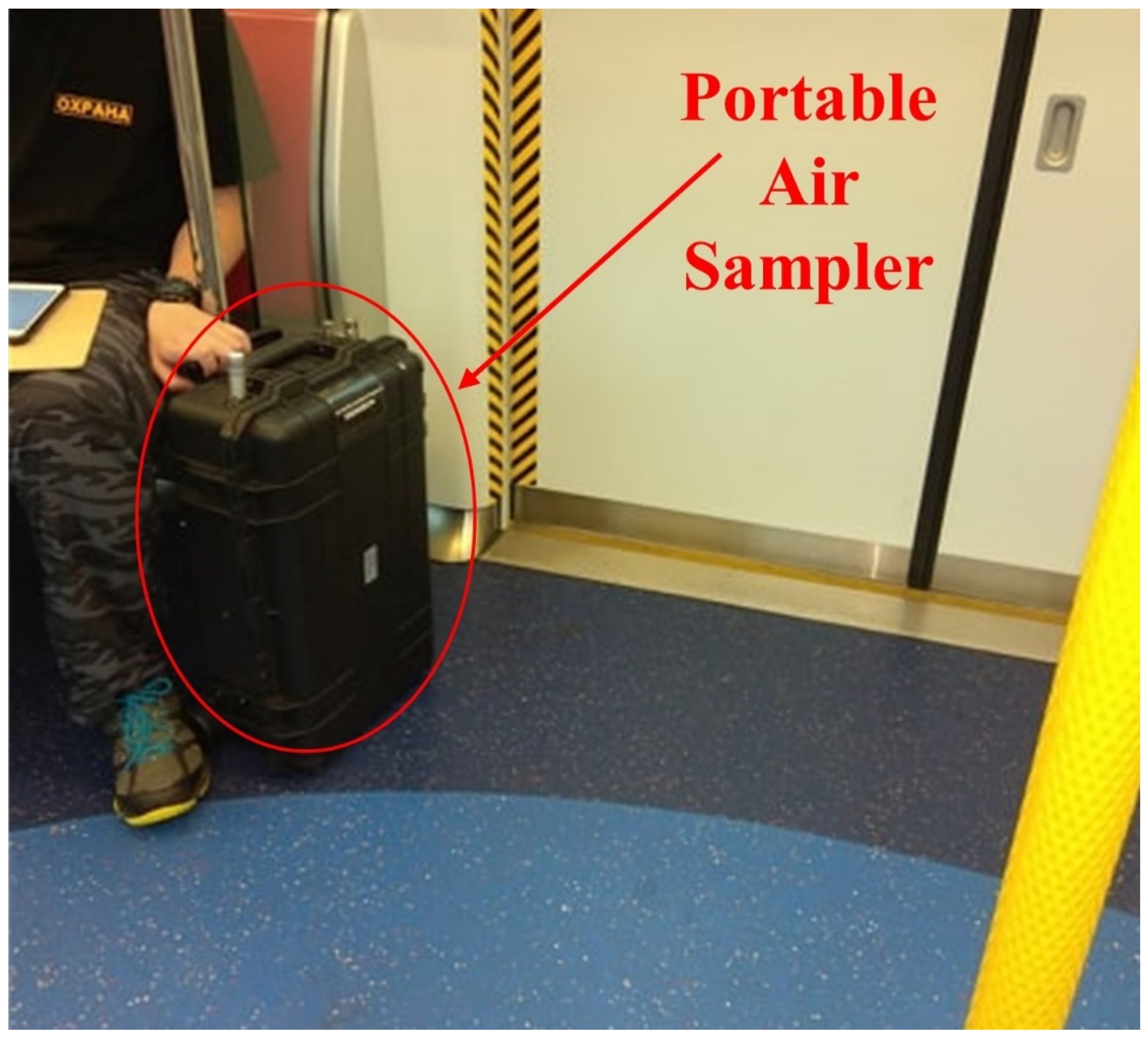
2.2. Instrumentation
2.3. Time-Location Records
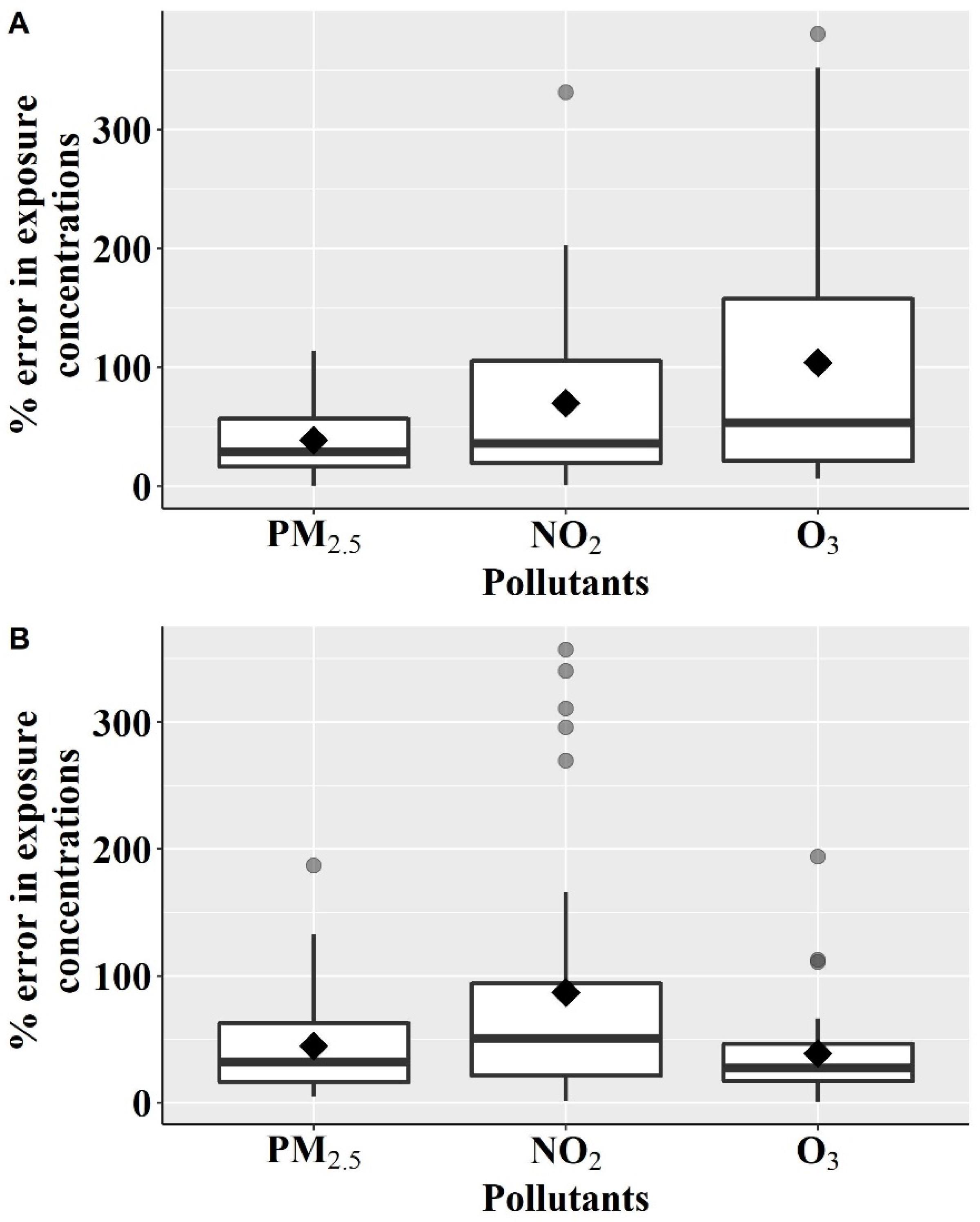
2.4. Quantification of Exposure Error between Personal Exposure Concentrations and Ambient Concentrations
2.5. Calculation of Health Risk
2.6. Time-Integrated Health Risk
2.7. Quantifying Inter- and Intra-Individual Variability in Time-Integrated Health Risk
2.8. Statistical Analysis
3. Results
3.1. Study Participants and Time-Location Pattern
3.2. Exposure Error between Personal Exposure Concentrations and Ambient Concentration
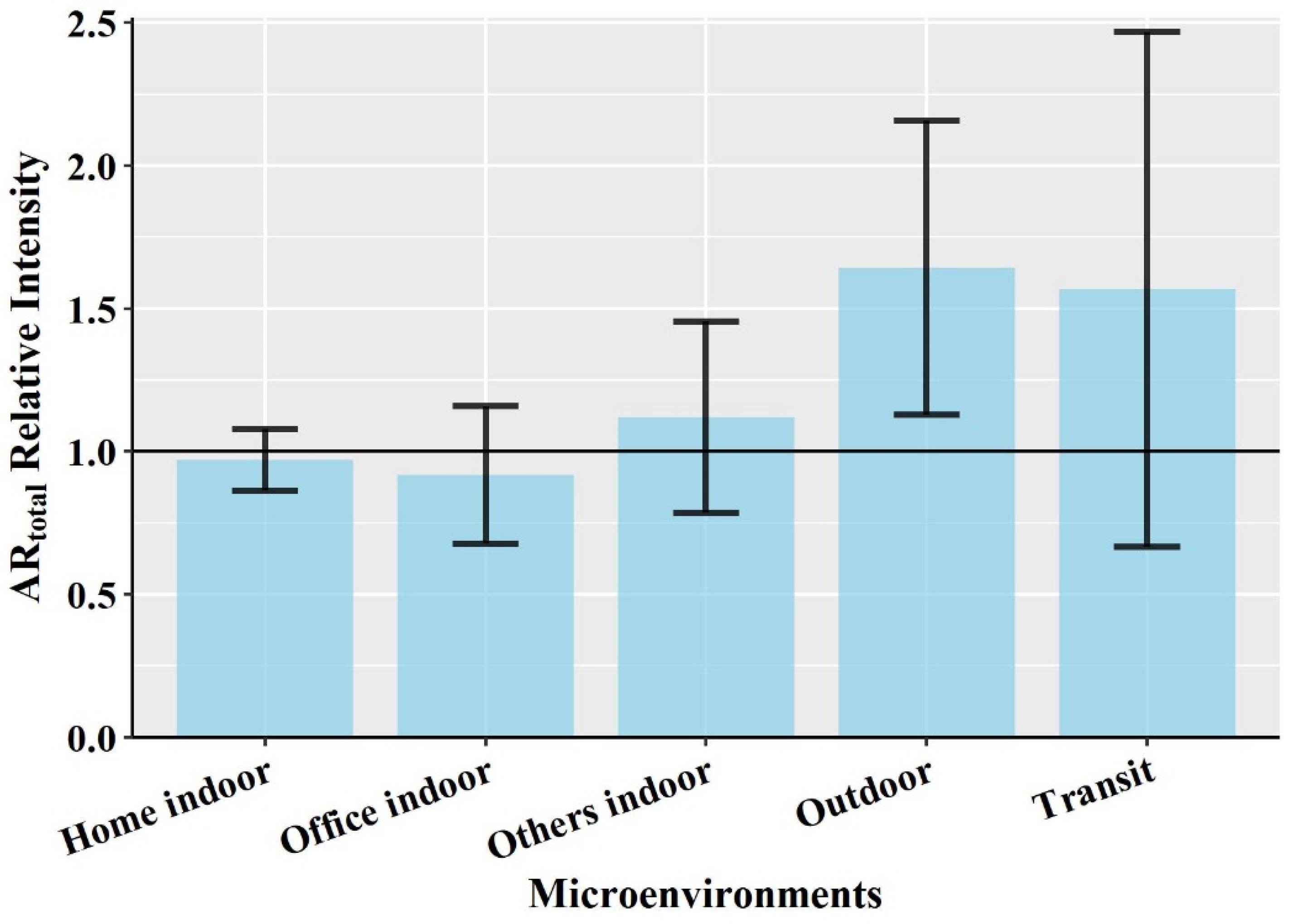
3.3. Contribution of the Selected Microenvironments in Time-Integrated Health Risk
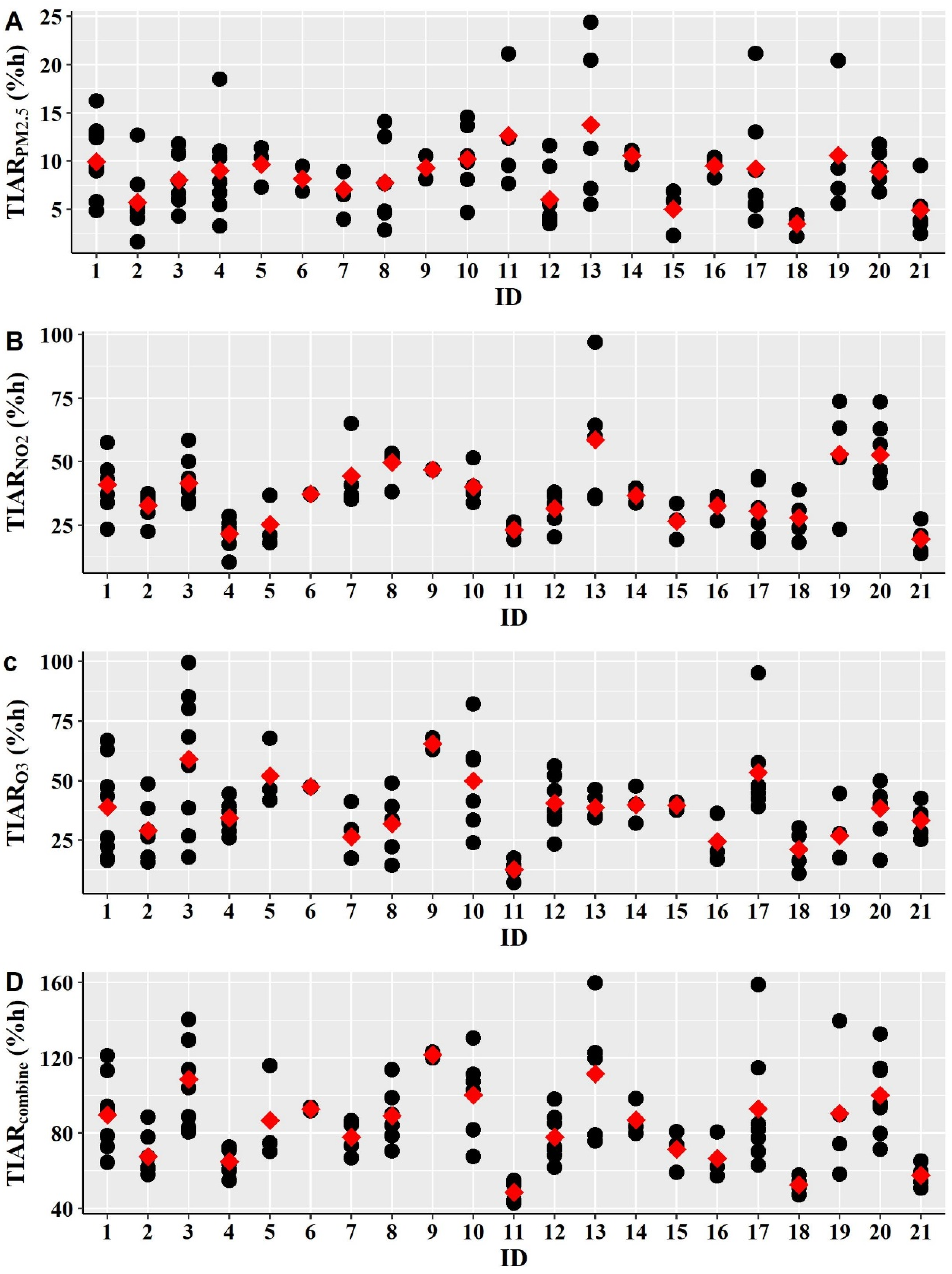
3.4. Inter-Individual and Intra-Individual Variability in Time-Integrated Health Risk
4. Discussion
5. Conclusions
Supplementary Materials
Author Contributions
Funding
Institutional Review Board Statement
Informed Consent Statement
Data Availability Statement
Acknowledgments
Conflicts of Interest
References
- WHO. WHO Global Urban Ambient Air Pollution Database (Update 2016), World Health Organization. 2016. Available online: https://www.who.int/airpollution/data/cities-2016/en/ (accessed on 2 April 2021).
- USEPA. Integrated Science Assessment for Particulate Matter; Center for Public Health and Environmental Assessment, Office of Research and Development, United States Environmental Protection Agency: Research Triangle Park, NC, USA, 2019.
- USEPA. Integrated Science Assessment for Oxides of Nitrogen-Health Criteria; National Center for Environmental Assessment-RTP Division, Office of Research and Development, United States Environmental Protection Agency: Research Triangle Park, NC, USA, 2016.
- USEPA. Integrated Science Assessment for Ozone and Related Photochemical Oxidants (External Review Draft); National Center for Environmental Assessment-RTP Division, Office of Research and Development, United States Environmental Protection Agency: Research Triangle, NC, USA, 2019.
- Li, S.; Batterman, S.; Wasilevich, E.; Wahl, R.; Wirth, J.; Su, F.-C.; Mukherjee, B. Association of daily asthma emergency department visits and hospital admissions with ambient air pollutants among the pediatric Medicaid population in Detroit: Time-series and time-stratified case-crossover analyses with threshold effects. Environ. Res. 2011, 111, 1137–1147. [Google Scholar] [CrossRef]
- Dauchet, L.; Hulo, S.; Cherot-Kornobis, N.; Matran, R.; Amouyel, P.; Edmé, J.-L.; Giovannelli, J. Short-term exposure to air pollution: Associations with lung function and inflammatory markers in non-smoking, healthy adults. Environ. Int. 2018, 121, 610–619. [Google Scholar] [CrossRef] [PubMed]
- Myung, W.; Lee, H.; Kim, H. Short-term air pollution exposure and emergency department visits for amyotrophic lateral sclerosis: A time-stratified case-crossover analysis. Environ. Int. 2019, 123, 467–475. [Google Scholar] [CrossRef]
- Tam, W.W.S.; Wong, T.W.; Wong, A.H. Association between air pollution and daily mortality and hospital admission due to ischaemic heart diseases in Hong Kong. Atmos. Environ. 2015, 120, 360–368. [Google Scholar] [CrossRef]
- Tam, W.W.S.; Wong, T.W.; Ng, L.; Wong, S.Y.-S.; Kung, K.K.L.; Wong, A.H.S. Association between Air Pollution and General Outpatient Clinic Consultations for Upper Respiratory Tract Infections in Hong Kong. PLoS ONE 2014, 9, e86913. [Google Scholar] [CrossRef] [Green Version]
- Habre, R.; Coull, B.; Moshier, E.; Godbold, J.; Grunin, A.; Nath, A.; Castro, W.; Schachter, N.; Rohr, A.; Kattan, M.; et al. Sources of indoor air pollution in New York City residences of asthmatic children. J. Expo. Sci. Environ. Epidemiol. 2014, 24, 269–278. [Google Scholar] [CrossRef]
- Che, W.; Frey, H.C.; Li, Z.; Lao, X.; Lau, A.K.H. Indoor Exposure to Ambient Particles and Its Estimation Using Fixed Site Monitors. Environ. Sci. Technol. 2018, 53, 808–819. [Google Scholar] [CrossRef] [PubMed]
- Hoek, G.; Beelen, R.; De Hoogh, K.; Vienneau, D.; Gulliver, J.; Fischer, P.; Briggs, D. A review of land-use regression models to assess spatial variation of outdoor air pollution. Atmos. Environ. 2008, 42, 7561–7578. [Google Scholar] [CrossRef]
- Eeftens, M.; Beelen, R.; de Hoogh, K.; Bellander, T.; Cesaroni, G.; Cirach, M.; Declercq, C.; Dėdelė, A.; Dons, E.; de Nazelle, A.; et al. Development of Land Use Regression Models for PM2.5, PM2.5 Absorbance, PM10 and PM coarse in 20 european study areas; results of the ESCAPE project. Environ. Sci. Technol. 2012, 46, 11195–11205. [Google Scholar] [CrossRef]
- Zhang, J.J.; Sun, L.; Barrett, O.; Bertazzon, S.; Underwood, F.E.; Johnson, M. Development of land-use regression models for metals associated with airborne particulate matter in a North American city. Atmos. Environ. 2015, 106, 165–177. [Google Scholar] [CrossRef]
- Chen, L.; Bai, Z.; Kong, S.; Han, B.; You, Y.; Ding, X.; Du, S.; Liu, A. A land use regression for predicting NO2 and PM10 concentrations in different seasons in Tianjin region, China. J. Environ. Sci. 2010, 22, 1364–1373. [Google Scholar] [CrossRef]
- Mazaheri, M.; Clifford, S.; Yeganeh, B.; Viana, M.; Rizza, V.; Flament, R.; Buonanno, G.; Morawska, L. Investigations into factors affecting personal exposure to particles in urban microenvironments using low-cost sensors. Environ. Int. 2018, 120, 496–504. [Google Scholar] [CrossRef] [PubMed]
- Koehler, K.; Good, N.; Wilson, A.; Mölter, A.; Moore, B.F.; Carpenter, T.; Peel, J.L.; Volckens, J. The Fort Collins commuter study: Variability in personal exposure to air pollutants by microenvironment. Indoor Air 2019, 29, 231–241. [Google Scholar] [CrossRef] [Green Version]
- Ma, J.; Tao, Y.; Kwan, M.-P.; Chai, Y. Assessing Mobility-Based Real-Time Air Pollution Exposure in Space and Time Using Smart Sensors and GPS Trajectories in Beijing. Ann. Am. Assoc. Geogr. 2020, 110, 434–448. [Google Scholar] [CrossRef]
- Watson, A.Y.; Bates, R.R.; Kennedy, D. Assessment of Human Exposure to Air Pollution: Methods, Measurements, and Models. 1988. Available online: https://www.ncbi.nlm.nih.gov/books/NBK218147/ (accessed on 20 June 2021).
- Van Ryswyk, K.; Wheeler, A.J.; Wallace, L.; Kearney, J.; You, H.; Kulka, R.; Xu, X. Impact of microenvironments and personal activities on personal PM2.5 exposures among asthmatic children. J. Expo. Sci. Environ. Epidemiol. 2014, 24, 260–268. [Google Scholar] [CrossRef] [Green Version]
- Kolluru, S.S.R.; Patra, A.K.; Sahu, S.P. A comparison of personal exposure to air pollutants in different travel modes on national highways in India. Sci. Total Environ. 2018, 619–620, 155–164. [Google Scholar] [CrossRef]
- Yang, F.; Lau, C.F.; Tong, V.W.T.; Zhang, K.K.; Westerdahl, D.; Ng, S.; Ning, Z. Assessment of personal integrated exposure to fine particulate matter of urban residents in Hong Kong. J. Air Waste Manag. Assoc. 2018, 69, 47–57. [Google Scholar] [CrossRef]
- Jahn, H.J.; Kraemer, A.; Chen, X.-C.; Chan, C.-Y.; Engling, G.; Ward, T.J. Ambient and personal PM2.5 exposure assessment in the Chinese megacity of Guangzhou. Atmos. Environ. 2013, 74, 402–411. [Google Scholar] [CrossRef]
- Tunno, B.J.; Dalton, R.; Michanowicz, D.R.; Shmool, J.L.C.; Kinnee, E.; Tripathy, S.; Cambal, L.; Clougherty, J.E. Spatial patterning in PM2.5 constituents under an inversion-focused sampling design across an urban area of complex terrain. Expo. Sci. Environ. Epidemiol. 2016, 26, 385–396. [Google Scholar] [CrossRef] [PubMed] [Green Version]
- Li, N.; Xu, C.; Liu, Z.; Li, N.; Chartier, R.; Chang, J.; Wang, Q.; Wu, Y.; Li, Y.; Xu, D. Determinants of personal exposure to fine particulate matter in the retired adults—Results of a panel study in two megacities, China. Environ. Pollut. 2020, 265, 114989. [Google Scholar] [CrossRef] [PubMed]
- Chen, X.-C.; Jahn, H.J.; Ward, T.J.; Ho, H.C.; Luo, M.; Engling, G.; Kraemer, A. Characteristics and determinants of personal exposure to PM2.5 mass and components in adult subjects in the megacity of Guangzhou, China. Atmos. Environ. 2020, 224, 117295. [Google Scholar] [CrossRef]
- Chen, X.-C.; Ward, T.J.; Cao, J.-J.; Lee, S.-C.; Chow, J.C.; Lau, G.N.; Yim, S.H.L.; Ho, K.-F. Determinants of personal exposure to fine particulate matter (PM2.5) in adult subjects in Hong Kong. Sci. Total Environ. 2018, 628–629, 1165–1177. [Google Scholar] [CrossRef] [PubMed]
- Sanchez, M.; Milà, C.; Sreekanth, V.; Balakrishnan, K.; Sambandam, S.; Nieuwenhuijsen, M.; Kinra, S.; Marshall, J.D.; Tonne, C. Personal exposure to particulate matter in peri-urban India: Predictors and association with ambient concentration at residence. J. Expo. Sci. Environ. Epidemiol. 2020, 30, 596–605. [Google Scholar] [CrossRef] [Green Version]
- Lee, K.; Bartell, S.M.; Paek, M. Interpersonal and daily variability of personal exposures to nitrogen dioxide and sulfur dioxide. J. Expo. Sci. Environ. Epidemiol. 2004, 14, 137–143. [Google Scholar] [CrossRef] [Green Version]
- Grivas, G.; Dimakopoulou, K.; Samoli, E.; Papakosta, D.; Karakatsani, A.; Katsouyanni, K.; Chaloulakou, A. Ozone exposure assessment for children in Greece-Results from the RESPOZE study. Sci. Total Environ. 2017, 581–582, 518–529. [Google Scholar] [CrossRef]
- Wong, T.W.; Tam, W.; Yu, I.T.S.; Lau, A.; Pang, S.W.; Wong, A.H. Developing a risk-based air quality health index. Atmos. Environ. 2013, 76, 52–58. [Google Scholar] [CrossRef]
- HKEPD. Air Quality Health Index-Frequently Asked Questions. Environmental Protection Department, Hong Kong, 2019. Available online: http://www.aqhi.gov.hk/en/what-is-aqhi/faqs.html#e_05 (accessed on 14 October 2019).
- Hossain, S.; Frey, H.C.; Louie, P.K.; Lau, A.K. Combined effects of increased O3 and reduced NO2 concentrations on short-term air pollution health risks in Hong Kong. Environ. Pollut. 2021, 270, 116280. [Google Scholar] [CrossRef] [PubMed]
- Lee, S.C.; Cheng, Y.; Ho, K.F.; Cao, J.J.; Louie, P.K.-K.; Chow, J.C.; Watson, J. PM1.0 and PM2.5 characteristics in the roadside environment of Hong Kong. Aerosol Sci. Technol. 2006, 40, 157–165. [Google Scholar] [CrossRef] [Green Version]
- Che, W.; Tso, C.Y.; Sun, L.; Ip, D.Y.; Lee, H.; Chao, Y.H.C.; Lau, A.K. Energy consumption, indoor thermal comfort and air quality in a commercial office with retrofitted heat, ventilation and air conditioning (HVAC) system. Energy Build. 2019, 201, 202–215. [Google Scholar] [CrossRef]
- Sun, L.; Wong, K.C.; Wei, P.; Ye, S.; Huang, H.; Yang, F.; Westerdahl, D.; Louie, P.K.; Luk, C.W.; Ning, Z. Development and application of a next generation air sensor network for the Hong Kong marathon 2015 air quality monitoring. Sensors 2016, 16, 211. [Google Scholar] [CrossRef]
- Sun, L.; Westerdahl, D.; Ning, Z. Development and evaluation of a novel and cost-effective approach for low-cost NO2 sensor drift correction. Sensors 2017, 17, 1916. [Google Scholar] [CrossRef] [PubMed]
- Che, W.; Li, A.T.Y.; Frey, H.C.; Tang, K.T.J.; Sun, L.; Wei, P.; Hossain, S.; Hohenberger, T.L.; Leung, K.W.; Lau, A.K.H. Factors affecting variability in gaseous and particle microenvironmental air pollutant concentrations in Hong Kong primary and secondary schools. Indoor Air 2020, 31, 170–187. [Google Scholar] [CrossRef]
- Hossain, S.; Che, W.; Frey, H.C.; Lau, A.K. Factors affecting variability in infiltration of ambient particle and gaseous pollutants into home at urban environment. Build. Environ. 2021, 206, 108351. [Google Scholar] [CrossRef]
- Persily, A.K. Evaluating building IAQ and ventilation with indoor carbon dioxide. ASHRAE Trans. 1997, 103, 193–204. [Google Scholar]
- Satish, U.; Mendell, M.J.; Shekhar, K.; Hotchi, T.; Sullivan, D.; Streufert, S.; Fisk, W.J. Is CO2 an Indoor Pollutant? Direct Effects of Low-to-Moderate CO2 Concentrations on Human Decision-Making Performance. Environ. Health Perspect. 2012, 120, 1671–1677. [Google Scholar] [CrossRef] [Green Version]
- Klepeis, N.E. An introduction to the indirect exposure assessment approach: Modeling human exposure using microenvironmental measurements and the recent National Human Activity Pattern Survey. Environ. Health Perspect. 1999, 107, 365–374. [Google Scholar] [CrossRef] [PubMed]
- Mazaheri, M.; Clifford, S.; Jayaratne, R.; Mokhtar, M.A.M.; Fuoco, F.; Buonanno, G.; Morawska, L. School children’s personal exposure to ultrafine particles in the urban environment. Environ. Sci. Technol. 2013, 48, 113–120. [Google Scholar] [CrossRef] [PubMed] [Green Version]
- Xu, R. Measuring explained variation in linear mixed effects models. Stat. Med. 2003, 22, 3527–3541. [Google Scholar] [CrossRef]
- Sahai, H.; Ageel, M.I. The Analysis of Variance: Fixed, Random, and Mixed Models; Birkhäuser: Boston, MA, USA, 2000. [Google Scholar]
- Xu, M.; Sbihi, H.; Pan, X.; Brauer, M. Local variation of PM2.5 and NO2 concentrations within metropolitan Beijing. Atmos. Environ. 2019, 200, 254–263. [Google Scholar] [CrossRef]
- Squizzato, S.; Masiol, M.; Rich, D.Q.; Hopke, P.K. PM2.5 and gaseous pollutants in New York State during 2005–2016: Spatial variability, temporal trends, and economic influences. Atmos. Environ. 2018, 183, 209–224. [Google Scholar] [CrossRef]
- Baxter, L.K.; Clougherty, J.E.; Laden, F.; Levy, J.I. Predictors of concentrations of nitrogen dioxide, fine particulate matter, and particle constituents inside of lower socioeconomic status urban homes. J. Expo. Sci. Environ. Epidemiol. 2007, 17, 433–444. [Google Scholar] [CrossRef] [Green Version]
- Schober, P.; Boer, C.; Schwarte, L.A. Correlation coefficients: Appropriate use and interpretation. Anesth. Analg. 2018, 126, 1763–1768. [Google Scholar] [CrossRef]
- Che, W.; Frey, H.C.; Fung, J.C.; Ning, Z.; Qu, H.; Lo, H.K.; Chen, L.; Wong, T.-W.; Wong, M.K.; Lee, O.C.; et al. PRAISE-HK: A personalized real-time air quality informatics system for citizen participation in exposure and health risk management. Sustain. Cities Soc. 2020, 54, 101986. [Google Scholar] [CrossRef]
- IQAir. IQAir | The World’s Leading Air Quality App. 2021. Available online: https://www.iqair.com/air-quality-app (accessed on 4 June 2021).
- BreezoMeter. Accurate Air Quality, Pollen & Active Fires Information|BreezoMeter. 2021. Available online: https://www.breezometer.com/ (accessed on 4 June 2021).
- AirMatters. Air Matters—A Global Air Quality Service Provider. 2021. Available online: https://air-matters.com/index.html (accessed on 4 June 2021).
- USDOS. ZephAir App Available Now—United States Department of State. 2021. Available online: https://www.state.gov/zephair-app-available-now/ (accessed on 4 June 2021).
- PlumeLabs. Plume Labs App: Live and Forecast air Quality Data. 2021. Available online: https://plumelabs.com/en/air/ (accessed on 4 June 2021).
- Allen, R.W.; Adar, S.D.; Avol, E.; Cohen, M.; Curl, C.L.; Larson, T.; Liu, L.-J.S.; Sheppard, L.; Kaufman, J. Modeling the Residential Infiltration of Outdoor PM 2.5 in the Multi-Ethnic Study of Atherosclerosis and Air Pollution (MESA Air). Environ. Health Perspect. 2012, 120, 824–830. [Google Scholar] [CrossRef] [Green Version]
- Zhou, X.; Cai, J.; Zhao, Y.; Chen, R.; Wang, C.; Zhao, A.; Yang, C.; Li, H.; Liu, S.; Cao, J.; et al. Estimation of residential fine particulate matter infiltration in Shanghai, China. Environ. Pollut. 2016, 233, 494–500. [Google Scholar] [CrossRef]
- Xu, C.; Li, N.; Yang, Y.; Li, Y.; Liu, Z.; Wang, Q.; Zheng, T.; Civitarese, A.; Xu, D. Investigation and modeling of the residential infiltration of fine particulate matter in Beijing, China. J. Air Waste Manag. Assoc. 2017, 67, 694–701. [Google Scholar] [CrossRef] [PubMed]
- MacNeill, M.; Wallace, L.; Kearney, J.; Allen, R.; Van Ryswyk, K.; Judek, S.; Xu, X.; Wheeler, A. Factors influencing variability in the infiltration of PM 2.5 mass and its components. Atmos. Environ. 2012, 61, 518–532. [Google Scholar] [CrossRef]
- Dėdelė, A.; Miškinytė, A. Seasonal variation of indoor and outdoor air quality of nitrogen dioxide in homes with gas and electric stoves. Environ. Sci. Pollut. Res. 2016, 23, 17784–17792. [Google Scholar] [CrossRef] [PubMed]
- Dobbin, N.A.; Sun, L.; Wallace, L.; Kulka, R.; You, H.; Shin, T.; Aubin, D.; St-Jean, M.; Singer, B.C. The benefit of kitchen exhaust fan use after cooking—An experimental assessment. Build. Environ. 2018, 135, 286–296. [Google Scholar] [CrossRef]
- Hu, Y.; Zhao, B. Relationship between indoor and outdoor NO2: A review. Build. Environ. 2020, 180, 106909. [Google Scholar] [CrossRef]
- Huang, Y.; Yang, Z.; Gao, Z. Contributions of indoor and outdoor sources to ozone in residential buildings in Nanjing. Int. J. Environ. Res. Public Health 2019, 16, 2587. [Google Scholar] [CrossRef] [PubMed] [Green Version]
- Lee, S.-C.; Lam, S.; Fai, H.K. Characterization of VOCs, ozone, and PM10 emissions from office equipment in an environmental chamber. Build. Environ. 2001, 36, 837–842. [Google Scholar] [CrossRef]
- Britigan, N.; Alshawa, A.; Nizkorodov, S.A. Quantification of ozone levels in indoor environments generated by ionization and ozonolysis air purifiers. J. Air Waste Manag. Assoc. 2006, 56, 601–610. [Google Scholar] [CrossRef] [Green Version]
- Guo, C.; Gao, Z.; Shen, J. Emission rates of indoor ozone emission devices: A literature review. Build. Environ. 2019, 158, 302–318. [Google Scholar] [CrossRef]


| Microenvironment | Min | P25 | Median | Mean | P75 | Max | SD |
|---|---|---|---|---|---|---|---|
| Home indoor | 9.3 | 12.4 | 14.5 | 15.7 | 18.3 | 24.0 | 4.1 |
| Office indoor | 0 | 1.4 | 6.0 | 5.7 | 9.2 | 13.9 | 4.1 |
| Others indoor | 0 | 0.1 | 0.2 | 1.1 | 1.4 | 7.5 | 1.7 |
| Outdoor | 0 | 0.1 | 0.4 | 0.6 | 0.8 | 4.6 | 0.7 |
| Transit | 0 | 0 | 0.7 | 0.9 | 1.5 | 5.8 | 1.0 |
| Pollutants a | ||
|---|---|---|
| TIARPM2.5 | 22 | 78 |
| TIARNO2 | 54 | 46 |
| TIARO3 | 40 | 60 |
| TIARcombine b | 53 | 47 |
| Variables a | Participant Wise Average TIARcombine | Daily TIARcombine | ||
|---|---|---|---|---|
| Correlation Coefficient (r) | p-Value | Correlation Coefficient (r) | p-Value | |
| Time spent at home indoor | −0.09 | 0.70 | 0.20 | 0.04 |
| Time spent at office indoor | 0.14 | 0.54 | −0.02 | 0.84 |
| Time spent at others indoor | −0.36 | 0.12 | −0.07 | 0.54 |
| Time spent at outdoor | 0.05 | 0.84 | 0.17 | 0.13 |
| Time spent at transit | 0.41 | 0.09 | 0.17 | 0.15 |
| PM2.5 (µg/m3) at home indoor | 0.48 | 0.03 | 0.51 | <0.001 |
| PM2.5 (µg/m3) at office indoor | 0.03 | 0.89 | 0.16 | 0.15 |
| PM2.5 (µg/m3) at others indoor | 0.45 | <0.05 | 0.27 | 0.01 |
| PM2.5 (µg/m3) at outdoor | 0.40 | 0.07 | 0.33 | 0.002 |
| PM2.5 (µg/m3) at transit | 0.27 | 0.27 | 0.19 | 0.09 |
| NO2 (µg/m3) at home indoor | 0.60 | 0.004 | 0.56 | <0.001 |
| NO2 (µg/m3) at office indoor | 0.12 | 0.60 | 0.15 | 0.18 |
| NO2 (µg/m3) at others indoor | 0.51 | 0.02 | 0.46 | <0.001 |
| NO2 (µg/m3) at outdoor | 0.24 | 0.30 | 0.33 | 0.002 |
| NO2 (µg/m3) at transit | 0.46 | 0.06 | 0.40 | <0.001 |
| O3 (µg/m3) at home indoor | 0.74 | <0.001 | 0.76 | <0.001 |
| O3 (µg/m3) at office indoor | 0.52 | 0.02 | 0.51 | <0.001 |
| O3 (µg/m3) at others indoor | 0.29 | 0.22 | 0.22 | 0.05 |
| O3 (µg/m3) at outdoor | 0.14 | 0.53 | 0.28 | 0.01 |
| O3 (µg/m3) at transit | −0.08 | 0.76 | −0.06 | 0.61 |
| Ambient PM2.5 (µg/m3) | 0.56 | 0.01 | 0.59 | <0.001 |
| Ambient NO2 (µg/m3) | 0.04 | 0.86 | 0.06 | 0.52 |
| Ambient O3 (µg/m3) | 0.07 | 0.77 | 0.41 | <0.001 |
Publisher’s Note: MDPI stays neutral with regard to jurisdictional claims in published maps and institutional affiliations. |
© 2022 by the authors. Licensee MDPI, Basel, Switzerland. This article is an open access article distributed under the terms and conditions of the Creative Commons Attribution (CC BY) license (https://creativecommons.org/licenses/by/4.0/).
Share and Cite
Hossain, S.; Che, W.; Lau, A.K.-H. Inter- and Intra-Individual Variability of Personal Health Risk of Combined Particle and Gaseous Pollutants across Selected Urban Microenvironments. Int. J. Environ. Res. Public Health 2022, 19, 565. https://doi.org/10.3390/ijerph19010565
Hossain S, Che W, Lau AK-H. Inter- and Intra-Individual Variability of Personal Health Risk of Combined Particle and Gaseous Pollutants across Selected Urban Microenvironments. International Journal of Environmental Research and Public Health. 2022; 19(1):565. https://doi.org/10.3390/ijerph19010565
Chicago/Turabian StyleHossain, Shakhaoat, Wenwei Che, and Alexis Kai-Hon Lau. 2022. "Inter- and Intra-Individual Variability of Personal Health Risk of Combined Particle and Gaseous Pollutants across Selected Urban Microenvironments" International Journal of Environmental Research and Public Health 19, no. 1: 565. https://doi.org/10.3390/ijerph19010565
APA StyleHossain, S., Che, W., & Lau, A. K.-H. (2022). Inter- and Intra-Individual Variability of Personal Health Risk of Combined Particle and Gaseous Pollutants across Selected Urban Microenvironments. International Journal of Environmental Research and Public Health, 19(1), 565. https://doi.org/10.3390/ijerph19010565