
Evaluation of Highway Hydroplaning Risk Based on 3D Laser Scanning and Water-Film Thickness Estimation

 ,
,
Abstract
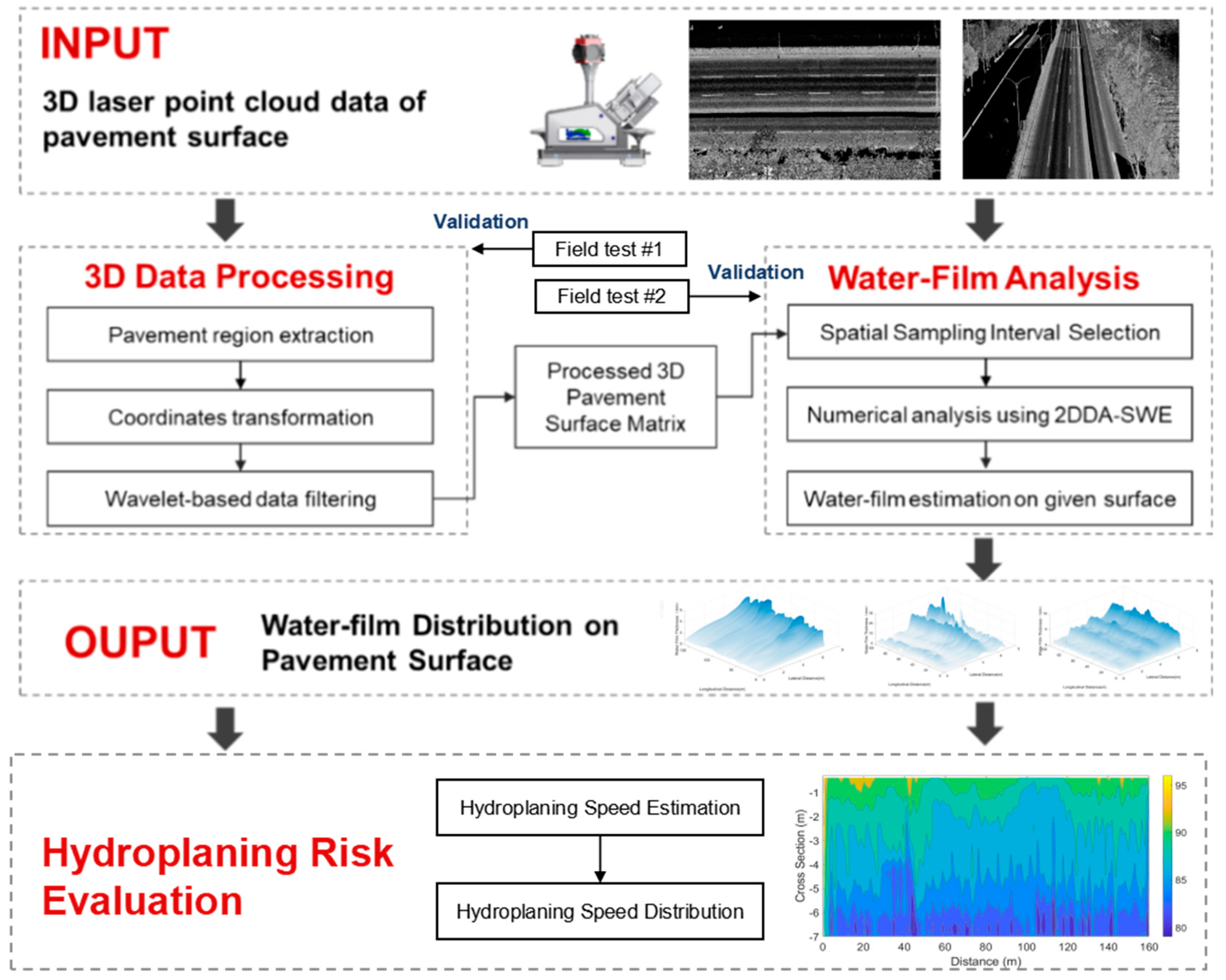
:1. Introduction
2. 3D Laser Scanning Data
2.1. Data Description
2.2. 3D Data Processing
- (1)
- Pavement region extraction (Figure 2).
- (2)
- Coordinates transformation.
| Algorithm 1. Numerical Algorithm for Coordinates Rotation |
| STEP 1. Input the 3D surface data, and extract the plane coordinates x, y. |
| STEP 2. Estimate the slope of the plane coordinates s using linear fitting. |
| STEP 3. Verify the slope condition: |
| (i) if s ≤ 0.05, proceed to Step 6. |
| (ii) if s > 0.05, proceed to Step 4. |
| STEP 4. Calculate θ based on s using the equation: |
| STEP 5. Calculate the rotated matrix using Equation (3). Return to Step 2 and continue the slope calculation until the slope condition is satisfied. |
| STEP 6. Output the final coordinates matrix as the rotated result. |
- (3)
- Point cloud data denoising and filtering.
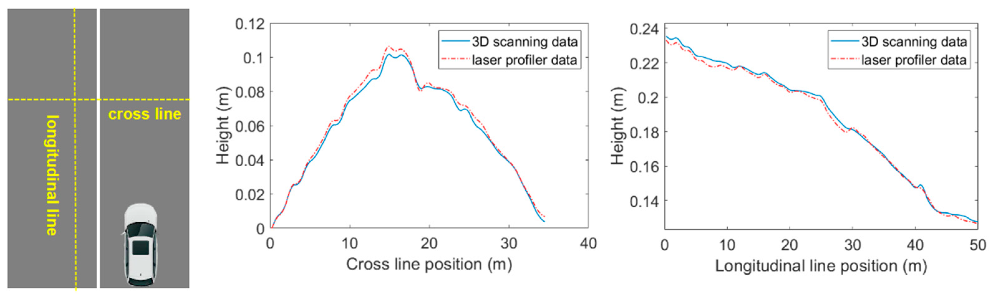
2.3. Validation for 3D Road Surface Measurement
3. Water-Film Prediction Based on 3D Surface Data
3.1. Governing Equations
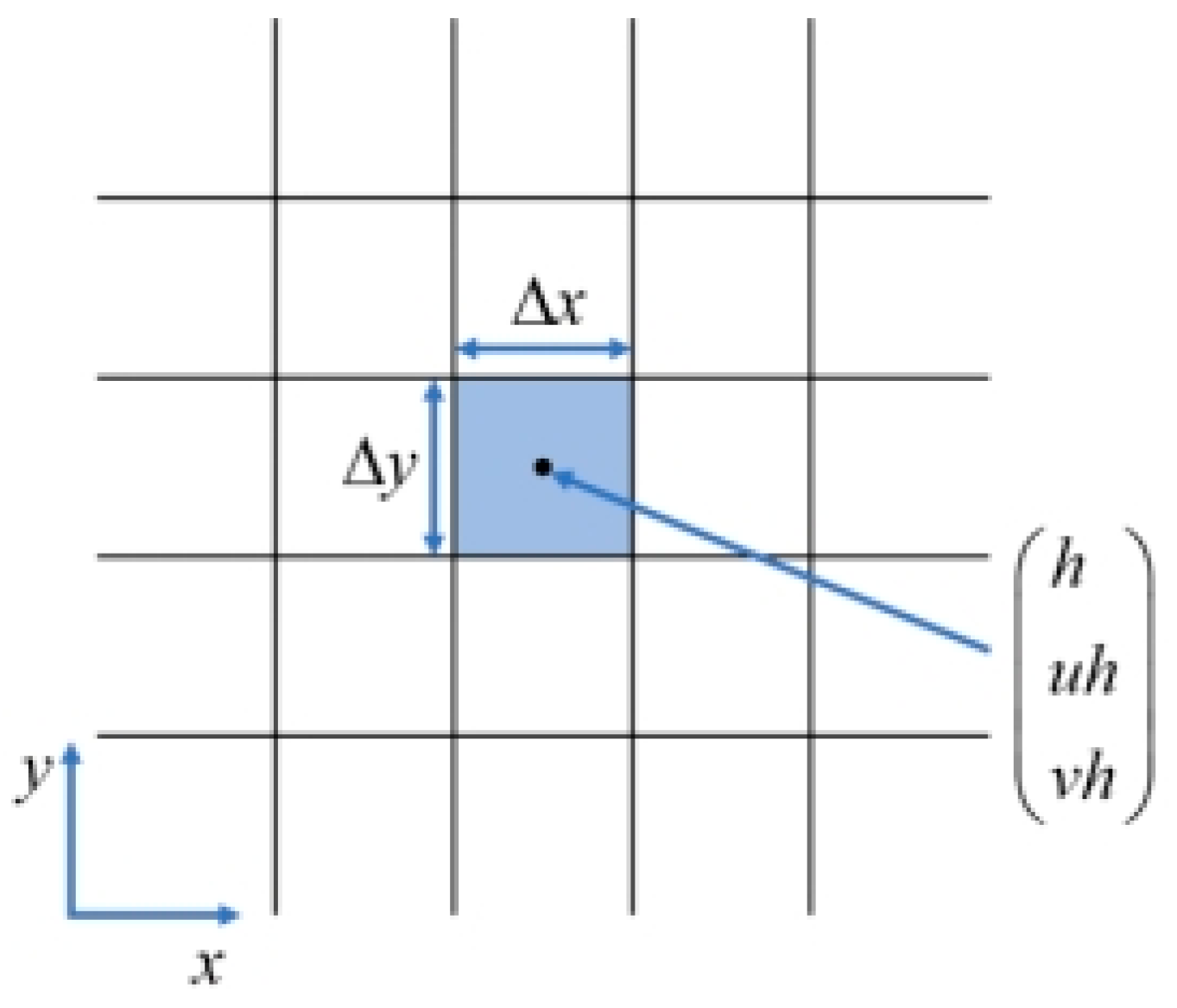
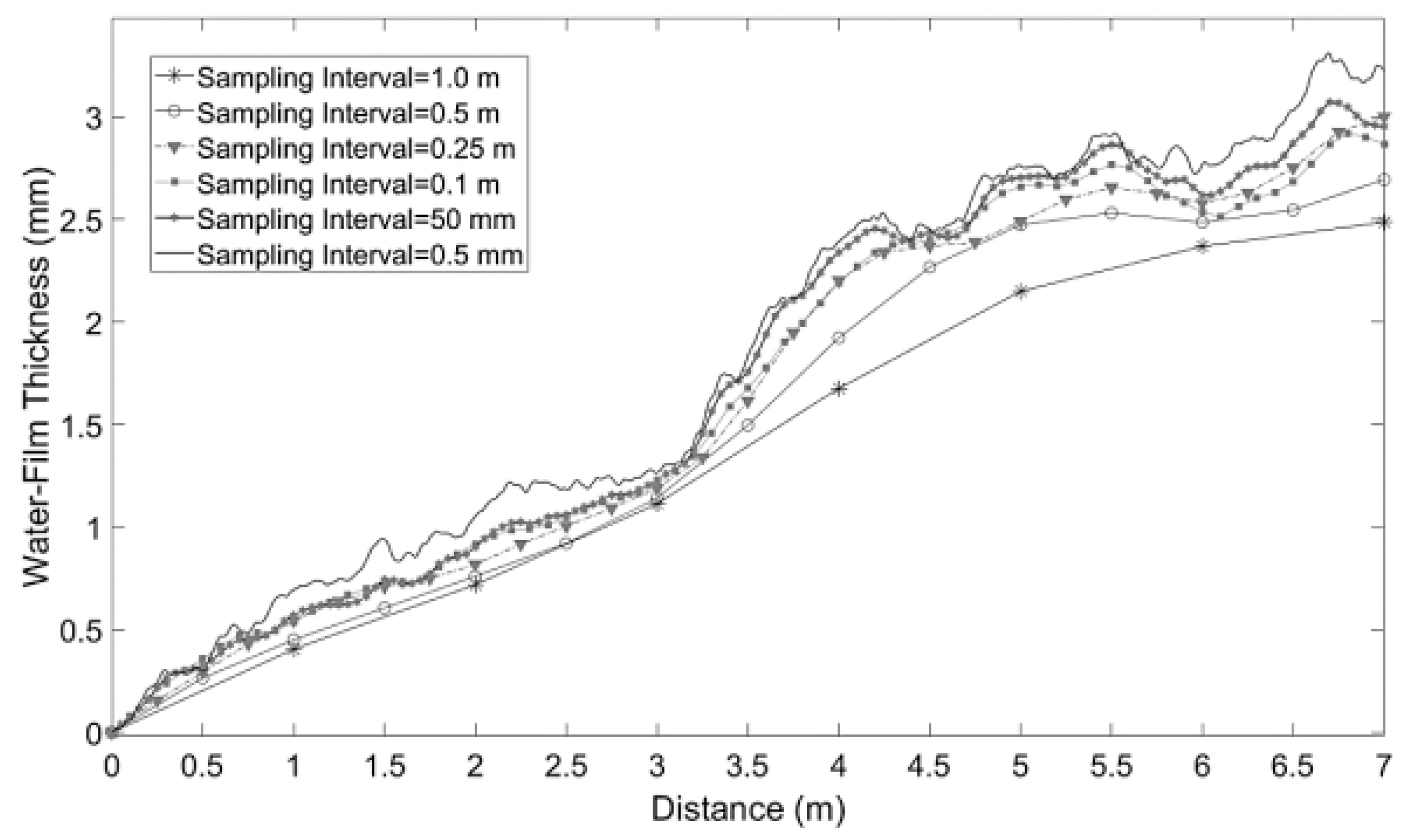
3.2. Numerical Algorithms
| Algorithm 2. Numerical Algorithm for 2DDA-SWE |
| STEP 1. Input 3D surface data, rainfall intensity data, and initial parameters. The values of z, qr, g, and nc are known. Set the calculation period T and initial the model time t = 0. |
| STEP 2. According to solution time and accuracy requirements, set time step Δt and spatial step Δx and Δy. |
| STEP 3. Calculate the intercell flux by Equations (7)–(9). |
| STEP 4. Update the model time to t = (n + 1) Δt by Equation (6). |
| STEP 5. Verify the CFL condition: |
| (i) if CFL ≤ 1, proceed to Step 6. |
| (ii) if CFL > 1, increase Δx and Δy or decrease Δt. Then return to Step 3. |
| STEP 6. Return to Step 3 and continue until the calculation period is completed. |
3.3. Model Parameter Acquisition
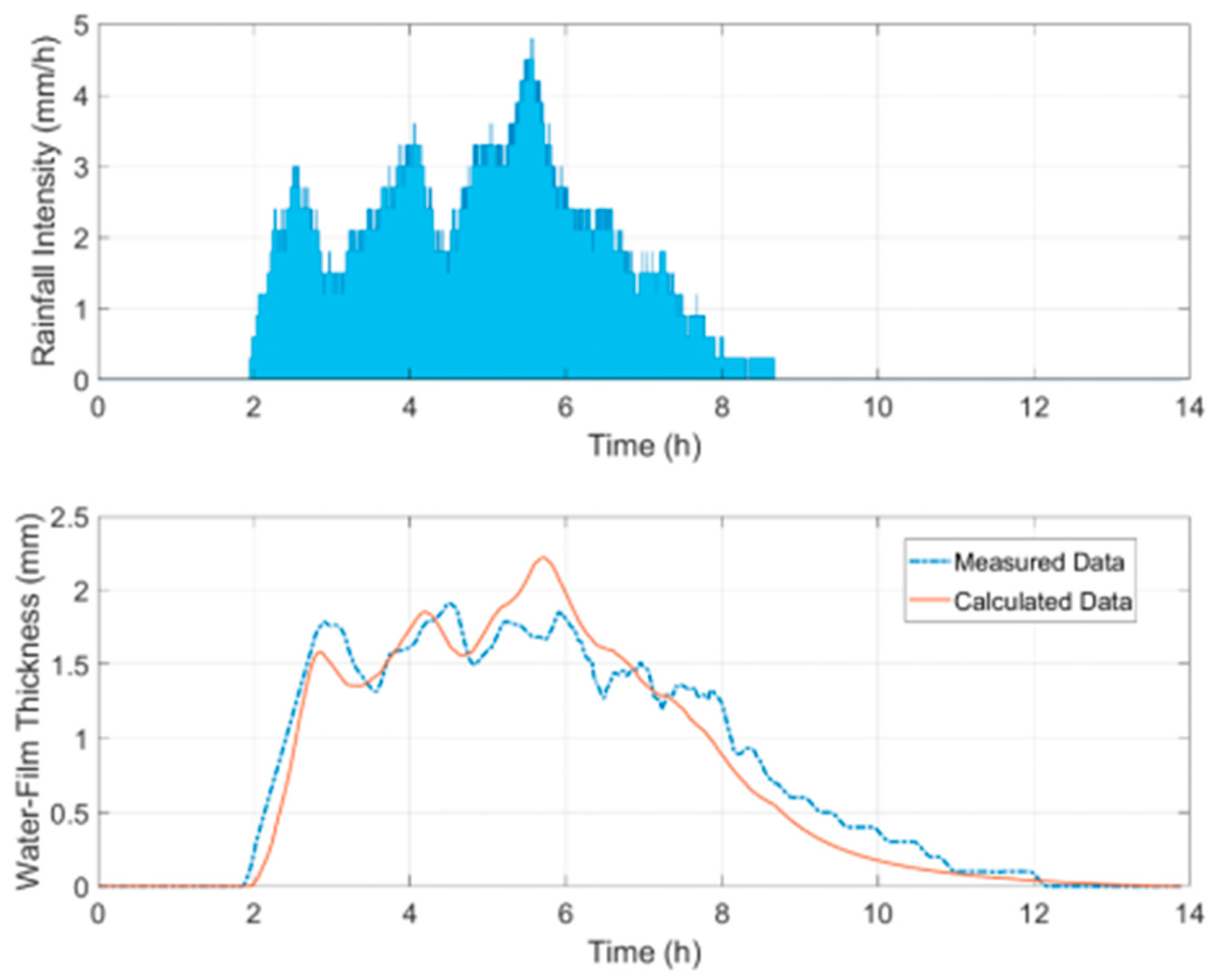
3.4. Model Validation
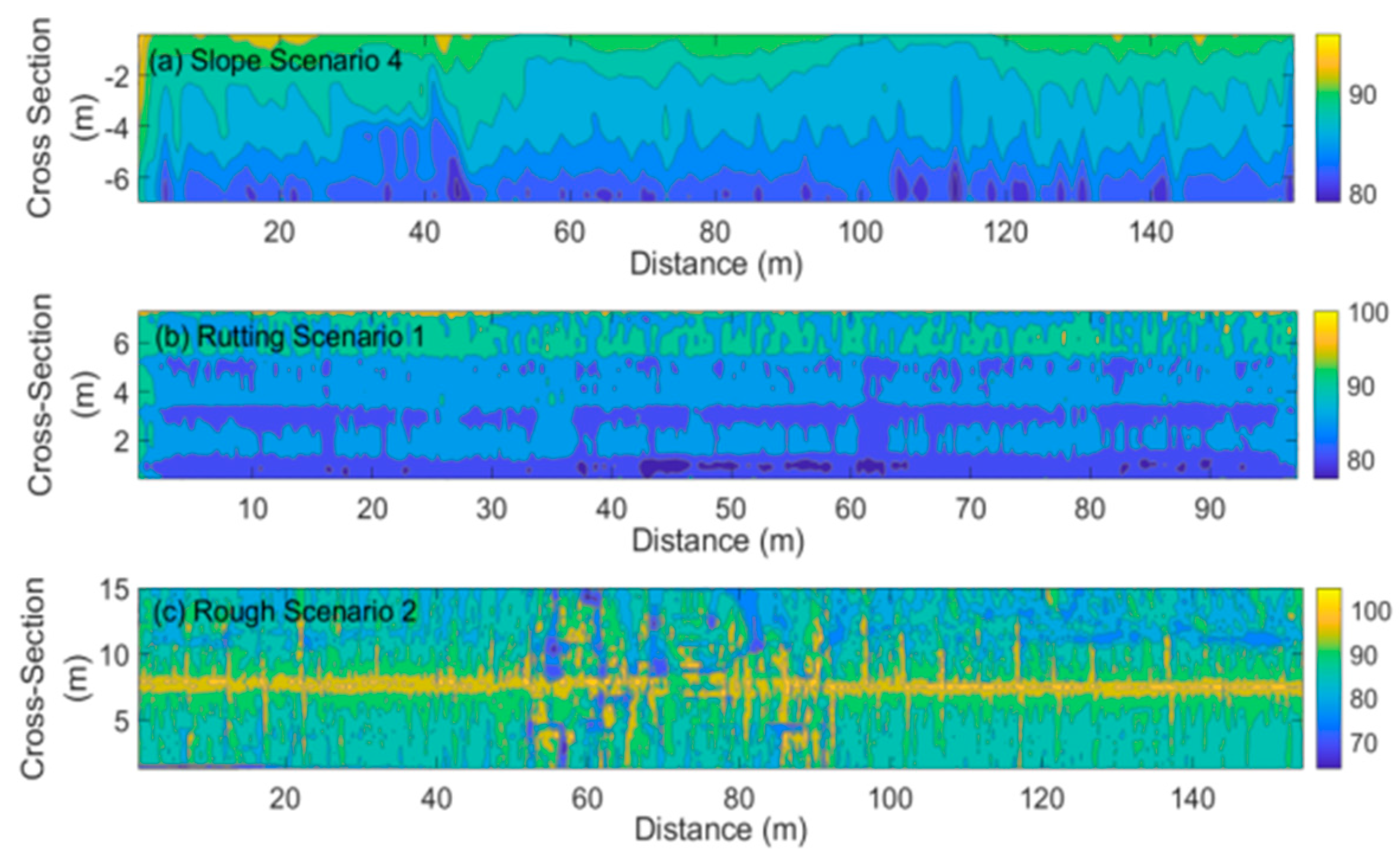
4. Water-Film Thickness Estimation on Road Surfaces with Different Profiles
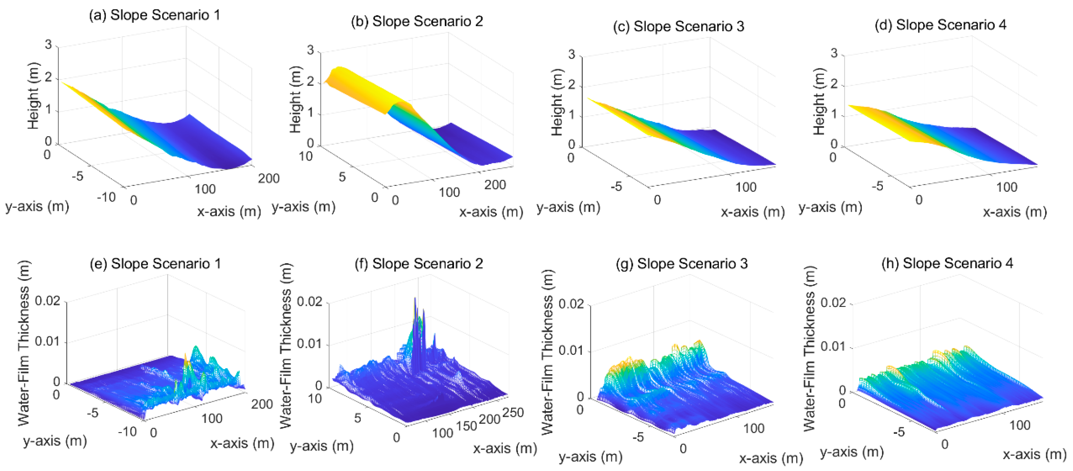
4.1. Surface with Slope
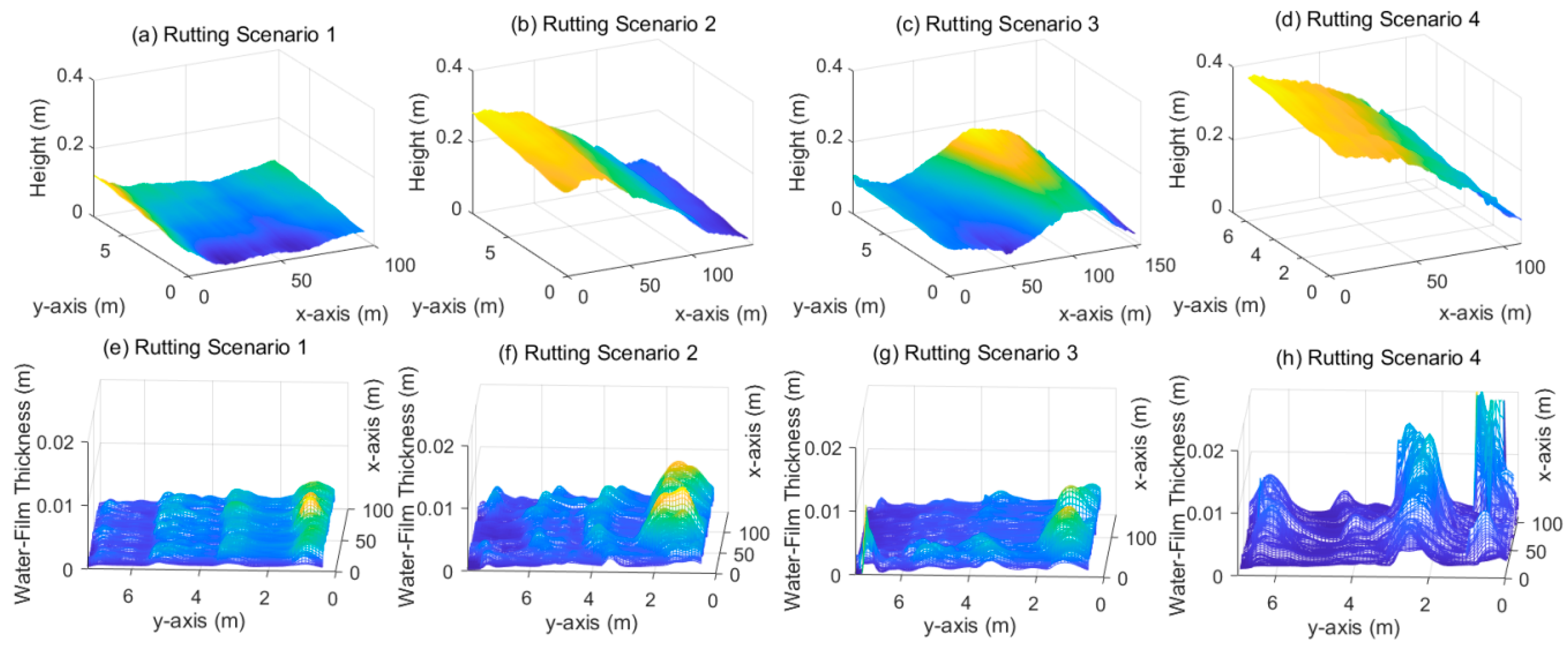
4.2. Surface with Rutting
4.3. Rough Surface
5. Hydroplaning Risk Evaluation
6. Conclusions
Author Contributions
Funding
Institutional Review Board Statement
Informed Consent Statement
Data Availability Statement
Conflicts of Interest
References
- Ding, Y.; Li, D.; Huang, M.; Cao, X.; Tang, B. Study on the Influence of Skid Resistance on Traffic Safety of Highway with a High Ratio of Bridges and Tunnels. Transp. Saf. Environ. 2021, 3, tdab025. [Google Scholar] [CrossRef]
- Fwa, T.F.; Chu, L. The Concept of Pavement Skid Resistance State. Road Mater. Pavement Des. 2021, 22, 101–120. [Google Scholar] [CrossRef]
- McCarthy, R.; Flintsch, G.; de León Izeppi, E. Impact of Skid Resistance on Dry and Wet Weather Crashes. J. Transp. Eng. Part B Pavements 2021, 147, 04021029. [Google Scholar] [CrossRef]
- Liu, M.; Oeda, Y.; Sumi, T. Modeling Free-Flow Speed According to Different Water Depths—From the Viewpoint of Dynamic Hydraulic Pressure. Transp. Res. Part D 2016, 47, 13–21. [Google Scholar] [CrossRef]
- Spitzhüttl, F.; Goizet, F.; Unger, T.; Biesse, F. The Real Impact of Full Hydroplaning on Driving Safety. Accid. Anal. Prev. 2020, 138, 105458. [Google Scholar] [CrossRef]
- Fwa, T.F.; Ong, G.P. Wet-Pavement Hydroplaning Risk and Skid Resistance: Analysis. J. Transp. Eng. 2008, 134, 182–190. [Google Scholar] [CrossRef]
- Ding, Y.M.; Wang, H. Computational Investigation of Hydroplaning Risk of Wide-Base Truck Tyres on Roadway. Int. J. Pavement Eng. 2020, 21, 122–133. [Google Scholar] [CrossRef]
- Ong, G.P.; Fwa, T.F. Prediction of Wet-Pavement Skid Resistance and Hydroplaning Potential. Transp. Res. Rec. 2007, 2005, 160–171. [Google Scholar] [CrossRef]
- Horne, W.B.; Joyner, U.T. Pneumatic Tire Hydroplaning and Some Effects on Vehicle Performance. SAE Trans. 1966, 74, 623–650. [Google Scholar]
- Zhong, K.; Sun, M.; Liu, Z.; Zheng, K. Research on Dynamic Evaluation Model and Early Warning Technology of Anti-Sliding Risk for the Airport Pavement. Constr. Build. Mater. 2020, 239, 117820. [Google Scholar] [CrossRef]
- Bi, Y.; Pei, J.; Guo, F.; Li, R.; Zhang, J.; Shi, N. Implementation of Polymer Optical Fibre Sensor System for Monitoring Water Membrane Thickness on Pavement Surface. Int. J. Pavement Eng. 2021, 22, 872–881. [Google Scholar] [CrossRef]
- Cai, J.; Zhao, H.; Zhu, X.; Cao, J. Wide-Area Dynamic Sensing Method of Water Film Thickness on Asphalt Runway. J. Test. Eval. 2019, 48, 2129–2143. [Google Scholar] [CrossRef]
- Fujimoto, A.; Yamada, T.; Osara, K.; Okuno, R.; Terasaki, H. Development of a Device for Measuring the Thickness of the Road Surface Water Film Using a Vehicle-Mounted Salinity Sensor. J. Japan Soc. Civ. Eng. 2019, 75, I_1–I_8. [Google Scholar] [CrossRef]
- Yu, M.; You, Z.; Wu, G.; Kong, L.; Liu, C.; Gao, J. Measurement and Modeling of Skid Resistance of Asphalt Pavement: A Review. Constr. Build. Mater. 2020, 260, 119878. [Google Scholar] [CrossRef]
- Díaz-Vilariño, L.; González-Jorge, H.; Bueno, M.; Arias, P.; Puente, I. Automatic Classification of Urban Pavements Using Mobile LiDAR Data and Roughness Descriptors. Constr. Build. Mater. 2016, 102, 208–215. [Google Scholar] [CrossRef]
- Du, Y.; Li, Y.; Jiang, S.; Shen, Y. Mobile Light Detection and Ranging for Automated Pavement Friction Estimation. Transp. Res. Rec. 2019, 2673, 663–672. [Google Scholar] [CrossRef]
- Du, Y.; Weng, Z.; Li, F.; Ablat, G.; Wu, D.; Liu, C. A Novel Approach for Pavement Texture Characterisation Using 2D-Wavelet Decomposition. Int. J. Pavement Eng. 2020, 23, 1851–1866. [Google Scholar] [CrossRef]
- Du, Y.; Liu, C.; Song, Y.; Li, Y.; Shen, Y. Rapid Estimation of Road Friction for Anti-Skid Autonomous Driving. IEEE Trans. Intell. Transp. Syst. 2020, 21, 2461–2470. [Google Scholar] [CrossRef]
- Ruan, C.; Wang, Y.; Ma, X.; Kang, H. Road Meteorological Condition Sensor Based on Multi-Wavelength Light Detection. In Proceedings of the Third International Conference on Photonics and Optical Engineering, London, UK, 14–15 June 2019. [Google Scholar]
- Luo, W.; Wang, K.C.P.; Li, L. Hydroplaning on Sloping Pavements Based on Inertial Measurement Unit (IMU) and 1mm 3D Laser Imaging Data. Period. Polytech. Transp. Eng. 2016, 44, 42–49. [Google Scholar] [CrossRef] [Green Version]
- Wei, S.; Pan, N.; Yue, J.; Du, Y. Three-Dimentional Feature Detection Method of Pavement Surface Deformation Distress Based on Mobile LiDAR Data. In Proceedings of the Transportation Research Board, 100th Annual Meeting, Washington, DC, USA, 12–16 January 2020. [Google Scholar]
- Zelelew, H.M.; Papagiannakis, A.T.; Izeppi, E. Pavement Macro-Texture Analysis Using Wavelets. Int. J. Pavement Eng. 2013, 14, 725–735. [Google Scholar] [CrossRef]
- Hubbard, M.E.; Baines, M.J. Upwinding for the steady two-dimensional shallow water equations. J. Comput. Phys. 1997, 138, 419–448. [Google Scholar] [CrossRef] [Green Version]
- Yu, C.; Duan, J. Two-Dimensional Hydrodynamic Model for Surface-Flow Routing. J. Hydraul. Eng. 2014, 140, 4014045. [Google Scholar] [CrossRef]
- Chen, L.; Ke, X.; Zhao, Y. A TVD Discretization Method for Shallow Water Equations: Numerical Simulations of Tailing Dam Break. Int. J. Model. Simul. Sci. Comput. 2017, 8, 1850001. [Google Scholar]
- Harten, A. On a Class of High Resolution Total-Variation-Stable Finite-Difference Schemes. SIAM J. Numer. Anal. 1982, 21, 1–23. [Google Scholar] [CrossRef]
- Ressel, W.; Wolff, A.; Alber, S.; Rucker, I. Modelling and Simulation of Pavement Drainage. Int. J. Pavement Eng. 2019, 20, 801–810. [Google Scholar] [CrossRef]
- Stong, J.B.; Reed, J.R. Waterfilm Flow Depth and Hydraulic Resistance From Runoff Experiments on Portland Cement Concrete Surfaces. In Proceedings of the Integrated Water Resources Planning for Century, Cambridge, MA, USA, 7–11 May 1995; American Society of Civil Engineers: New York, NY, USA, 2014. [Google Scholar]
- Huebner, B.R.S.; Reed, J.R.; Henry, J.J. Criteria for Predicting Hydroplaning Potential. J. Transp. Eng. 1987, 112, 549–553. [Google Scholar] [CrossRef]
- Gunaratne, M.; Lu, Q.; Yang, J.; Metz, J.; Jayasooriya, W.; Yassin, M.; Amarasiri, S. Hydroplaning on Multi Lane Facilities; University of South Florida. Department of Civil and Environmental Engineering: Tampa, FL, USA, 2012. [Google Scholar]


| Techniques | Rationale | Road Destructive | Measurement Range | Precision |
|---|---|---|---|---|
| In-pavement monitoring [11] | Directly measuring water-film thickness by the embedded sensor | Road destructive | Point measurement width < 10 cm | Resolution < 0.1 mm |
| Roadside detection [19] | Measuring water-film thickness by infrared remote sensing technology | Non-destructive | Point measurement width < 50 cm | Resolution < 0.1 mm |
| 3D laser scanning [20] | Measuring the 3D profile of pavement and estimating the water-film thickness | Non-destructive | Continuous measurement width > 10 cm | Resolution < 0.3 mm |
| Sample Interval | 0.5 mm | 50 mm | 0.1 m | 0.25 m | 0.5 m | 1 m |
| Time Consumption | 83,134.02 s | 11.02 s | 3.26 s | 1.01 s | 0.78 s | 0.67 s |
| Scenarios | Typical Geometry |
|---|---|
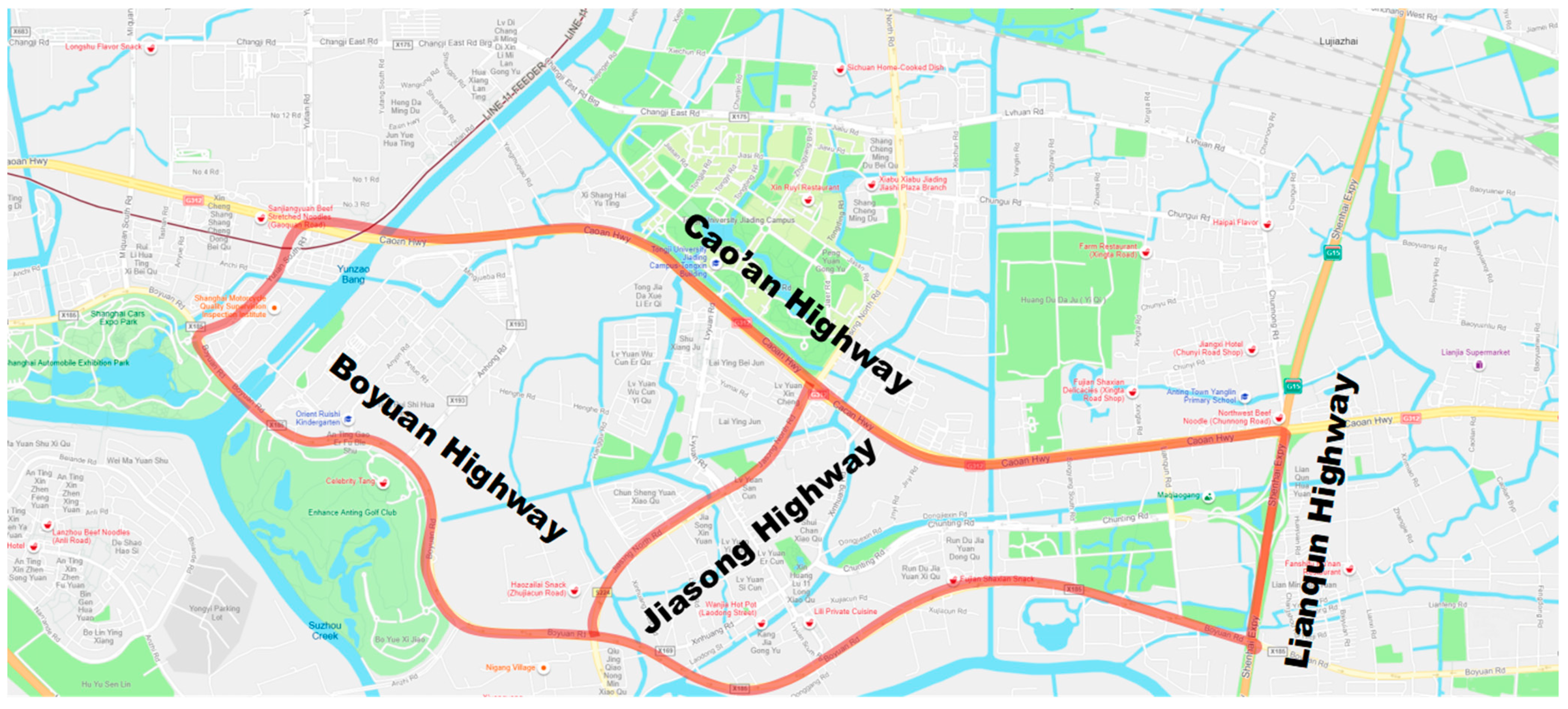
| Surface with slope: four samples Cao’an Highway Boyuan Highway | 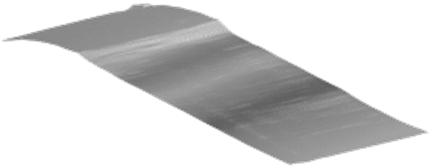 |
| Surface with rutting: four samples Jiasong Highway | 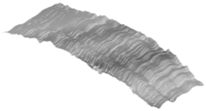 |
| Rough surface: three samples Lianqun Highway | 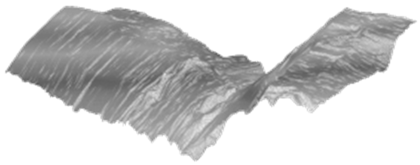 |
| Gallaway model | |
| USF model |
| Variable | Value |
|---|---|
| MTD | 1.0 mm |
| Tire pressure (Pt) | 250 Kpa |
| Wheel load (W) | 5000 N |
| SD | 1.0 |
| Tire tread depth | 1.0 mm |
Publisher’s Note: MDPI stays neutral with regard to jurisdictional claims in published maps and institutional affiliations. |
© 2022 by the authors. Licensee MDPI, Basel, Switzerland. This article is an open access article distributed under the terms and conditions of the Creative Commons Attribution (CC BY) license (https://creativecommons.org/licenses/by/4.0/).
Share and Cite
Yang, W.; Tian, B.; Fang, Y.; Wu, D.; Zhou, L.; Cai, J. Evaluation of Highway Hydroplaning Risk Based on 3D Laser Scanning and Water-Film Thickness Estimation. Int. J. Environ. Res. Public Health 2022, 19, 7699. https://doi.org/10.3390/ijerph19137699
Yang W, Tian B, Fang Y, Wu D, Zhou L, Cai J. Evaluation of Highway Hydroplaning Risk Based on 3D Laser Scanning and Water-Film Thickness Estimation. International Journal of Environmental Research and Public Health. 2022; 19(13):7699. https://doi.org/10.3390/ijerph19137699
Chicago/Turabian StyleYang, Wenchen, Bijiang Tian, Yuwei Fang, Difei Wu, Linyi Zhou, and Juewei Cai. 2022. "Evaluation of Highway Hydroplaning Risk Based on 3D Laser Scanning and Water-Film Thickness Estimation" International Journal of Environmental Research and Public Health 19, no. 13: 7699. https://doi.org/10.3390/ijerph19137699