
Revealing Impacts of Human Activities and Natural Factors on Dynamic Changes of Relationships among Ecosystem Services: A Case Study in the Huang-Huai-Hai Plain, China


 ,
, 
Abstract
:1. Introduction
2. Materials and Methods
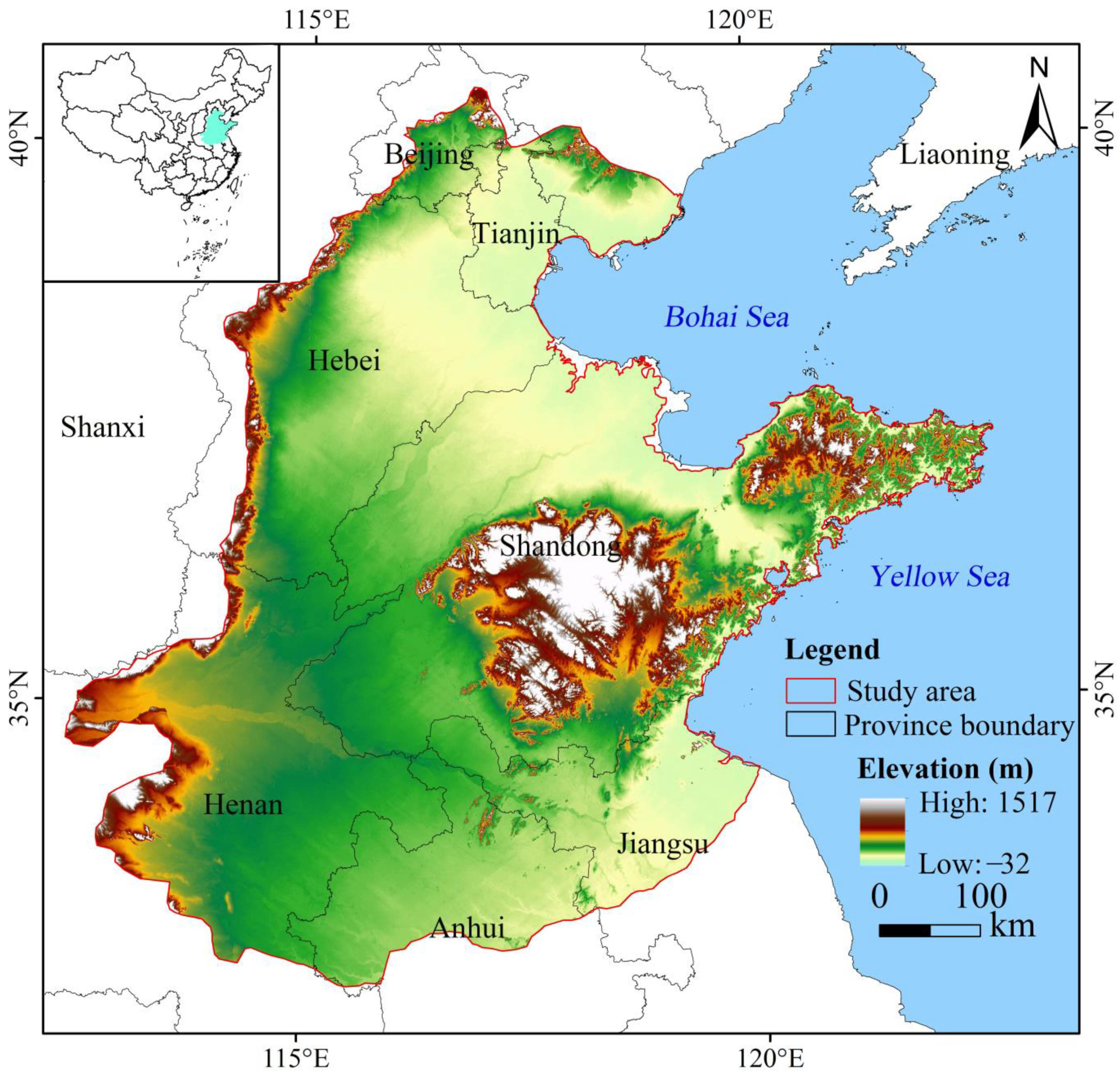
2.1. Study Area
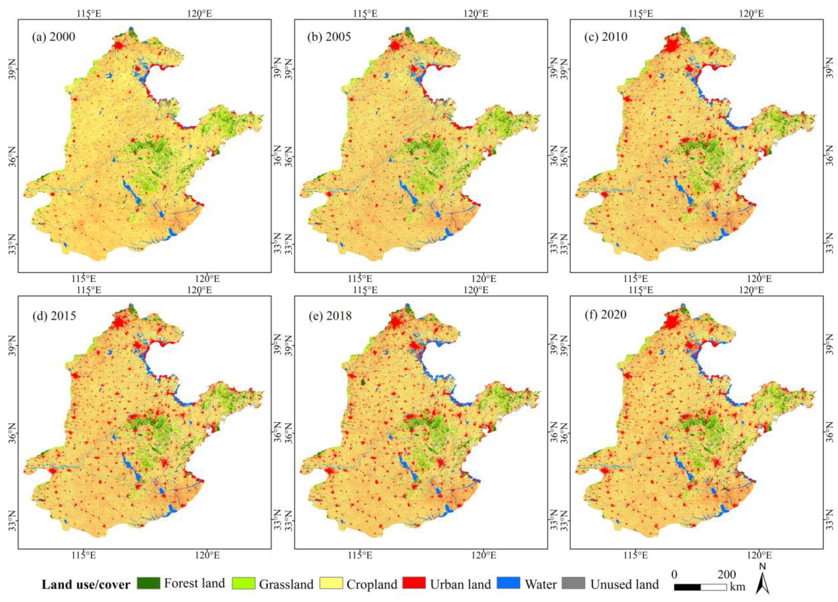
2.2. Data Sources
2.3. Modelling the ESs from 2000 to 2020
2.3.1. Net Primary Productivity
2.3.2. Food Production
2.3.3. Soil Conservation
2.3.4. Water Yield
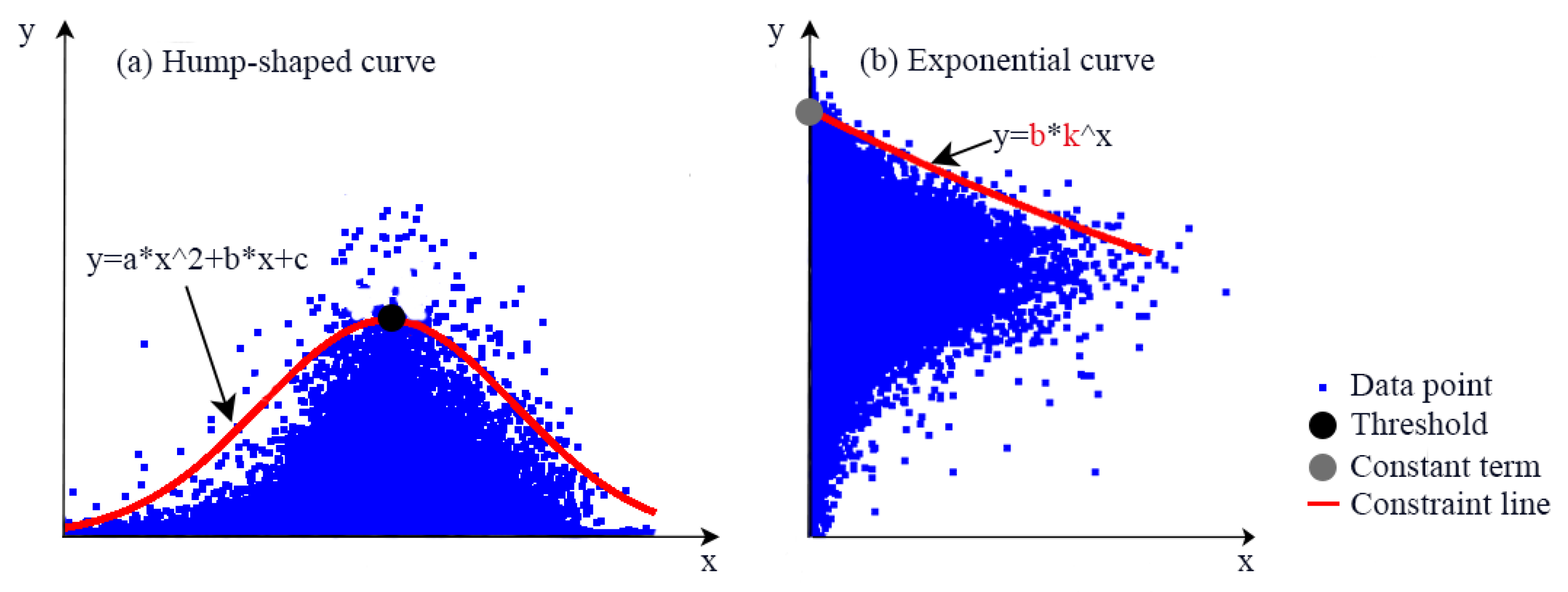
2.4. Extraction of the Constraint Lines between Paired ESs
2.5. Quantifying the Key Features of Constraint Effect among Paired ESs
2.6. Identifying Key Drivers and Their Interactive Effects on Relationships between Paired ESs from 2000 to 2020
3. Results
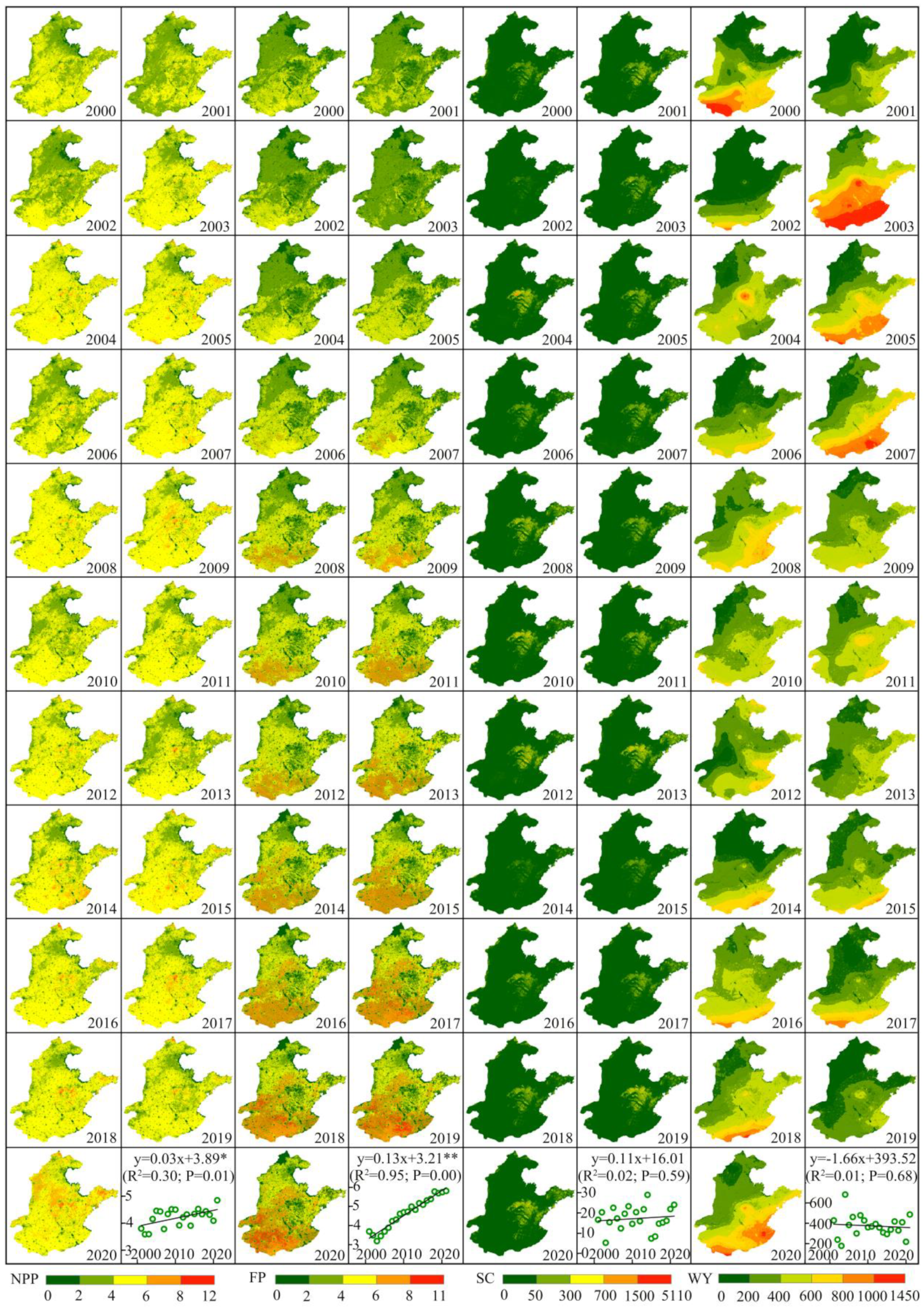
3.1. Spatiotemporal Patterns of ESs
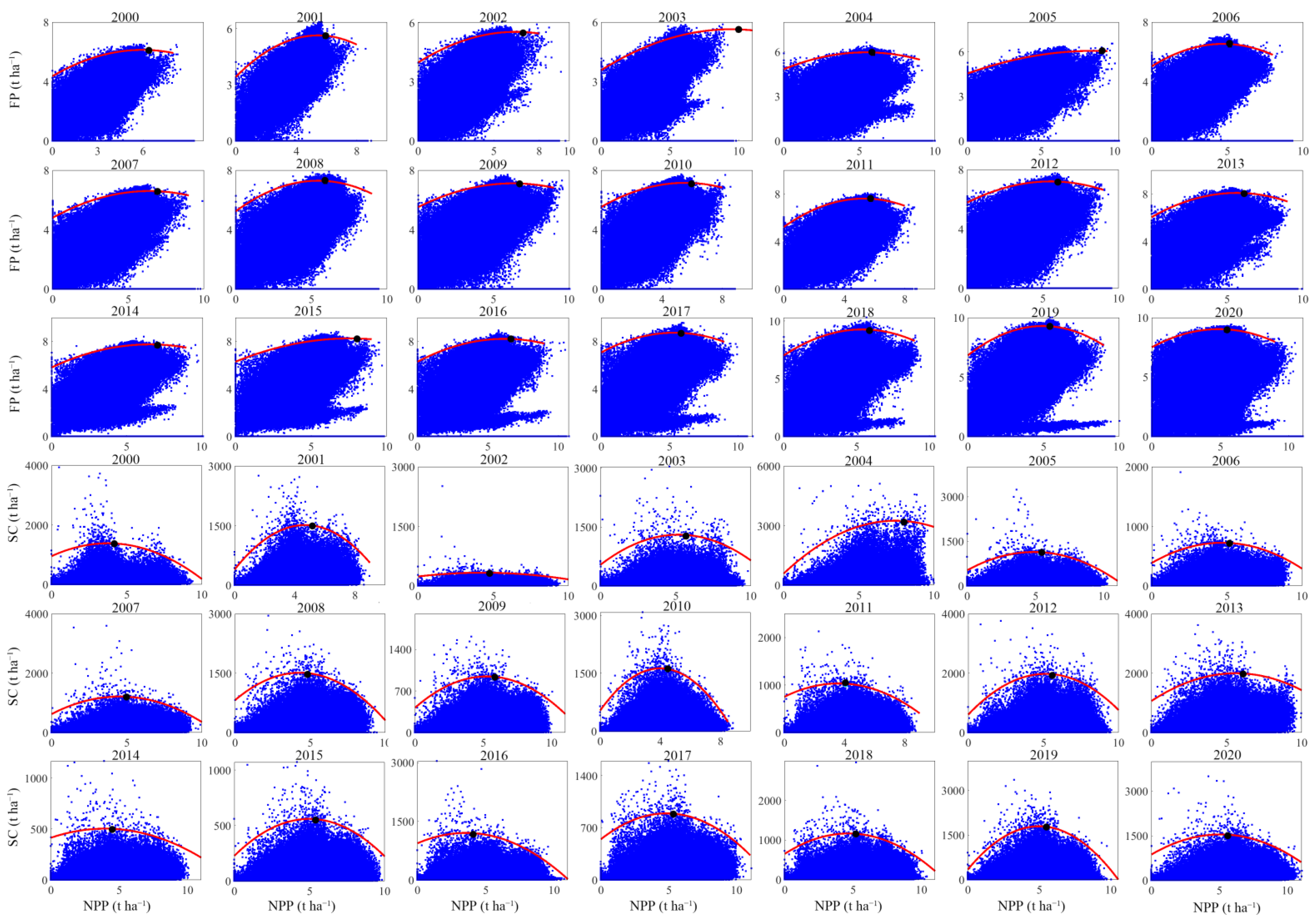
3.2. The Constraint Effect among Paired ESs from 2000 to 2020
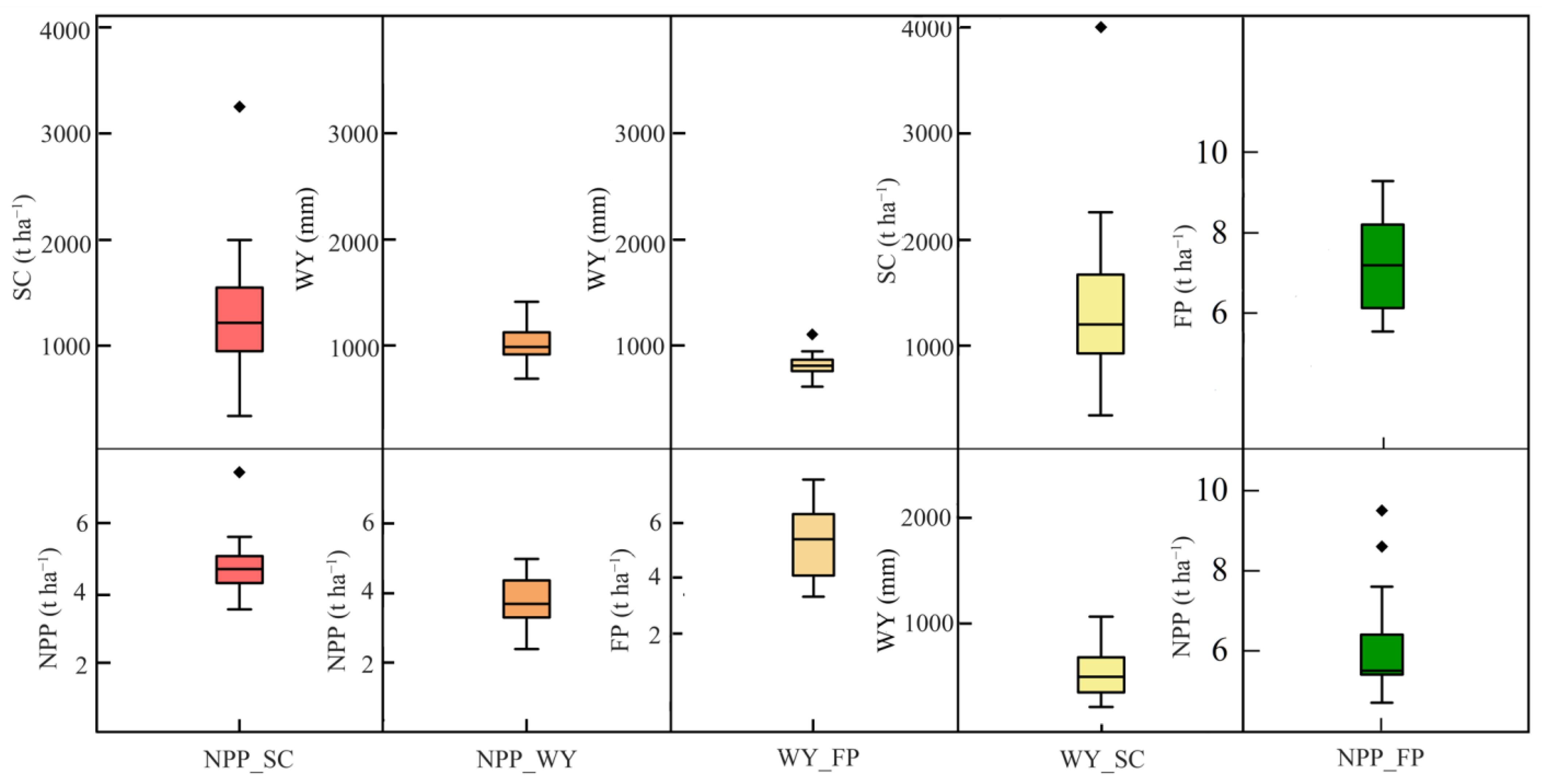
3.3. Key Features of the Constraint Lines among Paired ESs from 2000 to 2020
3.4. Effects of Driving Factors on the Constraint Relationship among Paired ESs
3.5. Interaction Effects of Socioeconomics and Landscape Configuration
4. Discussion
4.1. Mechanisms of Constraint Relationship among ESs
4.2. Effects of Influencing Factors on the Dynamic Change of Constraint Relationships among ESs
4.3. Implications for Ecosystem Management
5. Conclusions
Supplementary Materials
Author Contributions
Funding
Institutional Review Board Statement
Data Availability Statement
Acknowledgments
Conflicts of Interest
References
- Groot, R.; Alkemade, R.; Braat, L.; Hein, L.; Willemen, L. Challenges in integrating the concept of ecosystem services and values in landscape planning, management and decision making. Ecol. Complex. 2010, 7, 260–272. [Google Scholar] [CrossRef]
- Wu, J.G. Landscape sustainability science: Ecosystem services and human well-being in changing landscapes. Landsc. Ecol. 2013, 28, 999–1023. [Google Scholar] [CrossRef]
- Liang, J.; Li, S.; Li, X.D.; Li, X.; Liu, Q.; Meng, Q.F.; Lin, A.Q.; Li, J.J. Trade-off analyses and optimization of water-related ecosystem services (WRESs) based on land use change in a typical agricultural watershed, southern China. J. Clean. Prod. 2021, 279, 123851. [Google Scholar] [CrossRef]
- Jia, B.; Bi, J.; Hao, R.F.; Li, J.; Qiao, J.M. Identifying ecosystem states with patterns of ecosystem service bundles. Ecol. Indic. 2021, 131, 108195. [Google Scholar]
- Costanza, R.; Groot, R.D.; Paul, S.; Sander, P.; Van der Ploeg, S.; Anderson, S.J.; Ida, K.; Stephen, F.; Kerry, T.R. Changes in the global value of ecosystem services. Glob. Environ. Change 2014, 26, 152–158. [Google Scholar] [CrossRef]
- Li, S.K.; Li, X.B.; Dou, H.S.; Dang, D.L.; Gong, J.R. Integrating constraint effects among ecosystem services and drivers on seasonal scales into management practices. Ecol. Indic. 2021, 125, 107425. [Google Scholar] [CrossRef]
- Liu, L.M.; Wu, J.G. Ecosystem services-human wellbeing relationships vary with spatial scales and indicators: The case of China. Resour. Conserv. Recycl. 2021, 172, 105662. [Google Scholar] [CrossRef]
- Braun, D.; Damm, A.; Hein, L.; Petchey, O.L.; Schaepman, M.E. Spatio-temporal trends and trade-offs in ecosystem services: An Earth observation based assessment for Switzerland between 2004 and 2014. Ecol. Indic. 2018, 89, 828–839. [Google Scholar] [CrossRef]
- Qin, K.Y.; Li, J.; Yang, X.N. Trade-Off and Synergy among Ecosystem Services in the Guanzhong-Tianshui Economic Region of China. Int. J. Environ. Res. Public Health 2015, 12, 14094–14113. [Google Scholar] [CrossRef]
- Gou, M.; Li, L.; Ouyang, S.; Wang, N.; La, L.; Liu, C.; Xiao, W. Identifying and analying ecosystem service bundles and their socioecological drivers in the Three Gorges Reservoir Area. J. Clean. Prod. 2021, 307, 127208. [Google Scholar] [CrossRef]
- Kubiszewski, I.; Costanza, R.; Anderson, S.; Sutton, P. The future value of ecosystem services: Global scenarios and national implications. Ecosyst. Serv. 2017, 26, 289–301. [Google Scholar] [CrossRef]
- Raudsepp-Hearne, C.; Peterson, G.D.; Bennett, E.M. Ecosystem service bundles for analyzing tradeoffs in diverse landscapes. Proc. Natl. Acad. Sci. USA 2010, 107, 5242–5247. [Google Scholar] [CrossRef] [PubMed]
- Costanza, R.; Groot, R.d.; Braat, L.; Kubiszewski, I.; Fioramonti, L.; Sutton, P.; Farber, S.; Grasso, M. Twenty years of ecosystem services: How far have we come and how far do we still need to go? Ecosyst. Serv. 2017, 28, 1–16. [Google Scholar] [CrossRef]
- Li, J.D.; Lei, H.M. Tracking the spatio-temporal change of planting area of winter wheat-summer maize cropping system in the North China Plain during 2001–2018. Comput. Electron. Agric. 2021, 187, 106222. [Google Scholar] [CrossRef]
- Hao, R.F.; Yu, D.Y.; Wu, J.G. Relationship between paired ecosystem services in the grassland and agro-pastoral transitional zone of China using the constraint line method. Agric. Ecosyst. Environ. 2017, 240, 171–181. [Google Scholar] [CrossRef]
- Qiao, J.M.; Yu, D.Y.; Cao, Q.; Hao, R.F. Identifying the relationships and drivers of agro-ecosystem services using a constraint line approach in the agro-pastoral transitional zone of China. Ecol. Indic. 2019, 106, 105439. [Google Scholar] [CrossRef]
- Rukundo, E.; Liu, S.L.; Dong, Y.H.; Rutebuka, E.; Asamoah, E.F.; Xu, J.W.; Wu, X. Spatio-temporal dynamics of critical ecosystem services in response to agricultural expansion in Rwanda, East Africa. Ecol. Indic. 2018, 89, 696–705. [Google Scholar] [CrossRef]
- Peng, W.F.; Zhou, J.M.; Fan, S.Y.; Yang, C.J. Effects of the Land Use Change on Ecosystem Service Value in Chengdu, Western China from 1978 to 2010. J. Indian Soc. Remote Sens. 2015, 44, 197–206. [Google Scholar] [CrossRef]
- Liu, L.; Chen, X.; Chen, W.; Ye, X. Identifying the Impact of Landscape Pattern on Ecosystem Services in the Middle Reaches of the Yangtze River Urban Agglomerations, China. Int. J. Environ. Res. Public Health 2020, 17, 5063. [Google Scholar] [CrossRef]
- Chen, W.X.; Zeng, J.; Chu, Y.M.; Liang, J.L. Impacts of Landscape Patterns on Ecosystem Services Value: A Multiscale Buffer Gradient Analysis Approach. Remote Sens. 2021, 13, 2551. [Google Scholar] [CrossRef]
- Maestre, F.T.; Eldridge, D.J.; Soliveres, S.; Kefi, S.; Delgado-Baquerizo, M.; Bowker, M.A.; Garcia-Palacios, P.; Gaitan, J.; Gallardo, A.; Lazaro, R.; et al. Structure and functioning of dryland ecosystems in a changing world. Annu. Rev. Ecol. Evol. Syst. 2016, 47, 215–237. [Google Scholar] [CrossRef] [PubMed]
- Roodposhti, M.S.; Safarrad, T.; Shahabi, H. Drought sensitivity mapping using two one-class support vector machine algorithms. Atmos. Res. 2017, 193, 73–82. [Google Scholar] [CrossRef]
- Lin, T.; Xue, X.Z.; Shi, L.Y.; Gao, L.J. Urban spatial expansion and its impacts on island ecosystem services and landscape pattern: A case study of the island city of Xiamen, Southeast China. Ocean Coast. Manag. 2013, 81, 90–96. [Google Scholar] [CrossRef]
- Mao, D.H.; He, X.Y.; Wang, Z.M.; Tian, Y.L.; Xiang, H.X.; Yu, H.; Man, W.D.; Jia, M.M.; Ren, C.Y.; Zheng, H.F. Diverse policies leading to contrasting impacts on land cover and ecosystem services in Northeast China. J. Clean. Prod. 2019, 240, 117961. [Google Scholar] [CrossRef]
- Wang, Y.; Li, X.M.; Zhang, Q.; Li, J.F.; Zhou, X.W. Projections of future land use changes: Multiple scenarios-based impacts analysis on ecosystem services for Wuhan city, China. Ecol. Indic. 2018, 94, 430–445. [Google Scholar] [CrossRef]
- Zhang, Z.M.; Gao, J.F.; Fan, X.Y.; Lan, Y.; Zhao, M.S. Response of ecosystem services to socioeconomic development in the Yangtze River Basin, China. Ecol. Indic. 2017, 72, 481–493. [Google Scholar] [CrossRef]
- Qiao, X.N.; Gu, Y.Y.; Zou, C.X.; Xu, D.L.; Wang, L.; Ye, X.; Yang, Y.; Huang, X.F. Temporal variation and spatial scale dependency of the trade-offs and synergies among multiple ecosystem services in the Taihu Lake Basin of China. Sci. Total Environ. 2018, 651, 218–229. [Google Scholar] [CrossRef]
- Wu, X.; Qi, Y.; Shen, Y.J.; Yang, W.; Zhang, Y.; Kondoh, A. Change of winter wheat planting area and its impacts on groundwater depletion in the North China Plain. J. Geogr. Sci. 2019, 29, 891–908. [Google Scholar] [CrossRef]
- Zhang, D.; Huang, Q.; He, C.; Dan, Y.; Liu, Z. Planning urban landscape to maintain key ecosystem services in a rapidly urbanizing area: A scenario analysis in the Beijing-Tianjin-Hebei urban agglomeration, China. Ecol. Indic. 2018, 96, 559–571. [Google Scholar] [CrossRef]
- Wang, X.T.; Zhang, S.; Feng, L.L.; Zhang, J.H.; Deng, F. Mapping Maize Cultivated Area Combining MODIS EVI Time Series and the Spatial Variations of Phenology over Huanghuaihai Plain. Appl. Sci. 2020, 10, 2667. [Google Scholar] [CrossRef]
- Mw, A.; Ow, A.; Sla, B.; Ka, A. Temporal Variability in the Impacts of Particulate Matter on Crop Yields on the North China Plain. Sci. Total Environ. 2021, 776, 145135. [Google Scholar]
- Potter, C.S.; Randerson, J.T.; Field, C.B.; Matson, P.A.; Vitousek, P.M.; Mooney, H.A.; Klooster, S.A. Terrestrial ecosystem production: A process model based on global satellite and surface data. Glob. Biogeochem. Cycles 1993, 7, 811–841. [Google Scholar] [CrossRef]
- Feng, Y.H.; Zhu, J.X.; Zhao, X.; Tang, Z.Y.; Fang, J.Y. Changes in the trends of vegetation net primary productivity in China between 1982 and 2015. Environ. Res. Lett. 2019, 14, 124009. [Google Scholar] [CrossRef]
- Jian, P.; Lu, T.; Liu, Y.; Zhao, M.; Hu, Y.; Wu, J. Ecosystem services response to urbanization in metropolitan areas: Thresholds identification. Sci. Total Environ. 2017, 607–608, 706–714. [Google Scholar]
- Li, B.; Chen, N.; Wang, Y.; Wang, W. Spatio-temporal quantification of the trade-offs and synergies among ecosystem services based on grid-cells: A case study of Guanzhong Basin, NW China. Ecol. Indic. 2018, 94, 246–253. [Google Scholar] [CrossRef]
- Costanza, R.; D’Arge, R.; Groot, R.D.; Farber, S.; Grasso, M.; Hannon, B.; Limburg, K.; Naeem, S.; O’Neill, R.V.; Paruelo, J. The value of the world’s ecosystem services and natural capital. Ecol. Econ. 1997, 25, 3–15. [Google Scholar] [CrossRef]
- Renard, K.G.; Foster, G.R.; Weesies, G.A.; Porter, J.P. RUSLE: Revised universal soil loss equation. J. Soil Water Conserv. 1991, 46, 1–9. [Google Scholar]
- Peng, J.; Hu, X.; Wang, X.; Meersmans, J.; Liu, Y.; Qiu, S. Simulating the impact of Grain-for-Green Programme on ecosystem services trade-offs in Northwestern Yunnan, China. Ecosyst. Serv. 2019, 39, 100998. [Google Scholar] [CrossRef]
- Guo, Q.F.; Rundel, P.W. Self-thinning in early postfire chaparral succession: Mechanisms, implications, and a combined. Ecology 1998, 79, 579. [Google Scholar] [CrossRef]
- Thomson, J.D.; Weiblen, G.; Thomson, B.A.; Alfaro, S.; Legendre, P. Untangling Multiple Factors in Spatial Distributions: Lilies, Gophers, and Rocks. Ecology 1996, 77, 1689–1715. [Google Scholar] [CrossRef]
- Scharf, F.S.; Juanes, F.; Sutherland, M. Inferring Ecological Relationships from the Edges of Scatter Diagrams: Comparison of Regression Techniques. Ecology 1998, 79, 448–460. [Google Scholar] [CrossRef]
- Zhang, X.; Zhang, G.S.; Long, X.; Zhang, Q.; Liu, D.S.; Wu, H.J.; Li, S. Identifying the drivers of water yield ecosystem service: A case study in the Yangtze River Basin, China. Ecol. Indic. 2021, 132, 108304. [Google Scholar] [CrossRef]
- Deng, L.; Zhang, Q.; Cheng, Y.; Cao, Q.; Wang, Z.; Wu, Q.; Qiao, J. Underlying the influencing factors behind the heterogeneous change of urban landscape patterns since 1990: A multiple dimension analysis. Ecol. Indic. 2022, 140, 108967. [Google Scholar] [CrossRef]
- Karimi, J.D.; Corstanje, R.; Harris, J.A. Bundling ecosystem services at a high resolution in the UK: Trade-offs and synergies in urban landscapes. Landsc. Ecol. 2021, 36, 1817–1835. [Google Scholar] [CrossRef]
- Seidl, R.; Spies, T.A.; Peterson, D.L.; Stephens, S.L.; Hicke, J.A. Searching for resilience: Addressing the impacts of changing disturbance regimes on forest ecosystem services. J. Appl. Ecol. 2016, 53, 120–129. [Google Scholar] [CrossRef]
- Wissel, C. A universal law of the characteristic return time near thresholds. Oecologia 1984, 65, 101–107. [Google Scholar] [CrossRef]
- Wang, Q.; Wu, J.; Li, X.; Zhou, H.; Yang, J.; Geng, G.; An, X.; Liu, L.; Tang, Z. A comprehensively quantitative method of evaluating the impact of drought on crop yield using daily multi-scale SPEI and crop growth process model. Int. J. Biometeorol. 2017, 61, 685–699. [Google Scholar] [CrossRef]
- Hao, R.F.; Yu, D.Y.; Sun, Y.; Shi, M.C. The features and influential factors of interactions among ecosystem services. Ecol. Indic. 2019, 101, 770–779. [Google Scholar] [CrossRef]
- Wright, R.J.; Boyer, D.G.; Winant, W.M.; Perry, H.D. The influence of soil factors on yield differences among landscape positions in an Appalachian cornfield. Soil Sci. 1990, 149, 375–382. [Google Scholar] [CrossRef]
- Gomes, L.C.; Bianchi, F.J.J.A.; Cardoso, I.M.; Schulte, R.P.O.; Fernandes, R.B.A.; Fernandes, F.E.I. Disentangling the historic and future impacts of land use changes and climate variability on the hydrology of a mountain region in Brazil. J. Hydrol. 2020, 594, 125650. [Google Scholar] [CrossRef]
- Lang, Y.; Song, W.; Zhang, Y. Responses of the water-yield ecosystem service to climate and land use change in Sancha River Basin, China. Phys. Chem. Earth 2017, 101, 102–111. [Google Scholar] [CrossRef]
- Liu, S.; Mo, X.; Lin, Z.; Xu, Y.; Ji, J.; Wen, G.; Richey, J. Crop yield responses to climate change in the Huang-Huai-Hai Plain of China. Agric. Water Manag. 2010, 97, 1195–1209. [Google Scholar] [CrossRef]
- Tang, Z.L.; Sun, G.; Zhang, N.N.; He, J.; Wu, N. Impacts of Land-Use and Climate Change on Ecosystem Service in Eastern Tibetan Plateau, China. Sustainability 2018, 10, 467. [Google Scholar] [CrossRef]
- Zang, Z.; Zou, X.; Zuo, P.; Song, Q.; Wang, C.; Wang, J. Impact of landscape patterns on ecological vulnerability and ecosystem service values: An empirical analysis of Yancheng Nature Reserve in China. Ecol. Indic. 2017, 72, 142–152. [Google Scholar] [CrossRef]
- Hou, L.; Wu, F.; Xie, X. The spatial characteristics and relationships between landscape pattern and ecosystem service value along an urban-rural gradient in Xi’an city, China. Ecol. Indic. 2020, 108, 105720. [Google Scholar] [CrossRef]
- Wu, X.; Cai, X.; Li, Q.; Ren, B.; Bi, Y.; Zhang, J.; Wang, D. Effects of Nitrogen Application Rate on Summer Maize (Zea mays L.) Yield and Water–Nitrogen Use Efficiency under Micro–Sprinkling Irrigation in the Huang–Huai–Hai Plain of China. 2021. Available online: https://www.tandfonline.com/doi/abs/10.1080/03650340.2021.1939867 (accessed on 1 May 2022).
- Li, W.; Zinda, J.A.; Zhang, Z. Does the “Returning Farmland to Forest Program” Drive Community-Level Changes in Landscape Patterns in China? Forests 2019, 10, 933. [Google Scholar] [CrossRef]
- Xian, J.; Xia, C.; Cao, S. Cost–benefit analysis for China’s Grain for Green Program. Ecol. Eng. 2020, 151, 105850. [Google Scholar] [CrossRef]
- Wang, B.; Gao, P.; Niu, X.; Sun, J.N. Policy-driven China’s Grain to Green Program: Implications for ecosystem services. Ecosyst. Serv. 2017, 27, 38–47. [Google Scholar] [CrossRef]
- Wang, B.; Tang, H.; Xu, Y. Integrating ecosystem services and human well-being into management practices: Insights from a mountain-basin area, China. Ecosyst. Serv. 2017, 27, 58–69. [Google Scholar] [CrossRef]
- Liu, B.Y.; Nearing, M.A.; Risse, L.M. Slope Length Effects on Soil Loss for Steep Slopes. Soil Sci. Soc. Am. J. 2000, 64, 1759–1763. [Google Scholar] [CrossRef]
- Xu, Y.J.; Yao, Z.H.; Zhao, D.B. Estimating Soil Erosion in North China Plain Based on RS/GIS and RUSLE. Bull. Soil Water Conserv. 2012, 32, 217–221. [Google Scholar]


| Data | Data Description (Unit) | Data Source |
|---|---|---|
| Meteorological data | Daily mean temperature (°C) | China Meteorological Sharing Service System |
| Daily rainfall (mm) | ||
| Daily sunshine duration (h) | ||
| Digital Elevation Model (DEM) | The Shuttle Radar Topography Mission (SRTM) digital elevation model with 90-m spatial resolution (m) | Geospatial Data Cloud (https://www.gscloud.cn/home, accessed on 1 October 2020) |
| Soil data | HWSD (v1.1) soil dataset (including fractions of sand, silt, clay and organic carbon in the topsoil and soil depth) | Cold and Arid Regions Science Data Center at Lanzhou |
| Land use/cover | Land use/cover in 2000, 2005, 2010, 2015, and 2018 at 30-m spatial resolution, and 2020 at 250-m spatial resolution | Resource and Environment Science and Data Center |
| Normalized Difference Vegetation Index (NDVI) | MODIS NDVI product (250 mm resolution MOD13Q1 product) | NASA |
| Crop yield | The crop yield of staple food crops for each city | Statistical yearbook |
| Socio economic data | Gross Domestic Product (GDP)_ | Resource and Environment Science and Data Center (https://www.resdc.cn/, accessed on 2 December 2021) |
| Population | World Pop (https://www.worldpop.org/, accessed on 2 December 2021) |
| Data | Data Description |
|---|---|
| Climatic factors | Average precipitation (mm) |
| Average temperature (°C) | |
| Vegetation factor | Normalized Difference Vegetation Index |
| Landscape composition | The total area of cropland (%) |
| The total area of forest land (%) | |
| The total area of grassland (%) | |
| The total area of water (%) | |
| The total area of urban land (%) | |
| The total area of unused land (%) | |
| Landscape configuration | Perimeter-Area Fractal Dimension |
| Landscape Shape Index | |
| Contagion (%) | |
| Shannon’s Diversity Index | |
| Patch Density (Unit/100 ha) | |
| Socio-economic factors | GDP (CYN) |
| Population (person) |
| NPP_FP | NPP_SC | SC_FP | NPP_WY | WY_FP | WY_SC | |
|---|---|---|---|---|---|---|
| 2000 | 0.79 ** | 0.21 ** | 0.77 ** | 0.94 ** | 0.75 ** | 0.41 ** |
| 2001 | 0.80 ** | 0.56 ** | 0.73 ** | 0.88 ** | 0.43 ** | 0.61 ** |
| 2002 | 0.84 ** | 0.13 ** | 0.52 ** | 0.91 ** | 0.41 ** | 0.40 ** |
| 2003 | 0.90 ** | 0.22 ** | 0.72 ** | 0.93 ** | 0.73 ** | 0.56 ** |
| 2004 | 0.63 ** | 0.38 ** | 0.84 ** | 0.51 ** | 0.82 ** | 0.91 ** |
| 2005 | 0.86 ** | 0.38 ** | 0.78 ** | 0.95 ** | 0.79 ** | 0.44 ** |
| 2006 | 0.71 ** | 0.30 ** | 0.70 ** | 0.95 ** | 0.72 ** | 0.75 ** |
| 2007 | 0.81 ** | 0.31 ** | 0.66 ** | 0.96 ** | 0.42 ** | 0.66 ** |
| 2008 | 0.76 ** | 0.49 ** | 0.80 ** | 0.89 ** | 0.77 ** | 0.68 ** |
| 2009 | 0.85 ** | 0.38 ** | 0.77 ** | 0.93 ** | 0.63 ** | 0.66 ** |
| 2010 | 0.76 ** | 0.75 ** | 0.89 ** | 0.91 ** | 0.67 ** | 0.66 ** |
| 2011 | 0.87 ** | 0.28 ** | 0.87 ** | 0.89 ** | 0.79 ** | 0.58 ** |
| 2012 | 0.78 ** | 0.38 ** | 0.76 ** | 0.89 ** | 0.67 ** | 0.80 ** |
| 2013 | 0.82 ** | 0.33 ** | 0.66 ** | 0.80 ** | 0.63 ** | 0.67 ** |
| 2014 | 0.81 ** | 0.17 ** | 0.62 ** | 0.89 ** | 0.59 ** | 0.54 ** |
| 2015 | 0.82 ** | 0.47 ** | 0.83 ** | 0.92 ** | 0.74 ** | 0.57 ** |
| 2016 | 0.80 ** | 0.50 ** | 0.76 ** | 0.95 ** | 0.74 ** | 0.59 ** |
| 2017 | 0.64 ** | 0.42 ** | 0.78 ** | 0.94 ** | 0.64 ** | 0.77 ** |
| 2018 | 0.77 ** | 0.44 ** | 0.67 ** | 0.96 ** | 0.42 ** | 0.62 ** |
| 2019 | 0.79 ** | 0.67 ** | 0.71 ** | 0.89 ** | 0.66 ** | 0.77 ** |
| 2020 | 0.82 ** | 0.30 ** | 0.76 ** | 0.97 ** | 0.58 ** | 0.56 ** |
| Thresholds | Slopes (k) and Constant Terms (b) | |||||||||||
|---|---|---|---|---|---|---|---|---|---|---|---|---|
| NPP_SC | NPP_WY | WY_SC | WY_FP | NPP_FP | SC_FP | |||||||
| NPP | SC | FP | WY | WY | SC | WY | FP | NPP | FP | k | b | |
| 2000 | 3.75 | 1386.35 | 3.54 | 1379.62 | 554.12 | 1183.14 | 587.20 | 5.91 | 6.00 | 6.13 | 0.9995 | 6.53 |
| 2000 | 4.68 | 1517.80 | 4.12 | 803.00 | 460.27 | 1611.79 | 367.30 | 5.72 | 5.40 | 5.64 | 0.9997 | 5.60 |
| 2002 | 4.29 | 332.45 | 3.96 | 978.35 | 300.01 | 338.98 | 424.20 | 5.50 | 6.50 | 5.54 | 0.9991 | 6.02 |
| 2003 | 5.19 | 1306.24 | 3.49 | 1439.64 | 1021.36 | 1296.03 | 884.70 | 5.25 | 9.50 | 5.64 | 0.9997 | 5.62 |
| 2004 | 7.45 | 3254.79 | 2.88 | 1100.41 | 1038.03 | 4006.01 | 402.50 | 5.91 | 5.40 | 5.96 | 0.9998 | 5.64 |
| 2005 | 4.88 | 1139.83 | 4.04 | 1146.43 | 761.87 | 1197.49 | 684.80 | 6.02 | 8.60 | 6.06 | 0.9997 | 6.34 |
| 2006 | 4.69 | 725.93 | 4.06 | 954.79 | 321.33 | 695.95 | 486.40 | 6.72 | 4.70 | 6.53 | 0.9995 | 6.80 |
| 2007 | 4.53 | 1212.90 | 4.00 | 1218.52 | 784.28 | 1301.24 | 555.80 | 6.93 | 6.40 | 6.59 | 0.9997 | 6.95 |
| 2008 | 4.31 | 1510.45 | 4.56 | 962.81 | 652.23 | 1669.39 | 614.10 | 7.37 | 5.40 | 7.29 | 0.9997 | 7.18 |
| 2009 | 5.25 | 945.13 | 4.61 | 772.81 | 418.19 | 884.83 | 470.10 | 7.14 | 6.30 | 7.11 | 0.9996 | 7.28 |
| 2010 | 3.99 | 1627.28 | 4.77 | 781.59 | 468.34 | 1572.66 | 453.30 | 7.27 | 5.50 | 7.15 | 0.9997 | 7.09 |
| 2011 | 3.61 | 1033.68 | 4.75 | 927.59 | 582.29 | 1066.09 | 505.50 | 7.73 | 5.30 | 7.61 | 0.9996 | 7.39 |
| 2012 | 5.15 | 1975.39 | 4.68 | 916.55 | 599.66 | 2183.67 | 517.50 | 7.33 | 5.50 | 7.19 | 0.9998 | 7.11 |
| 2013 | 5.61 | 1996.45 | 4.88 | 696.88 | 473.73 | 2257.91 | 270.80 | 8.29 | 5.60 | 8.09 | 0.9998 | 8.24 |
| 2014 | 3.95 | 504.21 | 4.57 | 1025.30 | 301.90 | 478.84 | 517.10 | 7.81 | 6.60 | 7.74 | 0.9993 | 8.17 |
| 2015 | 4.98 | 559.82 | 4.69 | 1006.75 | 373.17 | 527.14 | 468.90 | 8.24 | 7.60 | 8.25 | 0.9993 | 8.28 |
| 2016 | 3.54 | 1202.79 | 4.76 | 1042.39 | 183.32 | 1173.02 | 587.00 | 8.25 | 6.20 | 8.21 | 0.9995 | 8.61 |
| 2017 | 4.84 | 893.33 | 5.73 | 1042.21 | 259.75 | 924.20 | 525.70 | 8.86 | 5.40 | 8.72 | 0.9996 | 8.82 |
| 2018 | 4.66 | 1165.07 | 6.08 | 1200.92 | 191.20 | 1039.53 | 544.70 | 9.49 | 5.40 | 9.27 | 0.9995 | 9.91 |
| 2019 | 4.97 | 1795.86 | 5.98 | 693.92 | 420.26 | 1989.14 | 286.70 | 9.38 | 5.00 | 9.30 | 0.9998 | 8.72 |
| 2020 | 5.06 | 1545.14 | 6.07 | 1194.82 | 760.21 | 1742.78 | 594.80 | 9.16 | 4.90 | 9.03 | 0.9998 | 9.01 |
| Trend | ↓ | ↓ | ↑ ** | ↓ | ↓ | ↓ | ↓ | ↑ ** | ↓ | ↑ ** | ↑ | ↑ ** |
| Thresholds | k | b | |||||||||||||
|---|---|---|---|---|---|---|---|---|---|---|---|---|---|---|---|
| NPP_FP | NPP_SC | WY_SC | NPP_WY | WY_FP | SC_FP | ||||||||||
| NPP | FP | NPP | SC | WY | SC | NPP | WY | WY | FP | ||||||
| Model | 0 | 0 | 0 | 0 | 0 | 1 | 0 | 0 | 0 | 1 | 0 | 0 | 0 | 0 |  |
| Accuracy (%) | 40.9 | 95.7 | 99.9 | 100.0 | 91.9 | 91.9 | 100.0 | 94.2 | 82.4 | 82.4 | 92.0 | 70.0 | 39.1 | 94.2 | |
| NDVI | 0.12 | −2.1 ** | 0.3 | 0.3 | −3.7 ** | 1.8 ** | 0.4 * | ||||||||
| PPT | 0.7 * | −0.2 | 1.4 * | 0.2 | 0.2 | −2.4 ** | 1.0 ** | 1.0 ** | 0.9 ** | 0.1 | |||||
| TEM | −0.4 | −1.6 * | −0.4 ** | −0.4 ** | 0.8 * | 0.8 * | −0.1 | ||||||||
| population | 0.6 | −4.3 * | 6.2 ** | −6.8 * | −6.8 * | 3.7 | −1.3 | ||||||||
| GDP | 0.3* | 3.0 * | 3.0 * | 7.6 * | −3.5 * | 1.6 * | |||||||||
| Area(cropland) | −1.0 ** | ||||||||||||||
| Area(water) | −1.4 * | 0.8 ** | 0.8 ** | ||||||||||||
| Area(forest) | −1.4 ** | −0.6 | −1.2 ** | ||||||||||||
| Area(unusedland) | −1.4 | 0.3 * | 1.1 * | ||||||||||||
| CONTAG | −8.8 * | −8.8 * | |||||||||||||
| LSI | 1.9 * | −13.5 * | −13.5 * | ||||||||||||
| PARFAC | −0.8 | 1.0 ** | −4.0 | −3.5 | 8.6 * | 8.6 * | 0.9 ** | ||||||||
| Interaction effects | |||||||||||||||
| Population *PAFRAC | −4.4 * | ||||||||||||||
| GDP*PAFRAC | 1.3 * | ||||||||||||||
Publisher’s Note: MDPI stays neutral with regard to jurisdictional claims in published maps and institutional affiliations. |
© 2022 by the authors. Licensee MDPI, Basel, Switzerland. This article is an open access article distributed under the terms and conditions of the Creative Commons Attribution (CC BY) license (https://creativecommons.org/licenses/by/4.0/).
Share and Cite
Deng, L.; Li, Y.; Cao, Z.; Hao, R.; Wang, Z.; Zou, J.; Wu, Q.; Qiao, J. Revealing Impacts of Human Activities and Natural Factors on Dynamic Changes of Relationships among Ecosystem Services: A Case Study in the Huang-Huai-Hai Plain, China. Int. J. Environ. Res. Public Health 2022, 19, 10230. https://doi.org/10.3390/ijerph191610230
Deng L, Li Y, Cao Z, Hao R, Wang Z, Zou J, Wu Q, Qiao J. Revealing Impacts of Human Activities and Natural Factors on Dynamic Changes of Relationships among Ecosystem Services: A Case Study in the Huang-Huai-Hai Plain, China. International Journal of Environmental Research and Public Health. 2022; 19(16):10230. https://doi.org/10.3390/ijerph191610230
Chicago/Turabian StyleDeng, Longyun, Yi Li, Zhi Cao, Ruifang Hao, Zheye Wang, Junxiao Zou, Quanyuan Wu, and Jianmin Qiao. 2022. "Revealing Impacts of Human Activities and Natural Factors on Dynamic Changes of Relationships among Ecosystem Services: A Case Study in the Huang-Huai-Hai Plain, China" International Journal of Environmental Research and Public Health 19, no. 16: 10230. https://doi.org/10.3390/ijerph191610230
APA StyleDeng, L., Li, Y., Cao, Z., Hao, R., Wang, Z., Zou, J., Wu, Q., & Qiao, J. (2022). Revealing Impacts of Human Activities and Natural Factors on Dynamic Changes of Relationships among Ecosystem Services: A Case Study in the Huang-Huai-Hai Plain, China. International Journal of Environmental Research and Public Health, 19(16), 10230. https://doi.org/10.3390/ijerph191610230