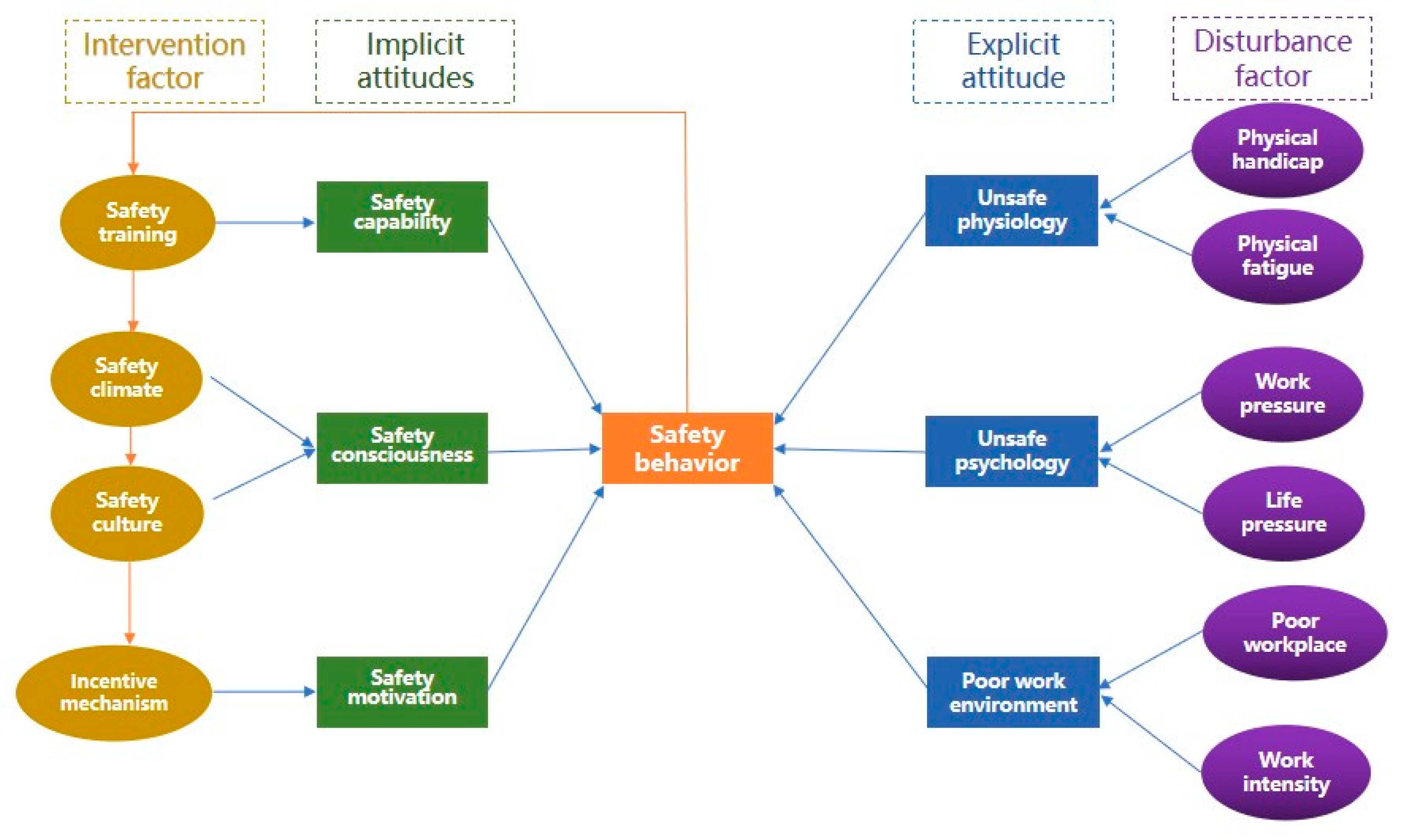
3.2. Simulation Model Construction
The variables in the model were qualitative; therefore, they were measured in dimensionless units and represented by the unit “1”. The safe behavior value was recorded daily as a real-time dynamic variable. Its value is affected by the positive effect value and negative effect value of the day, and its system dynamics equation can be expressed as:
The value of SBPV is affected by implicit factors, and its system dynamics equation can be expressed as:
The value of SPNV is affected by explicit factors, and its system dynamics equation can be expressed as:
where X
i (
i = 1, 2, …
n) is the parameter of the system dynamics equation and σ
i (
i = 1, 2 …
n) is various error terms, the same as below.
System dynamics is based on feedback loops; therefore, it is insensitive to most non-critical parameters in the model. As long as the parameter estimation is within a reasonable range, there will be little or no deviation in the model results [
27]. Therefore, the influence of the error term σ
i(
i = 1, 2, …
n) was not considered in this study, and its value was set to 0, the same as below.
Next, we analyzed the disturbance factors. We defined physical handicap as a dynamic variable because a worker’s health status varies daily. It is real-time rather than cumulative. The same applies for other disturbances such as changing work sites, less work completed that day, etc. Here, we assigned a value to it every day by cyclic Event 1 (see
Appendix A for the properties of Event
i (
i = 1, 2, 3, 4, 5, 6, 7)). In addition, considering that variables of the system dynamics module and variables in discrete events cannot be used together, another variable was introduced under the agent module and made equal. It can be expressed as:
ST1, SCL1, CSU1, IM1, SCA1, SCAD1, SCO1, SCOD1, SM1, SMD1, PF1, WP1, LP1, PW1, and WI1 are the same.
Explicit factors directly affected by disturbance factors are also real-time dynamic variables, and the system dynamics equations between them can be expressed as:
Considering the impacts of cost, schedule, and other factors, safety training and other intervention factors cannot be performed frequently. Input values are only available when the interventions occur; thus, we defined them as real-time dynamic variables. Two interventions were established in this study, and the duration of the intervention was one day. One was active intervention, a periodic intervention, i.e., where the managers intervened in the system once a month on the first day. The second kind was passive intervention, which was an irregular intervention. When the safety behavior value of the preceding month was less than 0.2, this meant that the safety attitude of workers was poor and the frequency of unsafe behavior was high, and the managers intervened in the system once on the first day of the following month.
In the active intervention model, we assigned values to the intervention factors by cyclic Event 2 and controlled the duration of the intervention by cyclic Event 3.
In the passive intervention model, we assigned values to the intervention factors by cyclic Event 4 and controlled the duration of the intervention by cyclic Event 3.
Each of the implicit factors increased with an input value when the interventions were triggered. We considered that their values during the two interventions were not invariable and would decay with time until the next intervention was triggered at a new rate. Therefore, they are cumulative stocks. Each implicit factor had corresponding increases and decreases, and their system dynamics equations are:
The values here may be greater than 1; therefore, we set cyclic Event 5 to control it.
The system dynamics equations between the increase in each implicit factor and its corresponding intervention factors can be expressed as:
In the initial stage of the system, considering that each unit had intervention measures such as pre-entry training, we took the value of the first intervention transformed by the above equation as the initial value of each implicit factor. The attenuation effect of each implicit factor had not yet come into play; therefore, the reduction in each implicit factor was 0. Therefore, the initial value of each implicit factor was equal to the increase in each implicit factor at this time.
For the decay of implicit factors, we introduced the formula of the memory forgetting curve [
28] as the effect of their decay over time. It can be expressed as:
where
R is the retrievability (a measure of how easy it is to retrieve a piece of information from memory),
S is the stability of memory (which determines how fast
R falls over time in the absence of training, testing, or other recall), and
t is time.
Memory strength will increase after each intervention; therefore, a new round of slower decay is caused. It was supposed that the decay rate decreased by Z to the power of H (0 < Z < 1, H = 1, 2, … n), where H was the number of interventions. The reduction in each implicit factor was controlled by cyclic Event 6.
In the passive intervention model, the values of safety behavior could remain above 0.2 for a long time after several interventions (where the level of values is slightly greater than 0.2), during which there are no intervention measures, making workers relaxed and idle. In this regard, we introduced the complete forgetting mechanism. When there was no intervention for more than 60 consecutive days, its attenuation rate became the initial state, controlled by cyclic Event 7.
3.3. Meta-Analysis
As mentioned above, we used meta-analysis to merge the correlation coefficients of previous studies as parameters of the system dynamics equation in the simulation model.
In this study, meta-analysis recommended by Hunter and Schmidt [
22] was used to merge effect values from the related literature. There are four steps in meta-analysis: (a) literature search; (b) literature selection; (c) literature coding; and (d) data analysis. To provide information on the estimate of population correlation, we report the study number (K); total sample size (N); uncorrected correlation value (r), which is sample size-weighted; the corrected correlation value (r
c), which is sample size-weighted and reliability-corrected; and the 95% confidence interval for r
c (95%CI).
3.3.1. Literature Search
Several retrieval techniques were adopted to ensure that the literature and samples included in the study were maximized, complete, and representative. First, considering timeliness, a span of 11.5 years was chosen for the literature search: from 1 January 2010 to 30 June 2021. Second, we searched the China National Knowledge Infrastructure (CNKI), the largest Chinese document database, and Web of Science, the largest international database. In addition, we used the keywords “construction” and “unsafe/safety behavior”. Finally, we have checked the literature we obtained manually to avoid missing some related studies.
3.3.2. Literature Selection
After completing the literature search, we obtained 691 research articles and applied some inclusion and exclusion criteria to filter the existing literature further. First, the study had to be based on empirical research and needed to report the coding details, such as the sample size (n), correlation value (r), or other effect sizes (e.g., standardized multiple regression coefficients (β), t for t-test, F for F-test), which can be easily converted to r. Then, we excluded articles that: (a) presented qualitative or non-empirical research; (b) ambiguously defined their factors and presented relationships between factors; or (c) were less reliable or were of poor quality. Finally, 17 articles were retained for coding.
3.3.3. Literature Coding
For each article, the coded information is listed as the article ID (number), author, publication date, title, article source, sample size (N), independent and dependent variables, and the correlation value r or other effect size between variables.
3.3.4. Data Analysis
It was supposed that (X
1, Y
1), (X
2, Y
2), …, (X
n, Y
n) were randomly sampled from a population with a mean of (μ
1, μ
2), variance of (
), and correlation value of
. For large samples, the following distribution was found [
29]:
where
r is the correlation value of the sample of two variables and
is the correlation value of the population of two variables. The actual correlation value of the population of two variables,
, was unknown; thus, it was generally estimated by the correlation value of sample
r. The variance of the two values
can be approximately estimated as [
30]:
The combination of correlation value
r follows the general combination process of effect size [
29,
31].
It is assumed that all the correlation values are from the same population:
where
is unknown and can be estimated by the estimator
:
where
Wi is the weight of the Study
i, and
ri is the effect size of the Study
i.
Variance reflects whether the measurement index is accurate or not, so the mutual variance of each study
can be used to represent the weight
Wi of each study:
is unknown and can be estimated by the variance of each sample
; then, the estimator
can be expressed as:
where
ri is the correlation value of Study
i.
Its variance,
, can be expressed as:
The significance,
Z, of the combined estimator,
, can be tested as:
Then, the confidence interval of the actual value of the combined estimator,
, is:


