Survival of Frail Elderly with Delirium

Abstract

This study aims to determine when frailty increases the risks of delirium mortality. Hospital patients falling into the elderly frail or pre-frail category were recruited, some without delirium, some with delirium at admission, and some who developed delirium during admission. We screened for frailty, cognitive status, and co-morbidities whenever possible and extracted drug information and mortality data from electronic health records. Kaplan–Meier estimates of survival probability functions were computed at four times, comparing delirium versus non delirium patients. Differences in survival were assessed by a log-rank test. Independent Cox’s regression was carried out to identify significant hazard risks (HR) at 1 month, 6 months, 1 year, and 2 years. Delirium predicted mortality (log-rank test, p < 0.0001) at all four censoring points. Variables with significant HRs were frailty indicators, comorbidities, polypharmacy, and the use of specific drugs. For the delirium cohort, variables with the most significant 2-year hazard risks (HR(95%CI)) were: male gender (0.43 20 (0.26,0.69)), weight loss (0.45 (0.26,0.74)), sit and stand up test (0.67 (0.49,0.92)), readmission within 30 days of discharge (0.50 (0.30,0.80)), cerebrovascular disease (0.45 (0.27,0.76)), head trauma (0.54 22 (0.29,0.98)), number of prescribed drugs (1.10 (1.03,1.18)), and the use of diuretics (0.57 (0.34,0.96)). These results suggest that polypharmacy and the use of diuretics increase mortality in frail elderly patients with delirium.

1. Introduction

Delirium is a severe psychiatric syndrome characterized by a sharp change in attention, awareness, and the cognitive state of the patient [1,2,3] that is highly prevalent in hospitalized older patients [4], and it is a common complication after surgery [5,6,7]. In older people, the most frequent presentation of delirium is hypoactive [8], showing psychomotor slow down, bradypsychia, slow language, apathy, and inhibition. Most frequent precipitating factors in community-dwelling older individuals are infectious diseases, followed by drugs and hydro-electrolytic disorders [9]. Machine learning tools have been proposed for the identification of delirium onset risk factors [10,11]. The duration of delirium is variable, persisting for weeks or months in 20% of patients with dementia [12], which is a high risk factor for delirium in older patients [13], while delirium onset often leads to cognitive deterioration and dementia [3,14,15]. There is a strong relation between frailty [16,17,18,19] and delirium in older patients [20], with frailty identified as a predictor of delirium [21,22] and delirium onset as a strong biomarker for underlying frailty in older adults [23].

Delirium prevalence is highly variable depending on the study, population, and environmental conditions [24,25,26]. Delirium is the second most prevalent psychiatric syndrome in the hospital environment [27]. In the older population, delirium carries higher mortality risks, longer hospital stays, and impedes cognitive and functional capabilities [28]. An estimated 20% of hospitalized patients over 65 years in the US suffer complications due to delirium [29]. A recent study carried out over three emergency departments found that the prevalence of delirium was 19.1% [30], while a recent proposal a for review and meta-analysis raises the estimate to 40% of emergency department admittances [31].

Contrary to other medical conditions, delirium-associated mortality has remained unchanged in recent decades [32]. The onset of delirium increases the long-term mortality risk after intensive care unit (ICU) survival [33,34,35,36,37] and hospital discharge [38], while the core symptoms of delirium increase the mortality risk for older people by themselves [39]. For hospitalized older patients, an early diagnosis and treatment are desirable in order to avoid a severe worsening of the condition [40]. The association of frailty and delirium does increase the mortality risk during critical care in intensive care units (ICU) [35], on top of frailty being a strong predictor of mortality across the life course [41].

This paper presents a survival analysis of older and mostly frail patients admitted to the University Hospital of Alava (UHA), Vitoria, Spain, that were diagnosed with delirium either at admission (prevalent cohort) or while staying in the hospital (incident cohort). We compare the survival probabilities of the non-delirious patients versus delirious patients at four censoring times: 1 month, 6 months, 1 year, and 2 years. The first objective of the study is to assess if delirium predicts worse survival probabilities. The second objective of the study is to identify the variables showing greater hazard risks (HRs) at the considered censoring times.

2. Materials and Methods

2.1. Study Design and Subjects

Figure 1 describes the patient recruitment process. The patients were admitted to the services of internal medicine and neurology at the UHA. Delirium was evaluated by the confusion assessment method (CAM) [42] at admittance and during the hospital stay. Partial noninvasive frailty and cognitive assessment was carried out also at admittance. Recruitment and tests requiring physical and cognitive involvement of the patient were carried out if and when the patient was stabilized and able. Patient recruitment was implemented in the period from September 2017 to September 2018. Mortality follow-up until January 2021 was performed by querying the institutional EHR. Following open science practices, the anonymized dataset was preliminary published in the Zenodo public repository [43].

The inclusion criteria were the following: age above 70 years, scoring more than 20 in the Spanish version of the Mini Mental State Questionnaire (MMS), ability to walk with or without aids and to perform simple physical tests, able to understand and follow simple instruction, and being able to sign the informed consent at the time of recruitment. Exclusion criteria were the following: history of chronic kidney disease, had suffered a heart attack in the last 3 months, have been unable to walk, have suffered any fracture of the upper or lower limbs in the last 3 months, have been suffering from severe dementia, a history of autoimmune neuromuscular disorders (for example, myasthenia gravis, Guillain–Barré syndrome, inflammatory myopathies) or amyotrophic lateral sclerosis. Furthermore, when the patients were moved into a different medical service unit of the hospital, or refused to sign the informed consent. Recruitment achieved an almost gender-balanced cohort of 741 patients. This paper reports separate analyses for patients diagnosed with delirium at admission (N = 170, prevalent cohort), and all the patients that suffered delirium at some point of the hospital stay (N = 200, incident cohort, includes prevalent cohort).

To assess the functional status of the patient, the following tests were applied by experienced researchers (AB, JI): Short Physical Performance Battery (SPPB), Fried’s frailty index (FFI), and Barthel’s index score (BIS) measuring performance in activities of daily living. The SPPB test [44] includes 3 tests: balance test, walking speed over 4 meters, and sitting and stand up five times. FFI test [17] defines frailty phenotype characterized by involuntary weight loss, fatigue, muscular weakness, slow march, and decay of physical activity. Barthel’s scale [45] measures the physical handicap. The nutritional state was assessed using the Mini Nutritional Assessment—Short Form (MNA-SF)—as a mean to identify older subjects at risk of malnutrition before the apparition of severe changes in weight or serum or protein concentrations [46,47]. The Pfeiffer’s Brief Screening Test for Dementia (PBSTD) [48,49] was applied for mental condition assessment. Additionally, we considered the number of falls in the previous month. All in all, the study covered more than 300 variables. Experienced members of the research team (AB, GC) accessed the electronic health records (EHR) to extract sociodemographic data, survival data, clinical data such as comorbidities, and pharmacological information.

Missing values were corrected by setting the default values after consultation with clinicians and double checking on the EHR. After data curation, variables with more than 20% cases with missing values were ignored to ensue processing. Aggregated variables, such as FFI outcomes, were included in the hazard risk analysis, along with their component variables.

2.2. Statistical Methods

Data were processed in Rstudio 1.2 and R 3.6.3 (www.r-project.org, accessed on 1 February 2022) using packages HSAUR2, Survival, and Survminer. The Kaplan–Meier estimate of the survival function and its variance [50,51,52] was computed at four censoring dates, namely: 1 month, 6 months, 1 year, and 2 years. Log-rank test [52] assessed the statistical significant difference of the probability of survival curves of delirium versus non-delirium patients. Significance threshold was 0.05. Separate analyses for the prevalent and the incident cohorts were carried out. Cox’s regression [52,53] was computed to assess the hazard risks (HR) of the variables at each of the four censoring times. Variables were split into families as follows: (a) demographics, including frailty tests, and number of drugs; (b) comorbidities; (c) pharmacological variables. Independent multivariate Cox’s regressions were carried out over each family. Proportional hazard assumption was tested for all Cox regression analyses by Schoenfeld residuals, and $p>0.05$ discarded the null hypothesis.

3. Results

Table 1. Demographics information of the cohorts.

Variable	Categories	N Total	%	ND (N = 541)	P (N = 170)		I (N = 200)
				%	%	$\mathit{p}$	%	$\mathit{p}$
Gender	Male	382	51.55	53.97	43.53	0.017	45.00	0.030
	Female	359	48.45	46.03	56.47		55.00
Weight (kg)	Mean (SD)	67.43 (13.60)		68.02 (13.00)	67.43 (13.61)	<0.001	67.43 (13.60)	<0.001
Age (years)	Mean (SD)	84.37 (6.76)		83.43 (6.67)	84.37 (6.76)	<0.001	84.37 (6.76)	<0.001
MS	Married	265	35.60	36.41	30.58	0.109	33.00	0.543
	Single	65	8.90	9.06	8.24	0.778	8.00	0.652
	Divorced	13	1.80	1.48	2.35	0.499	2.50	0.348
	Widowed	265	35.70	31.98	47.65	<0.001	47.00	<0.001
	NA	133	18.00	21.07	11.18	0.009	9.50	<0.001
HD	Yes	501	67.61	62.47	79.41	0.002	81.50	<0.001
	No	241	32.39	37.53	20.59		18.50
NWS	Yes	419	56.54	52.12	66.47	0.443	68.00	0.189
	No	322	43.46	47.88	33.53		32.00
Living at	Own home	530	71.52	70.42	69.41	<0.001	70.50	<0.001
	Alone	195	26.31	25.69	25.88	0.454	24.00	0.120
	Other’s home	62	8.36	6.28	11.18	0.248	13.00	0.018
	Retirement house	64	8.63	6.09	16.47	<0.001	14.50	0.003
Polypharmacy	Oligopharma <5	178	24.02	25.32	22.35	0.562	20.50	0.173
	Moderate (5–9)	358	48.31	49.72	44.71	0.267	45.00	0.254
	Severe (>9)	205	27.67	24.96	32.94	0.072	34.50	0.010
Prevalent delirium		170	22.94
Incident delirium		200	26.99

Note: ND—no delirium; P—prevalent cohort; I—incident cohort (prevalent + delirium while in the hospital); for dichotomic variables, p-value corresponds toWelch’s t-test, for categorical variables, p-value corresponds to ANOVA; SD—standard deviation; MS—marital status. Prevalent delirium = admittance reason was delirium; Incident delirium = admittance reason was delirium or there was diagnostic of delirium during stay. HD—has descendancy? NWS—needs walking stick.

summarizes the demographics of the entire dataset.

Table 2. Reasons for admission.

Reason for Admission	N	%
Heart failure	216	29.14
Infection	323	43.58
Anemia	79	10.66
CAL	101	13.63
DM	48	6.47
Delirium	170	22.94
Fall	119	16.05
Neurological	67	9.04
Oncology	35	4.72
OC	63	8.50
Kidney failure	96	12.95

Note: CAL—chronic airflow limitation; DM—diabetes mellitus; OC—cardiopathies different from heart failure.

summarizes the reasons for admission, with the most frequent being infections (43.58%), including respiratory infections and pneumonias, heart failure (29.14%), and delirium (22.94%).

The distribution of the frailty test outcomes is summarized in

Table 3. Distribution of the frailty and cognitive test scores.

Test	Score	N	%
SPPB	Minimum (10–12)	95	12.91
	Light (7–9)	169	22.97
	Moderate (4–6)	232	31.52
	Severe (0–3)	240	32.60
FFI	Robust (0)	17	2.32
	Pre-frail (1–3)	213	29.14
	Frail (>3)	501	68.54
BIS	Independent	237	35.06
	Mild (>60)	362	53.55
	Moderate (40–55)	57	8.43
	Severe (20–35)	13	1.92
	Total Dependence (<20)	7	1.04
MNA-SF	Normal (12–14)	261	35.56
	At Risk (8–11)	348	47.41
	Poor nutrition (0–7)	125	17.03
PBSTD	Normal (0–2)	465	63.27
	Light (3–4)	128	17.41
	Moderate (5–7)	108	14.70
	Severe (8–10)	34	4.62

Note: SPPB—Short Physical Performance Battery; FFI—Fried’s frailty index; BIS—Barthel’s index score; PBSTD—Pfeiffer’s Brief Screening Test for Dementia.

; 68.54% of the patients FFI scores were frail, and 97.68% were either frail or near frail, while 64.44% of the patients were at a nutritional risk (MNA-SF score < 8). However, most of the patients (88.61%) were mildly to highly independent according to BIS, and 80.68% were almost normal in the Pfeiffer’s scale of dementia.

Figure 2 and Figure 3 compare the survival probability Kaplan–Meier estimates of the prevalent and incident delirium cohorts, respectively, versus the non-delirium cohort at four censoring points. Log-rank test p values summarized in

Table 4. Log-rank test results of comparison of survival probability curves of delirium cohorts versus no delirium cohort at chosen censoring dates.

Cohort	1 month	6 month	1 year	2 years
prevalent	$p=5\times {10}^{-5}$ ***	$p=7\times {10}^{-5}$ ***	$p=1\times {10}^{-4}$ ***	$p=1\times {10}^{-4}$ ***
incident	$p=1\times {10}^{-6}$ ***	$p=1\times {10}^{-6}$ ***	$p=3\times {10}^{-6}$ ***	$p=2\times {10}^{-6}$ ***

Note: prevalent—delirium at admission (N = 170); incident—delirium during stay (N = 200). ***—strongly significant p < 0.001.

show that delirium patients had a worse prognosis for survival at all the considered censoring times and cohorts.

Figure 4, Figure 5, Figure 6, Figure 7, Figure 8 and Figure 9 display, graphically, the results of the multivariate Cox’s regression at the 2-year censoring time, over the demographic, comorbidities, and pharmacological variables for the prevalent and incident delirium cohorts. The global log-rank significance of the regression coefficients of the demographic variables in Figure 4 and Figure 5 were highly significant ($p<0.000001)$, contrary to the comorbidities in Figure 6 and Figure 7 that were not significant, while the pharmacological variables in Figure 8 and Figure 9 were mildly significant ($p<0.05)$ and not significant ($p<0.1)$, respectively.

Table 5. Summary of variables with significant hazard risk found by Cox’s regression carried out over families of variables for the prevalent cohort, data censored after 1 month, 6 months, 1 year, and 2 years.

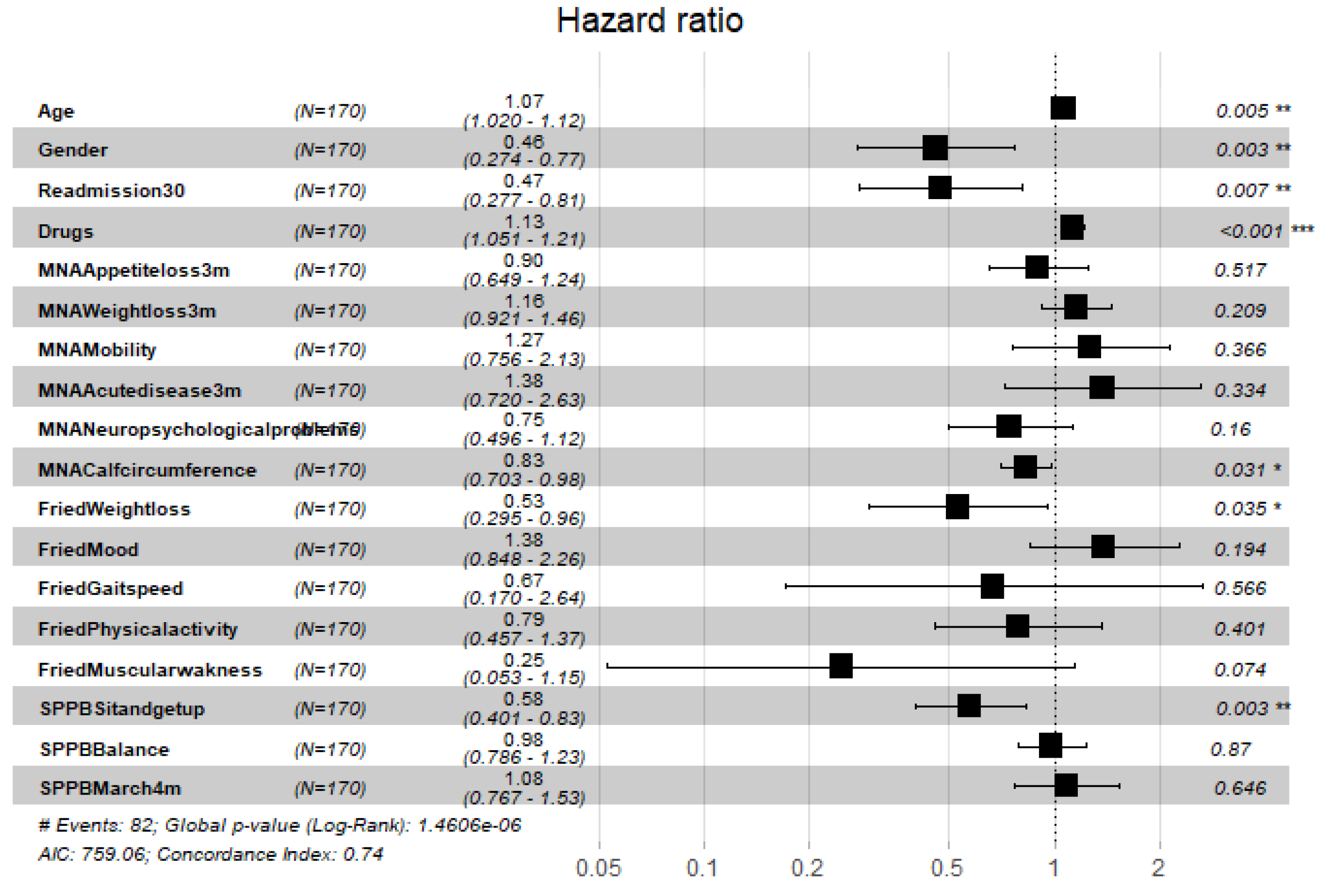
	1 month	6 months	1 year	2 years
Variable	HR (95%CI)	HR (95%CI)	HR (95%CI)	HR (95%CI)
Age	1.05 (1.00,1.09)	1.04 (1.00,1.09)	1.05 (1.00,1.10)	1.05 (1.00,1.10)
Gender	0.63 (0.38,1.02)	0.52 (0.31,0.86)	0.48 (0.28,0.80)	0.48 (0.28,0.80)
R30	0.65 (0.38,1.11)	0.53 (0.31,0.90)	0.53 (0.30,0.89)	0.52 (0.30,0.89)
ND	1.08 (1.01,1.15)	1.10 (1.03,1.18)	1.13 (1.05,1.21)	1.13 (1.05,1.21)
MNA-SF-CC	0.90 (0.76,1.06)	0.85 (0.72,1.00)	0.83 (0.70,0.98)	0.83 (0.70,0.98)
FFI-WL	0.55 (0.30,0.99)	0.59 (0.32,1.05)	0.50 (0.27,0.90)	0.53 (0.29,0.94)
SPPB-SUG	0.72 (0.504,01.02)	0.68 (0.47,0.98)	0.65 (0.45,0.94)	0.64 (0.44,0.92)
Falls	1.65 (0.98,2.74)	1.53 (0.91,2.56)	1.46 (0.87,2.46)	1.40 (0.83,2.35)
Cholesterol	1.55 (0.91,2.61)	1.61 (0.95,2.72)	1.63 (0.96,2.76)	1.52 (0.89,2.57)
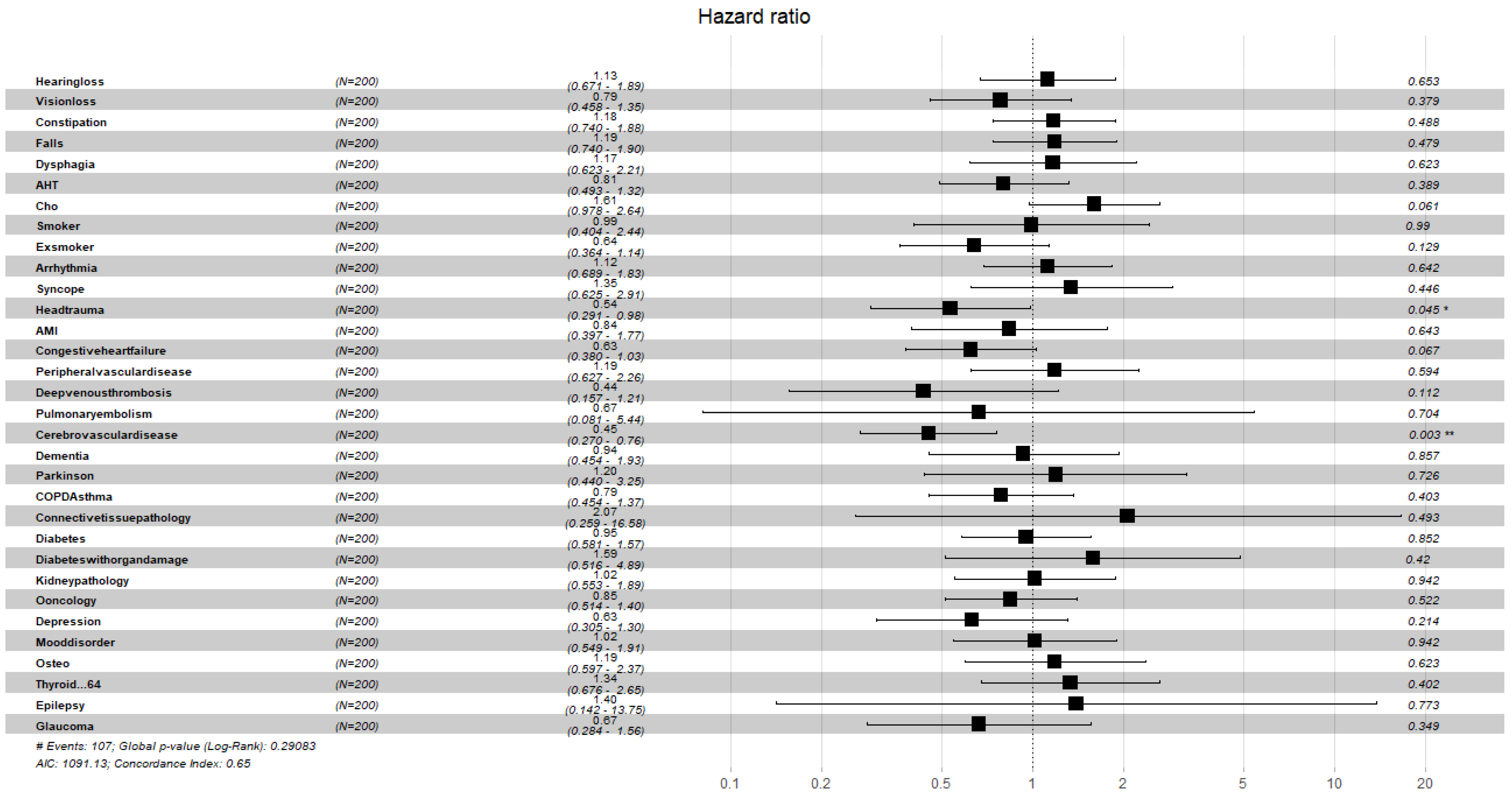
Head Trauma	0.51 (0.262,1.00)	0.54 (0.28,1.07)	0.53 (0.26,1.06)	0.54 (0.27,1.06)
CD	0.49 (0.27,0.87)	0.47 (0.26,0.84)	0.48 (0.26,0.87)	0.52 (0.28,0.96)
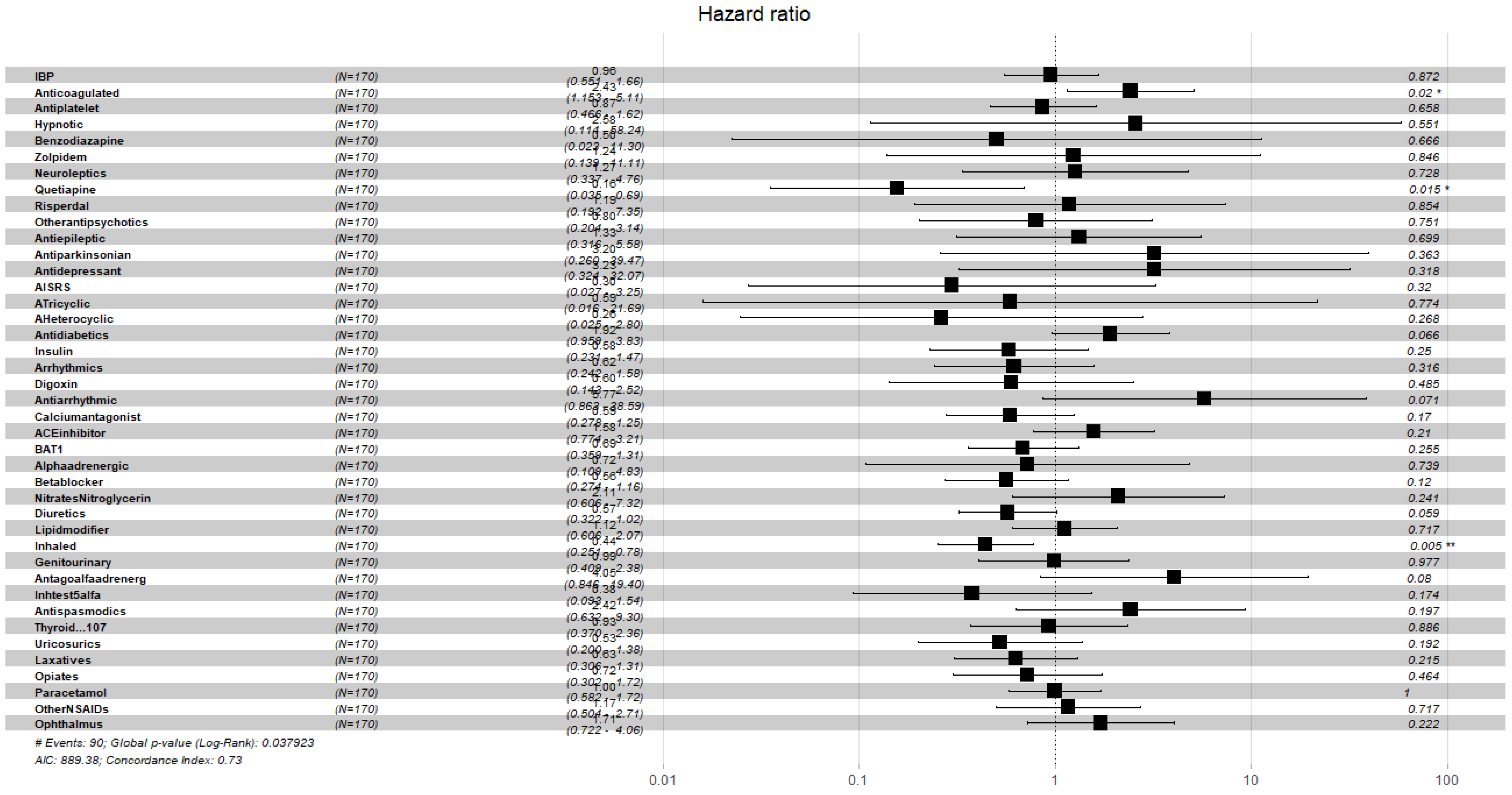
Anticoagulated	1.74 (0.85,3.54)	2.11 (1.01,4.38)	2.37 (1.12,4.98)	2.43 (1.15,5.11)
Quetiapine	0.23 (0.05,0.93)	0.16 (0.03,0.67)	0.15 (0.03,0.66)	0.16 (0.03,0.69)
Diuretics	0.61 (0.34,1.08)	0.58 (0.32,1.03)	0.60 (0.33,1.06)	0.57 (0.32,1.02)
IB	0.51 (0.29,0.87)	0.43 (0.24,0.75)	0.43 (0.24,0.75)	0.44 (0.25,0.78)

Note: HR(95% CI)—mean hazard risk (95% confidence interval). HR significant = p < 0.05. Nonsignificant variables were excluded from the table. Prevalent cohort: patients admitted with delirium (N = 170); gender—0 if male; R30—0 if patient experienced readmission in the 30 days after discharge; ND—number of drugs in polypharmacy; FFI—Fried Frailty Index; FFI-WL—weight loss from the FFI test; SPPB-SUG—sit and stand up from the SPPB test; MNA-CC—calf circumference from the MNA-SF evaluation. Falls—number of fall events in the previous month; Head Trauma—0 if there was head trauma at admission; CD—0 if there was history of cerebrovascular disease; Anticoagulated—use of any anticoagulation drug; quetiapine = 0 if there was use of quetiapine; Diuretics—use of any diuretic drug; IB = 0 if there was use of inhaled bronchodilators.

and

Table 6. Summary of variables with significant hazard risk found by Cox’s regression carried out over families of variables for the incident cohort, data censored after 1 month, 6 months, 1 year, and 2 years.

	1 month	6 months	1 year	2 years
Variable	HR (95%CI)	HR (95%CI)	HR (95%CI)	HR (95%CI)
Age	1.05 (1.00,1.1)	1.05 (1.01,1.10)	1.06 (1.01,1.11)	1.07 (1.02,1.11)
Gender	0.65 (0.42,1.0)	0.48 (0.30,0.75)	0.43 (0.26,0.69)	0.43 (0.26,0.69)
R30	0.62 (0.39,1.0)	0.51 (0.32,0.83)	0.51 (0.31,0.81)	0.50 (0.30,0.80)
ND	1.07 (1.00,1.14)	1.08 (1.02,1.15)	1.10 (1.03,1.17)	1.10 (1.03,1.18)
FFI	1.72 (0.92,3.2)	1.82 (0.98,3.41)	1.83 (0.98,3.41)	1.81 (0.97,3.36)
FFI-WL	0.50 (0.30,0.83)	0.51 (0.31,0.84)	0.42 (0.25,0.70)	0.45 (0.26,0.74)
SPPB-SGU	0.74 (0.55,1.01)	0.71 (0.52,0.97)	0.68 (0.50,0.93)	0.67 (0.49,0.92)
Cholesterol	1.62 (0.99,2.64)	1.68 (1.03,2.76)	1.70 (1.03,2.80)	1.61 (0.97,2.64)
Head Trauma	0.54 (0.29,0.99)	0.56 (0.30,1.03)	0.56 (0.30,1.04)	0.54 (0.29,0.98)
CD	0.47 (0.29,0.77)	0.44 (0.26,0.72)	0.44 (0.26,0.73)	0.45 (0.27,0.76)
Diuretics	0.58 (0.35,0.97)	0.59 (0.34,0.98)	0.59 (0.35,0.99)	0.57 (0.34,0.96)
$\alpha$-Adrenergic Antagonist	2.68 (0.74,9.65)	3.69 (0.98,13.78)	3.92 (1.07,14.37)	4.17 (1.09,15.87)
$5\alpha$ Testosterone inhibitors	0.36 (0.11,1.18)	0.31 (0.09,1.04)	0.28 (0.08,0.94)	0.28 (0.08,0.94)

Note: HR(95% CI)—mean hazard risk (95% confidence interval). HR significant when p < 0.05. Nonsignificant variables were excluded from the table. Incident cohort: patients admitted with delirium or that experienced delirium during hospital stay (N = 200). Gender—0 if male; R30—0 if patient experienced readmission in the 30 days after discharge; ND = number of drugs in polypharmacy; FFI—Fried Frailty Index; FFI-WL—weight loss from the FFI test; SPPB-SUG—sit and stand up from the SPPB test. Head Trauma—0 if there was head trauma at admission; CD—0 if there was history of cerebrovascular disease; Diuretics—use of any diuretic drug; α-Adrenergic Antagonist—number of α-adrenergic antagonist drugs; 5α Testosterone inhibitors—0 use of 5α testosterone inhibitors.

contain the variables with significant HR for the prevalent and incident cohorts, respectively, at considered censoring times. High HR variables identified in both delirium cohorts at some censoring times were age, gender (male), the number of drugs, the occurrence of readmissions before 30 days after discharge, FFI weight loss, SPPB time to sit and stand up, cholesterol (dyslipidemia), head trauma, cerebrovascular disease, and the use of diuretics was high. Specific HRs in the prevalent cohort were anticoagulated, quetiapine, and inhaled bronchodilators. Specific HRs in the incident cohort were $\alpha$-adrenergic antagonist and $5\alpha$ testosterone inhibitors, which were additional risk factors. Specifically, variables with the most significant 2-year hazard risks (HR(95%CI)) for patients with delirium were the following: male gender (0.43 (0.26,0.69)), weight loss (0.45 (0.26,0.74)), sit and stand up test (0.67 (0.49,0.92)), readmission in 30 days after discharge (0.50 (0.30,0.80)), cerebrovascular disease (0.45 (0.27,0.76)), head trauma (0.54 (0.29,0.98)), number of prescribed drugs (polypharmacy) (1.10 (1.03,1.18)), and the use of diuretics (0.57 (0.34,0.96)).

4. Discussion

The sample contained very old patients that were living in the community, in their own houses (71.52%), and some living alone (26.31%); thus, their basal (1 month before hospital admission) performance in the activities of daily living (ADL) was high, and most (89.00%) were either fully independent or had low-level dependency. However, at hospital admission, most patients were frail (69% scored FFI above three, 64% scored SPPB below three). Moreover, 17% had malnutrition and 47% were at risk of malnutrition, similar to [54]. The average Charlson comorbidity index of the sample was 6.39, which corresponded to less than a 2% 10-year survival probability [55]. Their admittance was due to infectious causes, exacerbations of heart failure, and delirium. Infectious causes for admittance are becoming prevalent in the ageing population, amounting to one-third of death causes in people older than 65 years [56].

Both frailty and delirium are associated with vulnerability and a lack of physiologic and cognitive reserve against insults [20,57]. Consequently, delirium HRs are strongly related to the frailty status of the subjects, with specific HRs being age, polypharmacy, hospital readmission, low scores in the sit and stand up test, weight loss, head trauma, cerebrovascular disease, dyslipidemia, and the use of diuretics. Dyslipidemia is a high risk factor [58] for cerebrovascular disease, which was ranked second among the main causes of death by the WHO in 2019 (https://www.who.int/es/news-room/fact-sheets/detail/the-top-10-causes-of-death, accessed on 1 February 2022).

A recent meta-analysis reported that the lower resistance in the sit and get up test, a smaller calf circumference, and weight loss are quite significant frailty risk factors [59]. Weight loss is often the last of the five characteristics of the Fried frailty phenotype to manifest, and it is extremely difficult to revert [60]; hence, it increases delirium mortality. The strength of the lower limbs measured by the sit and stand up test is a biomarker of disease severity [61] that is partly due to malnutrition and a lack of exercise [62]. These factors contribute to ageing adverse events, such as falls, which can produce head trauma that increases mortality in older patients with anticoagulant pharmacy [63], a known risk for older people [64]. Readmission before 30 days of discharge should be considered as another frailty indicator, but has not often been recognized as such.

Ageing is associated with physiological changes that affect drug pharmacokinetics and pharmacodynamics. This study found that increasing the number of drugs was a significant hazard risk for mortality, in agreement with recent findings [65,66,67,68,69,70,71,72,73,74,75]. Dehydration and acute kidney injury are well-know precipitating factors for delirium [1,2,3,9]; therefore, it is not surprising that diuretics were a highly significant hazard risk, because they are widely used as treatments of common diseases: arterial hypertension, heart failure, and renal disease. Electrolyte disturbances cause most side effects, such as delirium, raising concerns regarding diuretics overuse [76]. In the prevalent cohort, the study found inhaled bronchodilators, which have a known effect on the generation of heart arrhythmias [77], and quetiapine, which is an antipsychotic medicament used for patients whose neuropsychiatric symptoms have not responded to other alternative pharma. This finding was in agreement with literature reporting that quetiapine increases mortality by 2% [78]. However, recent publications propose low-dose quetiapine for delirium prevention in critically ill patients [79]. Here, its use could be interpreted as an indicator that delirium overlaps with dementia for some patients, as often found in the literature [14]. However, dementia was not found to be a significant hazard risk for mortality after delirium in this study. In the incident cohort, we found that urology indicated medicaments, such as $\alpha$-adrenergic antagonist and $5\alpha$ testosterone inhibitors, usually treating symptoms associated with benign prostatic hyperplasia. This finding was closely related with the higher mortality risk for males.

Limitations

The identification of mortality risk factors associated with delirium in a cohort was heavily dependent on its demographics and prevalent conditions. Another limitation was that the cohort was recruited in a single site. We did not separately analyse the core symptoms of delirium that could provide additional insights [39]. It was not possible to evaluate recuperation from delirium after hospital discharge [12]. At hospital discharge, it was not feasible to repeat the physical and cognitive assessments due to discharge procedures. There was a lack of detailed records on the duration of the delirium, which could be a target for further research. The management of delirious patients is very delicate, so that the patient assessment and the realization of the physical and cognitive tests may lead to an unintended estimation bias in the evaluation of their hazard risks. The information extracted from the EHR, such as pharmacological data, should not produce any specific estimation bias.

5. Conclusions and Future Work

The objectives of the present study were two-fold: firstly, the assessment of an increased mortality due to delirium in an already frail population; secondly, the identification of high-risk variables. A comparison of the survival probability curves confirmed that delirium was a factor for greater mortality at the four censoring times considered. The findings of the study, in decreasing order of hazard risk significance, were the frailty indices, polypharmacy, the use of diuretics, and some comorbidities associated with delirium onset, such as high cholesterol, cerebrovascular disease, and head trauma.

References

- Setters, B.; Solberg, L.M. Delirium. Prim Care 2017, 44, 541–559. [Google Scholar] [CrossRef] [PubMed]
- Inouye, S.K.; Westendorp, R.G.J.; Saczynski, J.S. Delirium in elderly people. Lancet 2014, 383, 911–922. [Google Scholar] [CrossRef] [Green Version]
- Wilson, J.E.; Mart, M.F.; Cunningham, C.; Shehabi, Y.; Girard, T.D.; MacLullich, A.M.J.; Slooter, A.J.C.; Ely, E.W. Delirium. Nat. Rev. Dis. Prim. 2020, 6, 90. [Google Scholar] [CrossRef]
- Hshieh, T.T.; Inouye, S.K.; Oh, E.S. Delirium in the Elderly. Clin. Geriatr. Med. 2020, 36, 183–199. [Google Scholar] [CrossRef] [PubMed]
- Czok, M.; Pluta, M.P.; Putowski, Z.; Krzych, Ł.J. Postoperative Neurocognitive Disorders in Cardiac Surgery: Investigating the Role of Intraoperative Hypotension. A Systematic Review. Int. J. Environ. Res. Public Health 2021, 18, 786. [Google Scholar] [CrossRef] [PubMed]
- Kang, T.; Park, S.Y.; Lee, J.H.; Lee, S.H.; Park, J.H.; Kim, S.K.; Suh, S.W. Incidence & Risk Factors of Postoperative Delirium After Spinal Surgery in Older Patients. Sci. Rep. 2020, 10, 9232. [Google Scholar] [CrossRef] [PubMed]
- Jung, P.; Pereira, M.A.; Hiebert, B.; Song, X.; Rockwood, K.; Tangri, N.; Arora, R.C. The impact of frailty on postoperative delirium in cardiac surgery patients. J. Thorac. Cardiovasc. Surg. 2015, 149, 869–875. [Google Scholar] [CrossRef] [PubMed] [Green Version]
- Lipowski, Z.J. Delirium (acute confusional states). JAMA 1987, 258, 1789–1792. [Google Scholar] [CrossRef]
- Magny, E.; Le Petitcorps, H.; Pociumban, M.; Bouksani-Kacher, Z.; Pautas, É.; Belmin, J.; Bastuji-Garin, S.; Lafuente-Lafuente, C. Predisposing and precipitating factors for delirium in community-dwelling older adults admitted to hospital with this condition: A prospective case series. PLoS ONE 2018, 13, e0193034. [Google Scholar] [CrossRef]
- Cano-Escalera, G.; Graña, M.; Irazusta, J.; Labayen, I.; Besga, A. Risk factors for prediction of delirium at hospital admittance. Expert Syst. 2021, e12698. [Google Scholar] [CrossRef]
- Ocagli, H.; Bottigliengo, D.; Lorenzoni, G.; Azzolina, D.; Acar, A.S.; Sorgato, S.; Stivanello, L.; Degan, M.; Gregori, D. A Machine Learning Approach for Investigating Delirium as a Multifactorial Syndrome. Int. J. Environ. Res. Public Health 2021, 18, 7105. [Google Scholar] [CrossRef] [PubMed]
- Cole, M.G.; Bailey, R.; Bonnycastle, M.; McCusker, J.; Fung, S.; Ciampi, A.; Belzile, E.; Bai, C. Partial and No Recovery from Delirium in Older Hospitalized Adults: Frequency and Baseline Risk Factors. J. Am. Geriatr. Soc. 2015, 63, 2340–2348. [Google Scholar] [CrossRef]
- Morandi, A.; Davis, D.; Fick, D.M.; Turco, R.; Boustani, M.; Lucchi, E.; Guerini, F.; Morghen, S.; Torpilliesi, T.; Gentile, S.; et al. Delirium superimposed on dementia strongly predicts worse outcomes in older rehabilitation inpatients. J. Am. Med. Dir. Assoc. 2014, 15, 349–354. [Google Scholar] [CrossRef] [PubMed]
- Fong, T.G.; Davis, D.; Growdon, M.E.; Albuquerque, A.; Inouye, S.K. The interface between delirium and dementia in elderly adults. Lancet Neurol. 2015, 14, 823–832. [Google Scholar] [CrossRef] [Green Version]
- Chung, H.Y.; Wickel, J.; Brunkhorst, F.M.; Geis, C. Sepsis-Associated Encephalopathy: From Delirium to Dementia? J. Clin. Med. 2020, 9, 703. [Google Scholar] [CrossRef] [Green Version]
- Clegg, A.; Young, J.; Iliffe, S.; Rikkert, M.O.; Rockwood, K. Frailty in elderly people. Lancet 2013, 381, 752–762. [Google Scholar] [CrossRef] [Green Version]
- Fried, L.; Tangen, C.; Walston, J.; Newman, A.; Hirsch, C.; Gottdiener, J.; Seeman, T.; Tracy, R.; Kop, W.; Burke, G.; et al. Frailty in older adults: Evidence for a phenotype. J. Gerontol. A Biol. Sci. Med. Sci. 2001, 56, M146–M156. [Google Scholar] [CrossRef]
- Rodriguez-Mañas, L.; Fried, L.P. Frailty in the clinical scenario. Lancet 2015, 385, e7–e9. [Google Scholar] [CrossRef]
- Besga, A.; Ayerdi, B.; Alcalde, G.; Manzano, A.; Lopetegui, P.; Graña, M.; González-Pinto, A. Risk Factors for Emergency Department Short Time Readmission in Stratified Population. BioMed Res. Int. 2015, 2015, 685067. [Google Scholar] [CrossRef] [Green Version]
- Verloo, H.; Goulet, C.; Morin, D.; von Gunten, A. Association between frailty and delirium in older adult patients discharged from hospital. Clin. Interv. Aging 2016, 11, 55–63. [Google Scholar] [CrossRef] [Green Version]
- Joosten, E.; Demuynck, M.; Detroyer, E.; Milisen, K. Prevalence of frailty and its ability to predict in hospital delirium, falls, and 6-month mortality in hospitalized older patients. BMC Geriatr. 2014, 14, 1. [Google Scholar] [CrossRef] [Green Version]
- Chu, C.S.; Liang, C.K.; Chou, M.Y.; Lin, Y.T.; Hsu, C.J.; Chou, P.H.; Chu, C.L. Short-Form Mini Nutritional Assessment as a useful method of predicting the development of postoperative delirium in elderly patients undergoing orthopedic surgery. Gen. Hosp. Psychiatry 2016, 38, 15–20. [Google Scholar] [CrossRef] [PubMed]
- Bellelli, G.; Moresco, R.; Panina-Bordignon, P.; Arosio, B.; Gelfi, C.; Morandi, A.; Cesari, M. Is Delirium the Cognitive Harbinger of Frailty in Older Adults? A Review about the Existing Evidence. Front. Med. 2017, 4, 188. [Google Scholar] [CrossRef] [PubMed] [Green Version]
- Bucht, G.; Gustafson, Y.; Sandberg, O. Epidemiology of delirium. Dement. Geriatr. Cogn. Disord. 1999, 10, 315–318. [Google Scholar] [CrossRef]
- Gibb, K.; Seeley, A.; Quinn, T.; Siddiqi, N.; Shenkin, S.; Rockwood, K.; Davis, D. The consistent burden in published estimates of delirium occurrence in medical inpatients over four decades: A systematic review and meta-analysis study. Age Ageing 2020, 49, 352–360. [Google Scholar] [CrossRef] [Green Version]
- Flaherty, J.H.; Morley, J.E. Delirium in the Nursing Home. J. Am. Med. Dir. Assoc. 2013, 14, 632–634. [Google Scholar] [CrossRef]
- Ohl, I.C.B.; Chavaglia, S.R.R.; Ohl, R.I.B.; Lopes, M.C.B.T.; Campanharo, C.R.V.; Okuno, M.F.P.; Batista, R.E.A. Evaluation of delirium in aged patients assisted at emergency hospital service. Rev. Bras. Enferm. 2019, 72, 153–160. [Google Scholar] [CrossRef] [Green Version]
- Feldman, J.; Yaretzky, A.; Kaizimov, N.; Alterman, P.; Vigder, C. Delirium in an acute geriatric unit: Clinical aspects. Arch. Gerontol. Geriatr. 1999, 28, 37–44. [Google Scholar] [CrossRef]
- Fong, T.G.; Tulebaev, S.R.; Inouye, S.K. Delirium in elderly adults: Diagnosis, prevention and treatment. Nat. Rev. Neurol. 2009, 5, 210–220. [Google Scholar] [CrossRef] [PubMed]
- Nguyen, P.V.Q.; Pelletier, L.; Payot, I.; Latour, J. The Delirium Drug Scale is associated with delirium incidence in the emergency department. Int. Psychogeriatr. 2018, 30, 503–510. [Google Scholar] [CrossRef] [PubMed]
- Zhang, Q.; Li, S.; Chen, M.; Yang, Q.; Cao, X.; Ge, L.; Di, B. Delirium screening tools in the emergency department: A protocol for systematic review and meta-analysis. Medicine 2021, 100, e24779. [Google Scholar] [CrossRef] [PubMed]
- Aung Thein, M.Z.; Pereira, J.V.; Nitchingham, A.; Caplan, G.A. A call to action for delirium research: Meta-analysis and regression of delirium associated mortality. BMC Geriatr. 2020, 20, 325. [Google Scholar] [CrossRef]
- Klein Klouwenberg, P.M.C.; Zaal, I.J.; Spitoni, C.; Ong, D.S.Y.; van der Kooi, A.W.; Bonten, M.J.M.; Slooter, A.J.C.; Cremer, O.L. The attributable mortality of delirium in critically ill patients: Prospective cohort study. BMJ 2014, 349. [Google Scholar] [CrossRef] [PubMed] [Green Version]
- Wolters, A.E.; van Dijk, D.; Pasma, W.; Cremer, O.L.; Looije, M.F.; de Lange, D.W.; Veldhuijzen, D.S.; Slooter, A.J. Long-term outcome of delirium during intensive care unit stay in survivors of critical illness: A prospective cohort study. Crit. Care 2014, 18, R125. [Google Scholar] [CrossRef] [Green Version]
- Sanchez, D.; Brennan, K.; Al Sayfe, M.; Shunker, S.A.; Bogdanoski, T.; Hedges, S.; Hou, Y.C.; Lynch, J.; Hunt, L.; Alexandrou, E.; et al. Frailty, delirium and hospital mortality of older adults admitted to intensive care: The Delirium (Deli) in ICU study. Crit. Care 2020, 24, 609. [Google Scholar] [CrossRef]
- Duprey, M.S.; van den Boogaard, M.; van der Hoeven, J.G.; Pickkers, P.; Briesacher, B.A.; Saczynski, J.S.; Griffith, J.L.; Devlin, J.W. Association between incident delirium and 28- and 90-day mortality in critically ill adults: A secondary analysis. Crit. Care 2020, 24, 161. [Google Scholar] [CrossRef] [PubMed] [Green Version]
- Ely, E.W.; Shintani, A.; Truman, B.; Speroff, T.; Gordon, S.M.; Harrell, F.E., Jr.; Inouye, S.K.; Bernard, G.R.; Dittus, R.S. Delirium as a Predictor of Mortality in Mechanically Ventilated Patients in the Intensive Care Unit. JAMA 2004, 291, 1753–1762. [Google Scholar] [CrossRef] [Green Version]
- Gower, L.E.J.; Gatewood, M.O.; Kang, C.S. Emergency department management of delirium in the elderly. West J. Emerg. Med. 2012, 13, 194–201. [Google Scholar] [CrossRef]
- Diwell, R.A.; Davis, D.H.; Vickerstaff, V.; Sampson, E.L. Key components of the delirium syndrome and mortality: Greater impact of acute change and disorganised thinking in a prospective cohort study. BMC Geriatr. 2018, 18, 24. [Google Scholar] [CrossRef]
- Avelino-Silva, T.J.; Campora, F.; Curiati, J.A.E.; Jacob-Filho, W. Association between delirium superimposed on dementia and mortality in hospitalized older adults: A prospective cohort study. PLoS Med. 2017, 14, e1002264. [Google Scholar] [CrossRef] [Green Version]
- Blodgett, J.M.; Theou, O.; Howlett, S.E.; Rockwood, K. A frailty index from common clinical and laboratory tests predicts increased risk of death across the life course. GeroScience 2017, 39, 447–455. [Google Scholar] [CrossRef] [PubMed] [Green Version]
- Inouye, S.K.; van Dyck, C.H.; Alessi, C.; Balkin, S.; Siegal, A.P.; Horwitz, R.I. Clarifying Confusion: The Confusion Assessment Method. Ann. Intern. Med. 1990, 113, 941–948. [Google Scholar] [CrossRef]
- Graña, M.; Besga, A. Fragility and deliriium data from UHA [Data set]. Zenodo 2021. [Google Scholar] [CrossRef]
- Guralnik, J.M.; Simonsick, E.M.; Ferrucci, L.; Glynn, R.J.; Berkman, L.F.; Blazer, D.G.; Scherr, P.A.; Wallace, R.B. A Short Physical Performance Battery Assessing Lower Extremity Function: Association With Self-Reported Disability and Prediction of Mortality and Nursing Home Admission. J. Gerontol. 1994, 49, M85–M94. [Google Scholar] [CrossRef] [PubMed]
- Mahoney, F.; Barthel, D. Functional Evaluation: The Barthel Index. Md State Med. J. 1965, 14, 61–65. [Google Scholar] [PubMed]
- Vellas, B.; Guigoz, Y.; Garry, P.J.; Nourhashemi, F.; Bennahum, D.; Lauque, S.; Albarede, J.L. The Mini Nutritional Assessment (MNA) and its use in grading the nutritional state of elderly patients. Nutrition 1999, 15, 116–122. [Google Scholar] [CrossRef]
- Kaiser, M.J.; Bauer, J.M.; Ramsch, C.; Uter, W.; Guigoz, Y.; Cederholm, T.; Thomas, D.R.; Anthony, P.; Charlton, K.E.; Maggio, M.; et al. Validation of the Mini Nutritional Assessment short-form (MNA-SF): A practical tool for identification of nutritional status. JNHA J. Nutr. Health Aging 2009, 13, 782. [Google Scholar] [CrossRef] [PubMed]
- Erkinjuntti, T.; Sulkava, R.; Wikström, J.; Autio, L. Short Portable Mental Status Questionnaire as a Screening Test for Dementia and Delirium Among the Elderly. J. Am. Geriatr. Soc. 1987, 35, 412–416. [Google Scholar] [CrossRef]
- Pfeiffer, E. A short portable mental status questionnaire for the assessment of organic brain deficit in elderly patients. J. Am. Geriatr. Soc. 1975, 23, 433–441. [Google Scholar] [CrossRef]
- Barakat, A.; Mittal, A.; Ricketts, D.; Rogers, B.A. Understanding survival analysis: Actuarial life tables and the Kaplan–Meier plot. Br. J. Hosp. Med. 2019, 80, 642–646. [Google Scholar] [CrossRef]
- Rich, J.T.; Neely, J.G.; Paniello, R.C.; Voelker, C.C.J.; Nussenbaum, B.; Wang, E.W. A practical guide to understanding Kaplan–Meier curves. Otolaryngol. Head Neck Surg. 2010, 143, 331–336. [Google Scholar] [CrossRef] [Green Version]
- Everitt, B.; Hothorn, T. A Handbook of Statistical Analyses Using R; CRC Press: Boca Raton, FL, USA, 2010. [Google Scholar]
- Cox, D.R. Regression Models and Life-Tables. J. R. Stat. Soc. Ser. B (Methodol.) 1972, 34, 187–220. [Google Scholar] [CrossRef]
- Harith, S.; Mohamed, R.; Fazimah, N. Hospitalized Geriatric Malnutrition: A Perspective of Prevalence, Identification and Implications to Patient and Healthcare Cost. Health Environ. J. 2013, 4, 55–67. [Google Scholar]
- Charlson, M.E.; Pompei, P.; Ales, K.L.; MacKenzie, C.R. A new method of classifying prognostic comorbidity in longitudinal studies: Development and validation. J. Chronic. Dis. 1987, 40, 373–383. [Google Scholar] [CrossRef]
- Kline, K.A.; Bowdish, D.M.E. Infection in an aging population. Curr. Opin. Microbiol. 2016, 29, 63–67. [Google Scholar] [CrossRef] [PubMed]
- Dani, M.; Owen, L.H.; Jackson, T.A.; Rockwood, K.; Sampson, E.L.; Davis, D. Delirium, Frailty, and Mortality: Interactions in a Prospective Study of Hospitalized Older People. J. Gerontol. Ser. A 2017, 73, 415–418. [Google Scholar] [CrossRef]
- Yaghi, S.; Elkind, M.S. Lipids and Cerebrovascular Disease. Stroke 2015, 46, 3322–3328. [Google Scholar] [CrossRef] [Green Version]
- Vermeiren, S.; Vella-Azzopardi, R.; Beckwée, D.; Habbig, A.K.; Scafoglieri, A.; Jansen, B.; Bautmans, I. Frailty and the Prediction of Negative Health Outcomes: A Meta-Analysis. J. Am. Med. Dir. Assoc. 2016, 17, 1163.e1–1163.e17. [Google Scholar] [CrossRef]
- Dent, E.; Morley, J.E.; Cruz-Jentoft, A.J.; Woodhouse, L.; Rodríguez-Mañas, L.; Fried, L.P.; Woo, J.; Aprahamian, I.; Sanford, A.; Lundy, J.; et al. Physical Frailty: ICFSR International Clinical Practice Guidelines for Identification and Management. J. Nutr. Health Aging 2019, 23, 771–787. [Google Scholar] [CrossRef] [Green Version]
- Maddocks, M.; Kon, S.S.C.; Jones, S.E.; Canavan, J.L.; Nolan, C.M.; Higginson, I.J.; Gao, W.; Polkey, M.I.; Man, W.D.C. Bioelectrical impedance phase angle relates to function, disease severity and prognosis in stable chronic obstructive pulmonary disease. Clin. Nutr. 2015, 34, 1245–1250. [Google Scholar] [CrossRef]
- Oikawa, S.Y.; Holloway, T.M.; Phillips, S.M. The Impact of Step Reduction on Muscle Health in Aging: Protein and Exercise as Countermeasures. Front. Nutr. 2019, 6, 75. [Google Scholar] [CrossRef] [PubMed] [Green Version]
- Pieracci, F.M.; Eachempati, S.R.; Shou, J.; Hydo, L.J.; Barie, P.S. Use of long-term anticoagulation is associated with traumatic intracranial hemorrhage and subsequent mortality in elderly patients hospitalized after falls: Analysis of the New York State Administrative Database. J. Trauma 2007, 63, 519–524. [Google Scholar] [CrossRef] [PubMed]
- Díez-Manglano, J.; Bernabeu-Wittel, M.; Murcia-Zaragoza, J.; Escolano-Fernández, B.; Jarava-Rol, G.; Hernández-Quiles, C.; Oliver, M.; Sanz-Baena, S. Oral anticoagulation in patients with atrial fibrillation and medical non-neoplastic disease in a terminal stage. Intern Emerg. Med. 2017, 12, 53–61. [Google Scholar] [CrossRef] [PubMed]
- Zia, A.; Kamaruzzaman, S.B.; Tan, M.P. The consumption of two or more fall risk-increasing drugs rather than polypharmacy is associated with falls. Geriatr. Gerontol. Int. 2017, 17, 463–470. [Google Scholar] [CrossRef]
- de Vries, M.; Seppala, L.J.; Daams, J.G.; van de Glind, E.M.M.; Masud, T.; van der Velde, N. Fall-Risk-Increasing Drugs: A Systematic Review and Meta-Analysis: I. Cardiovascular Drugs. J. Am. Med. Dir. Assoc. 2018, 19, 371.e1–371.e9. [Google Scholar] [CrossRef] [PubMed] [Green Version]
- Seppala, L.J.; van de Glind, E.M.M.; Daams, J.G.; Ploegmakers, K.J.; de Vries, M.; Wermelink, A.M.A.T.; van der Velde, N. Fall-Risk-Increasing Drugs: A Systematic Review and Meta-analysis: III. Others. J. Am. Med. Dir. Assoc. 2018, 19, 372.e1–372.e8. [Google Scholar] [CrossRef] [Green Version]
- Axmon, A.; Sandberg, M.; Ahlström, G.; Midlöv, P. Fall-risk-increasing drugs and falls requiring health care among older people with intellectual disability in comparison with the general population: A register study. PLoS ONE 2018, 13, e0199218. [Google Scholar] [CrossRef]
- Hajjar, E.R.; Cafiero, A.C.; Hanlon, J.T. Polypharmacy in elderly patients. Am. J. Geriatr. Pharmacother. 2007, 5, 345–351. [Google Scholar] [CrossRef]
- Hart, L.A.; Phelan, E.A.; Yi, J.Y.; Marcum, Z.A.; Gray, S.L. Use of Fall Risk-Increasing Drugs Around a Fall-Related Injury in Older Adults: A Systematic Review. J. Am. Geriatr. Soc. 2020, 68, 1334–1343. [Google Scholar] [CrossRef]
- Rossi, M.I.; Young, A.; Maher, R.; Rodriguez, K.L.; Appelt, C.J.; Perera, S.; Hajjar, E.R.; Hanlon, J.T. Polypharmacy and health beliefs in older outpatients. Am. J. Geriatr. Pharmacother. 2007, 5, 317–323. [Google Scholar] [CrossRef]
- Al-Musawe, L.; Martins, A.P.; Raposo, J.F.; Torre, C. The association between polypharmacy and adverse health consequences in elderly type 2 diabetes mellitus patients; a systematic review and meta-analysis. Diabetes Res. Clin. Pract. 2019, 155, 107804. [Google Scholar] [CrossRef]
- Formica, M.; Politano, P.; Marazzi, F.; Tamagnone, M.; Serra, I.; Marengo, M.; Falconi, D.; Gherzi, M.; Tattoli, F.; Bottaro, C.; et al. Acute Kidney Injury and Chronic Kidney Disease in the Elderly and Polypharmacy. Blood Purif 2018, 46, 332–336. [Google Scholar] [CrossRef] [PubMed]
- Huang, Y.T.; Steptoe, A.; Wei, L.; Zaninotto, P. The impact of high-risk medications on mortality risk among older adults with polypharmacy: Evidence from the English Longitudinal Study of Ageing. BMC Med. 2021, 19, 321. [Google Scholar] [CrossRef] [PubMed]
- Wastesson, J.W.; Morin, L.; Tan, E.C.K.; Johnell, K. An update on the clinical consequences of polypharmacy in older adults: A narrative review. Expert Opin. Drug Saf. 2018, 17, 1185–1196. [Google Scholar] [CrossRef] [PubMed] [Green Version]
- Wehling, M. Morbus diureticus in the elderly: Epidemic overuse of a widely applied group of drugs. J. Am. Med. Dir. Assoc. 2013, 14, 437–442. [Google Scholar] [CrossRef]
- Ribas, C.D. Mortality and β-Agonists, or the Risk of Statistical Inference. Arch. Bronconeumol. 2007, 43, 355–357. [Google Scholar] [CrossRef]
- Schneider, L.S.; Dagerman, K.S.; Insel, P. Risk of death with atypical antipsychotic drug treatment for dementia: Meta-analysis of randomized placebo-controlled trials. JAMA 2005, 294, 1934–1943. [Google Scholar] [CrossRef]
- Kim, Y.; Kim, H.S.; Park, J.S.; Cho, Y.J.; Yoon, H.I.; Lee, S.M.; Lee, J.H.; Lee, C.T.; Lee, Y.J. Efficacy of Low-Dose Prophylactic Quetiapine on Delirium Prevention in Critically Ill Patients: A Prospective, Randomized, Double-Blind, Placebo-Controlled Study. J. Clin. Med. 2020, 9, 69. [Google Scholar] [CrossRef] [Green Version]