Abstract
Accurate predictions of CO2 emissions have important practical significance for determining the best measures for reducing CO2 emissions and accomplishing the target of reaching a carbon peak. Although some existing models have good modeling accuracy, the improvement of model specifications can provide a more accurate grasp of a system’s future and thus help relevant departments develop more effective targeting measures. Therefore, considering the shortcomings of the existing grey Bernoulli model, in this paper, the traditional model is optimized from the perspectives of the accumulation mode and background value optimization, and the novel grey Bernoulli model NFOGBM(1,1,) is constructed. The effectiveness of the model is verified by using CO2 emissions data from seven major industries in Shaanxi Province, China, and future trends are predicted. The conclusions are as follows. First, the new fractional opposite-directional accumulation and optimization methods for background value determination are effective and reasonable, and the prediction performance can be enhanced. Second, the prediction accuracy of the NFOGBM(1,1,) is higher than that of the NGBM(1,1) and FANGBM(1,1). Third, the forecasting results show that under the current conditions, the CO2 emissions generated by the production and supply of electricity and heat are expected to increase by 23.8% by 2030, and the CO2 emissions of the other six examined industries will decline.
1. Introduction
Since the industrial revolution, due to the combustion of fossil fuels such as coal and oil and continuous deforestation, the concentration of CO2 in the atmosphere has increased significantly [1]. In recent years, with the continuous and rapid growth of CO2 emissions, global warming is a real problem that needs to be solved along with the involvement of scientists. The international community has made active efforts to jointly address climate change, formulate important documents, and provide a basic political framework and legal system for action to address climate change. By the end of 2020, more than 40 countries and economies around the world officially announced carbon neutrality targets. China has the second-largest economy globally, and fossil energy consumption and CO2 emissions there continue to grow, accounting for increasing proportions of the global totals. According to the BP Statistical Review of World Energy 2021, China’s CO2 emissions in 2020 were 9899.33 million tons, accounting for 30.7% of the global total and ranking first worldwide. Considering the seriousness of climate change, in September 2020, China proposed goals to reach peak CO2 emissions by 2030 and achieve carbon neutrality by 2060. At the end of 2021, China successively issued new policies and action plans to meet these carbon peak and carbon neutrality objectives, as well as related medium- and long-term goals. Generally, peak carbon refers to CO2 emissions reaching a maximum in a certain year and then entering a declining phase. Carbon neutrality refers to the total CO2 produced by a particular organization or society being absorbed and offset over a period of time by natural and artificial means such as afforestation, ocean absorption, engineering storage, etc., to achieve relatively “zero” CO2 emissions from human activities.
Shaanxi Province is rich in natural resources and ranks among the top provinces in China in terms of coal and oil production, making it an important energy and chemical industrial base in China, but its CO2 emissions have long been high. Under the background of the “double carbon” target, Shaanxi has formulated strict CO2 emissions reduction targets. To achieve these goals, it is necessary to understand the current CO2 emissions situation in Shaanxi, reasonably predict future CO2 emissions and structural characteristics of CO2-emitting industries, and formulate reasonable carbon emission reduction measures. Therefore, the rational prediction of CO2 emissions has become an important research topic in emissions studies of Shaanxi.
At present, many methods are used to predict CO2 emissions, and they can be divided into five categories. The first includes macroeconomic system models. Scholars often analyze and predict CO2 emissions based on macroeconomic operational mechanisms, including input–output models, CGE models, the LEAP model, etc. [2,3,4]. The second category includes system optimization models. By comprehensively considering the effects of social and economic development, resource endowment, energy-saving technology, environmental constraints, and consumption behaviour, future CO2 emissions can be analyzed and predicted, and corresponding models include the IPAC model and the IAMC model [5,6]. The third category includes index decomposition models. The factors that influence CO2 emissions are identified, and the CO2 emissions trend is predicted according to the analysis results, and corresponding models include the Kaya, IPAT, and STIRPAT models [7,8,9]. The fourth category includes artificial intelligence models. With the development of information technology, artificial intelligence methods, including artificial neural networks, support vector machines, limit learning machines, etc., have been used for CO2 emissions prediction [10,11,12]. The fifth category includes grey prediction models. Most of the above models require including the factors that influence CO2 emissions to ensure the effectiveness of the prediction results, but adding variables often increases the time and cost required for data collection, and some data are difficult or even impossible to collect. Grey methods solve this problem and directly model scenarios without considering the effects of other factors, thus requiring limited data to obtain accurate predictions. Therefore, the grey prediction method is widely used for CO2 emissions prediction in different regions, industries, and countries because of its convenient operation, simple modeling process, and high accuracy [13,14,15,16]. In addition, grey models have been widely employed in cases involving electric power [17,18], renewable energy [19], natural gas [20], tight gas [21], air pollution [22], traffic flows [23], industrial development [24], landslides [25], and COVID-19 [26,27].
Grey prediction modeling is the most active and widely explored branch of grey system theory, and it is also a new research direction in mainstream prediction theory [28]. However, the core model GM(1,1) has some shortcomings, such as limited adaptability and unstable performance; therefore, scholars have improved this model from many perspectives. For example, the accumulation method was optimized by adding opposite-direction accumulation, fractional accumulation, and comfortable accumulation to improve modeling performance [29,30,31]. Additionally, the continuity of data sequences was improved by processing the original data [32,33], and the modeling error was reduced by improving the initial values of the model [34]. Moreover, the calculation of background values, such as through deriving background values based on a nonhomogeneous exponential function, has been improved [35], and Simpson’s law was used to optimize background values [36]. To improve the prediction performance of the model, the quantum optimization [37], grey wolf optimization (GWO) [38], particle swarm optimization (PSO) [39], and many other intelligent optimization algorithms have been applied to find the optimal parameters. The structure of a grey model can also be optimized, such as by changing the grey processes in the model and replacing them with binomial, polynomial, or other functions to build a new model [40,41]. As new information is more helpful than old information in trend assessment, prioritizing new information has become a common way to improve the prediction accuracy of grey models. Scholars often use a rolling prediction mechanism with metabolic thought to establish optimization models; this approach can not only prioritize new information but also prolong the prediction period of results [42,43,44]. The rolling prediction mechanism ensures that the modeling data are up to date by continuously adding new prediction data, which effectively improves the modeling result. In addition, the GM(1,1) model can be combined with artificial intelligence and statistical analysis models to improve the overall prediction accuracy [45,46,47].
However, most of the above models are linear, and there are many nonlinear problems in most real-world scenarios. Chen et al. [48] first proposed a new nonlinear Bernoulli model NGBM(1,1) to predict the exchange rates of Taiwan’s main trading partners and achieved good prediction results. The nonlinear grey Bernoulli model, which is also known as the GM(1,1) power model, can produce results that highly fit the cumulative curve of the original sequence by adjusting the weight index , and it has displayed good prediction performance for nonlinear problems. Moreover, when = 2, this model is called the grey Verhulst model, which is ideal for data that plot along an S-shaped curve. Based on the effectiveness of the grey Bernoulli model in yielding accurate predictions for nonlinear problems, many scholars have optimized NGBM(1,1) from different perspectives. For example, Guo et al. [49] combined the principle of self-memory with an optimized nonlinear grey Bernoulli model to overcome a major weakness of the traditional Bernoulli model—its sensitivity to the initial parameter values. Wu et al. [19] applied fractional accumulation to the grey Bernoulli model to construct the FANGBM(1,1) model and predicted renewable energy consumption in China. Şahin [50] introduced seasonal factors based on the FANGBM(1,1) model, proposed the OFANGBM(1,1) model, and predicted power generation and installed capacities in Turkey. Xie et al. [15] adopted a simple form of conformable fractional calculations and established the CCFNGBM(1,1) model to predict CO2 emissions related to fuel combustion. Zheng et al. [20] proposed the CFNHGBM(1,1,K) model based on the moth-flame optimization (MFO) algorithm to predict natural gas production and consumption. Wang and Wang [51] combined the NGBM(1,1) and FPGM(1,1,) models and proposed GFBGM(1,1,), which was used to predict the per capita primary energy consumption of major economies around the world.
Each improvement of the model specifications contributes to a more accurate prediction of the examined system’s future, thus providing more effective reference values for relevant sectors. Therefore, based on the above research and considering the unique background value error of the traditional grey Bernoulli model, a new background value optimization method is proposed in this paper. Moreover, based on a new fractional opposite-directional accumulation operation, a novel grey Bernoulli model NFOGBM(1,1,,) is established. Based on the carbon emission data obtained from the Shaanxi Provincial Statistical Yearbook, it is found that carbon emissions in Shaanxi Province occur mainly in seven major industries: wholesale, retail trade and catering services (WRTCS), petroleum and natural gas extraction (PNGE) transportation, storage, postal and telecommunication services (TSPTS), smelting and pressing of ferrous metals (SPFM), nonmetal minerals mining and dressing (NMMD), coal mining and dressing (CMD), and the production and supply of electric power, steam, and hot water (PSESH). Therefore, this paper uses these seven data sets to verify the validity of the NFOGBM(1,1,,) model, and the CO2 emissions from seven industries from 2020 to 2030 in Shaanxi Province, China, are predicted by using the new model and a metabolic concept. The main contributions are summarized as follows:
- (1)
- Considering the unique background value error in the nonlinear grey Bernoulli model, a new optimization method is proposed to further reduce the background value error and improve the prediction performance of the model.
- (2)
- By combining the new fractional opposite-direction accumulation operation, background value optimization, and the FANGBM(1,1) model, the NFOGBM(1,1,,) model is constructed, and its optimal parameters are determined with the PSO algorithm.
- (3)
- The effectiveness of the NFOGBM(1,1,,) model is verified by using CO2 emissions data from seven major industries in Shaanxi, China. The results show that the model outperforms other methods. Notably, unlike the NGBM(1,1) model, it avoids the insufficient utilization of new information, and overfitting, which limits the FGNOM(1,1) model, is also avoided.
- (4)
- Based on a metabolic concept, the NFOGBM(1,1,,) model is used to predict the CO2 emissions of seven major industries in Shaanxi Province.
The rest of this paper is organized as follows. In Section 2, a new fractional-order opposite-direction accumulation grey Bernoulli model NFOGBM(1,1,,) is proposed. In Section 3, the effectiveness of the NFOGBM(1,1,,) model is verified by using CO2 emissions data from seven major industries in Shaanxi Province, China, and CO2 emissions from 2020 to 2030 are forecasted based on a metabolic concept. The conclusions of the study are given in Section 4.
2. New Fractional Opposite-Direction Accumulation Grey Bernoulli Model NFOGBM(1,1,,)
In this section, the traditional nonlinear grey Bernoulli model NGBM(1,1) [48] and fractional nonlinear grey Bernoulli model FANGBM(1,1) [19] are briefly introduced, and then, a new fractional opposite-direction accumulation operation and a background value optimization method are proposed. Finally, a new fractional opposite-direction accumulation grey Bernoulli model NFOGBM(1,1,,) is constructed.
2.1. NGBM(1,1) and FANGBM(1,1) Models
Definition 1.
Consider a nonnegative sequence , where represents the transpose operation. is called the -order accumulation sequence of the original sequence, and is the -order accumulation generation matrix, , where
where ,is calledr-order accumulation generation operator (r-AGO), andis the background value sequence of the original series, where
Then
is called the fractional-order nonlinear grey Bernoulli model FANGBM(1,1), where is any real number. When, this model is the nonlinear grey Bernoulli model NGBM(1,1). If both sides of Equation (4) are integrated into the interval [k − 1, k], Equation (4) can be rewritten as
where andare the areas enclosed by the functionsand, respectively, and theaxis in the interval [k −1, k]; thus, the corresponding variables can be approximately set as and, and Equation (5) can be rewritten as
Therefore, according to the least squares method, the parameters in the model can be calculated based on the following formula:
where
By solving Equation (4), the corresponding function of the final time of the model can beobtained:
The final reduction value can be calculated according to the fractional subtraction generation operator (r-IAGO):
2.2. New Fractional Opposite-Direction Accumulation Operation
Definition 2.
Consider a nonnegative sequence , where represents the transpose operation. is called the new r-order opposite-direction accumulation sequence of the original sequence, and is the r-order new opposite-direction accumulation generation matrix, , where
where is called the r-order accumulation generation operator (r-NOAGO). Matrix can be expressed as
As shown above, matrix and matrix satisfy . The new opposite-direction subtraction operator (-INOAGO) corresponding to the new opposite-direction accumulation operator is
New information prioritization is an important principle in grey system modeling; that is, the newest data in the original sequence provide the most valuable grey information, and accordingly, compared with old data, we should prioritize new data in the modeling process. The opposite-direction accumulation operation can be used to prioritize new information [29]. Notably, the extrapolation performance of the traditional model is generally poor, and consequently, the prediction accuracy is low. The new opposite-direction accumulation approach solves this problem by fully considering all available information, thus providing high accuracy and practicality.
2.3. Optimization of Background Value
A certain inherent error is associated with the derivation from Equation (5) to Equation (6); that is, functions and are approximately regarded as and , which is unreasonable. Zhou et al. [52] used the following formula to calculate the background value: . This method of setting the background value can reduce the corresponding model error to a large extent. Therefore, in this paper, the background values of the grey Bernoulli model are defined in a related way, as follows.
Definition 3.
Let , the exact value of which has yet to be determined. The functions and are approximated as and , respectively, where
2.4. A New Fractional Opposite-Direction Accumulation Grey Bernoulli Model (NFOGBM(1,1,,))
The novel fractional opposite-direction accumulation operation, optimization approach for background values, and FANGBM(1,1) model are combined to form the novel fractional opposite-direction accumulation grey Bernoulli model NFOGBM(1,1,,), which is defined as follows.
Definition 4.
Consider a nonnegative sequence , where represents the transpose operation. Then, in NFOGBM(1,1,,) is used, where is as shown in Equation (11). By integrating both sides of the equation, we can approximate the resulting expression as
where and are shown in Equation (14). The development coefficient and grey action are given by , according to the least-squares method, where
The time response equation of the model is , and the final reduced equation is calculated according to Equation (13).
Based on the definition above, the relationship between the NFOGBM(1,1,,) model and other existing grey models can be assessed.
When , , and , the model becomes the traditional GM(1,1) model [28].
When , r = 1, and , the model becomes the grey Verhulst model [21].
When , , and , the model becomes the NGBM(1,1) model [48].
When and is determined as shown in Equation (1), the model becomes the FANGBM(1,1) model [19].
According to Definition 4, the NFOGBM(1,1,,) model has a total of six unknown parameters, among which the development coefficient and grey action are known, but determining the optimal values of the parameters remains a challenge. Therefore, in this paper, the PSO algorithm is used to set these four unknown parameters and minimize the mean relative percent error of simulations (MRSPE). The specific calculation steps are shown in Figure 1 with the following equations.
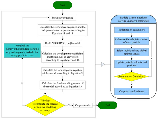
Figure 1.
NFOGBM(1,1,) modeling process.
2.5. Metabolic Ideas and the NFOGBM(1,1,,) Modeling Process
When a grey model is used, the prediction accuracy is often less than ideal when the original data are applied for long-term prediction. Notably, over time, the grey factors that influence the considered variables will continue changing, as will the most recent state of the system. If the original data are used to build the grey prediction model, the prediction accuracy of the model will inevitably decrease, and its reliability will also decrease. Therefore, a grey model can generally only obtain good results when predicting one or two values, and the long-term prediction effect is not satisfactory and can only reflect approximate trends. To remedy this deficiency, a metabolic mechanism needs to be used for modeling.
The so-called metabolic concept involves removing the old data from the original modeling sequence and performing the modeling steps again according to the most recent prediction data generated by the model, i.e., after predicting one or two values, the newly predicted values are added to the original sequence, and the old data in the original genus sequence are removed, thus keeping the dimension of the modeling sequence unchanged. Through such a metabolic concept, new prediction information is continuously added, and the grey level can be gradually reduced until the prediction objectives are met or a certain accuracy requirement is reached.
To clearly demonstrate how the NFOGBM(1,1,,) model proposed in this paper can be used to solve a practical prediction problem, a flowchart is presented in Figure 1.
2.6. Error Metrics
To better verify the reliability and fit of the NFOGBM(1,1,,) model, the mean absolute percentage error (MAPE) is used to assess the accuracy of the model. Given that the test of grey model performance includes simulation performance and prediction performance, the original data need to be divided into modeling and prediction subsets. Each index is then evaluated from simulation, prediction, and overall perspectives. The MAPE of the simulation stage is also called the mean relative percentage error of simulations (MRSPE); the MAPE of the prediction stage is also called the mean prediction percentage error (MRFPE), and the overall MAPE is also known as the combined mean relative percentage error (CMRPE). The MRSPE, MRFPE, and CMRPE are calculated as follows:
where is the number of modeling samples and is the prediction interval.
3. Applications in Forecasting Shaanxi’s CO2 Emissions
In this paper, the data from the seven industries with the highest CO2 emissions in Shaanxi Province are used to verify the prediction performance of the NFOGBM(1,1,,) model, and compare it with the NGBM(1,1) model and FANGBM(1,1) model. On this basis, the CO2 emissions of the seven industries from 2020 to 2030 are predicted to provide a reference for use by relevant departments in Shaanxi Province when formulating carbon reduction policies. The seven industries are WRTCS, PNGE, TSPTS, SPFM, NMMD, CMD, and PSESH. For convenience, the above three models are abbreviated as NFOGBM, FANGBM, and NGBM, respectively. The PSO algorithm is applied to calculate the unknown parameters, and the settings are as follows: learning factors c1 = c2 = 2, the inertia factor is 0.8, the population size is 50, the maximum number of iterations is 300, the range of the cumulative order is [0, 3], and the range of values is [−2, 5].
3.1. Data Description
In this paper, the carbon emission coefficient method is used to measure the CO2 emissions from seven industries in Shaanxi Province, China. The required energy consumption data were obtained from the Shaanxi Provincial Statistical Yearbook, and the carbon emission coefficients and converted standard coal coefficients of various types of energy were based on the IPCC Guidelines for National Greenhouse Gas Inventory and the China Energy Statistical Yearbook. The carbon emissions data for each industry were obtained via calculations, as shown in Table 1 and Figure 2. Among them, WRTCS has the lowest CO2 emissions, with an average of only 4.25 million tons over the past nine years, and PSESH yields the highest CO2 emissions, with its average of 128.6 million tons totalling more than those of the other six sectors combined. In terms of trend, CO2 emissions from four industries, namely, WRTCS, PNGE, TSPTS, and NMMD, have consistently decreased, and CO2 emissions from SPFM have been steadily decreasing since 2014. Additionally, CO2 emissions from CMD have only slightly decreased since 2016. In contrast, the amount of CO2 emitted from PSESH has been increasing at an average annual rate of 4.9%.

Table 1.
CO2 emissions from 7 industries in Shaanxi, 2011–2019 (million tons).
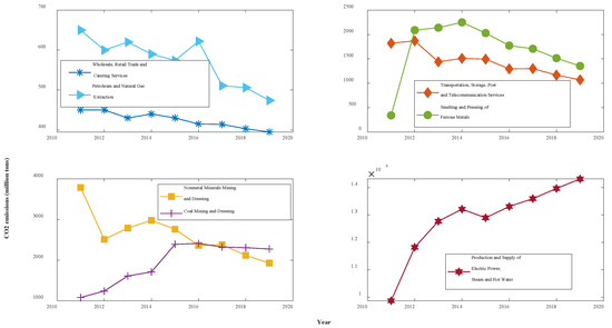
Figure 2.
Trends of CO2 emissions for 7 industries in Shaanxi, 2011–2019.
3.2. Model Comparison
Carbon emissions data from seven industries are analyzed and compared using three models, NFOGBM, FANGBM, and NGBM, to predict data for two years, 2018 and 2019. Then, the simulation, prediction, and overall performance of the three models are assessed.
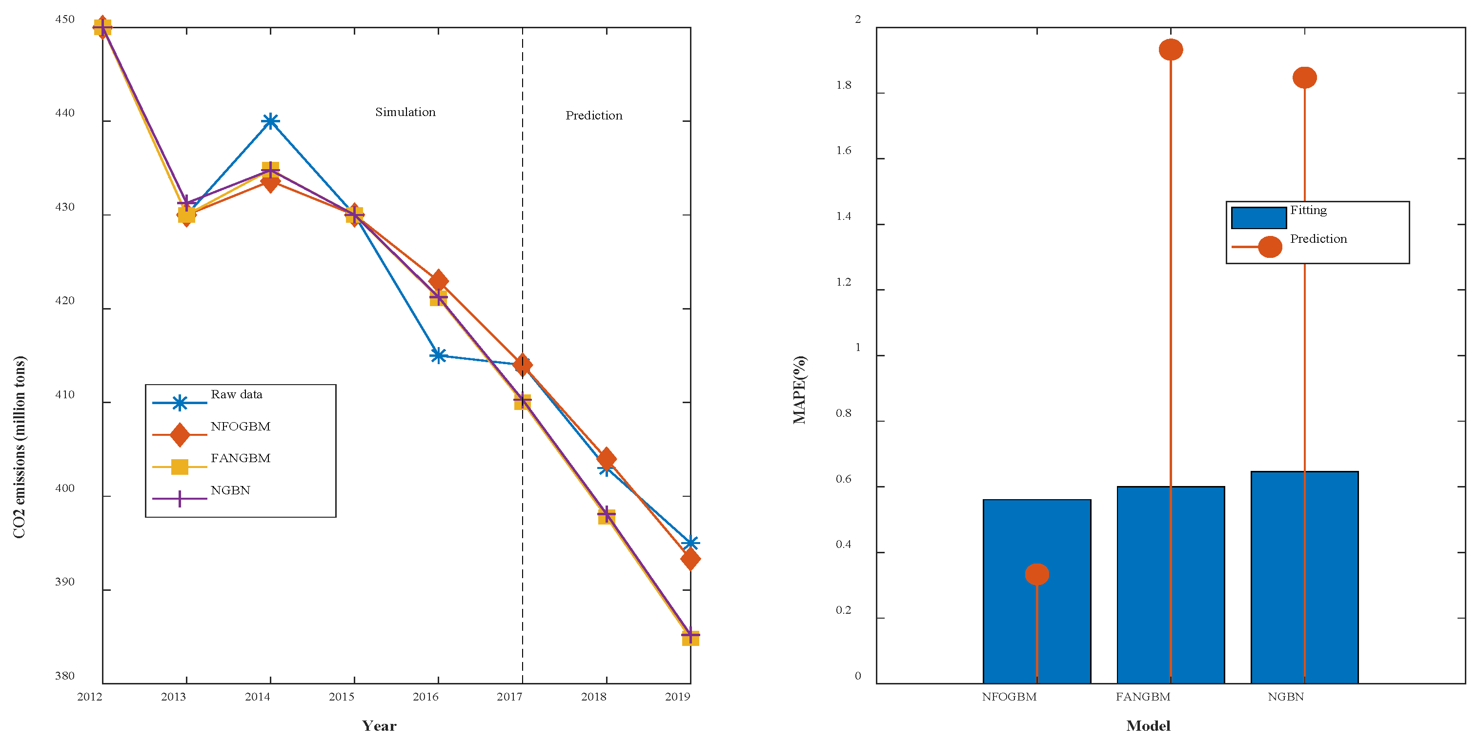
(1) The modeling results for WRTCS are shown in Table 2, and the fitted curves and error plots are shown in Figure 3. The MRPESs (%) of the NFOGBM, FANGBM, and NGBM are 0.561, 0.6, and 0.647, respectively; the MRFPEs (%) are 0.333, 1.932, and 1.847, respectively, and the CMRPEs (%) are 0.504, 0.933, and 0.947, respectively. It can be seen that the simulation errors of the three models are not very different, but the NFOGBM has a much lower prediction error and integrated error than those of the other two models, indicating that the NFOGBM provides the optimal simulation, prediction, and integrated performance. In addition, the curves obtained with the NFOGBM are closest to the original data, indicating that the model provides the best predictions of future scenarios. It is worth noting that the FANGBM reduces the simulation error to some extent but increases the prediction error compared to the NGBM.
Table 2.
Modeling results for WRTCS.
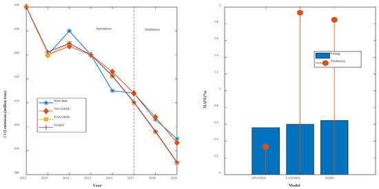
Figure 3.
Fitting curves and error plots of the WRTCS results.
(2) The modeling results for PNGE are shown in Table 3, and the fitting and error plots are shown in Figure 4. The MRPESs (%) of the NFOGBM, FANGBM, and NGBM are 2.498, 2.864, and 3.302, respectively; the MRFPEs (%) are 4.836, 6.222, and 6.415, respectively, and the CMRPEs (%) are 3.084, 3.704, and 4.08, respectively. As in the previous example, the NFOGBM yields the smallest simulation, prediction, and combined errors, and can best capture the trends of the data to produce accurate predictions. It is worth mentioning that the optimal solution of parameter produced by the NFOGBM in this example is 0, implying that .
Table 3.
Modeling results for PNGE.
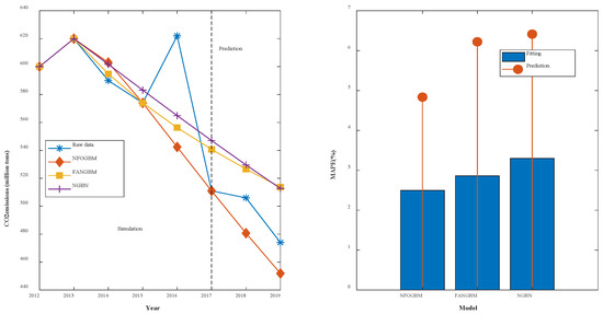
Figure 4.
Fitting curves and error plots of the PNGE results.
(3) The modeling results for TSPTS are shown in Table 4, and the fitting and error plots are shown in Figure 5. The MRPESs (%) of the NFOGBM, FANGBM, and NGBM are 1.52, 1.957, and 2.062, respectively; the MRFPEs (%) are 2.16, 6.244, and 3.806, respectively, and the CMRPEs (%) are 1.68, 3.028, and 2.498, respectively. In this example, the NFOGBM again yields the smallest simulation, prediction, and synthesis errors, and the highest modeling accuracy. Compared to the NGBM, the FANGBM yields some overfitting, which improves the simulation accuracy but leads to low prediction accuracy. Notably, the optimal solution of parameter produced by the NFOGBM in this example is 1, implying that .
Table 4.
Modeling results for TSPTS.

Figure 5.
Fitting curves and error plots of the TSPTS results.
(4) The modeling results for SPFM are shown in Table 5, and the fitting and error diagrams are shown in Figure 6. The MRPESs (%) of the NFOGBM, FANGBM, and NGBM are 1.759, 1.272, and 2.118, respectively; the MRFPEs (%) are 1.837, 5.619, and 3.231, respectively, and the CMRPEs (%) are 1.779, 2.359, and 2.397. In this example, the FANGBM produces the lowest simulation error but has the highest prediction error, resulting in some overfitting, which can be seen in the fitted graphs. The NFOGBM solves this problem, and yields the lowest prediction and synthesis errors as well as the highest modeling accuracy in this example.
Table 5.
Modeling results for SPFM.
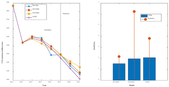
Figure 6.
Fitting curves and error plots of the SPFM results.
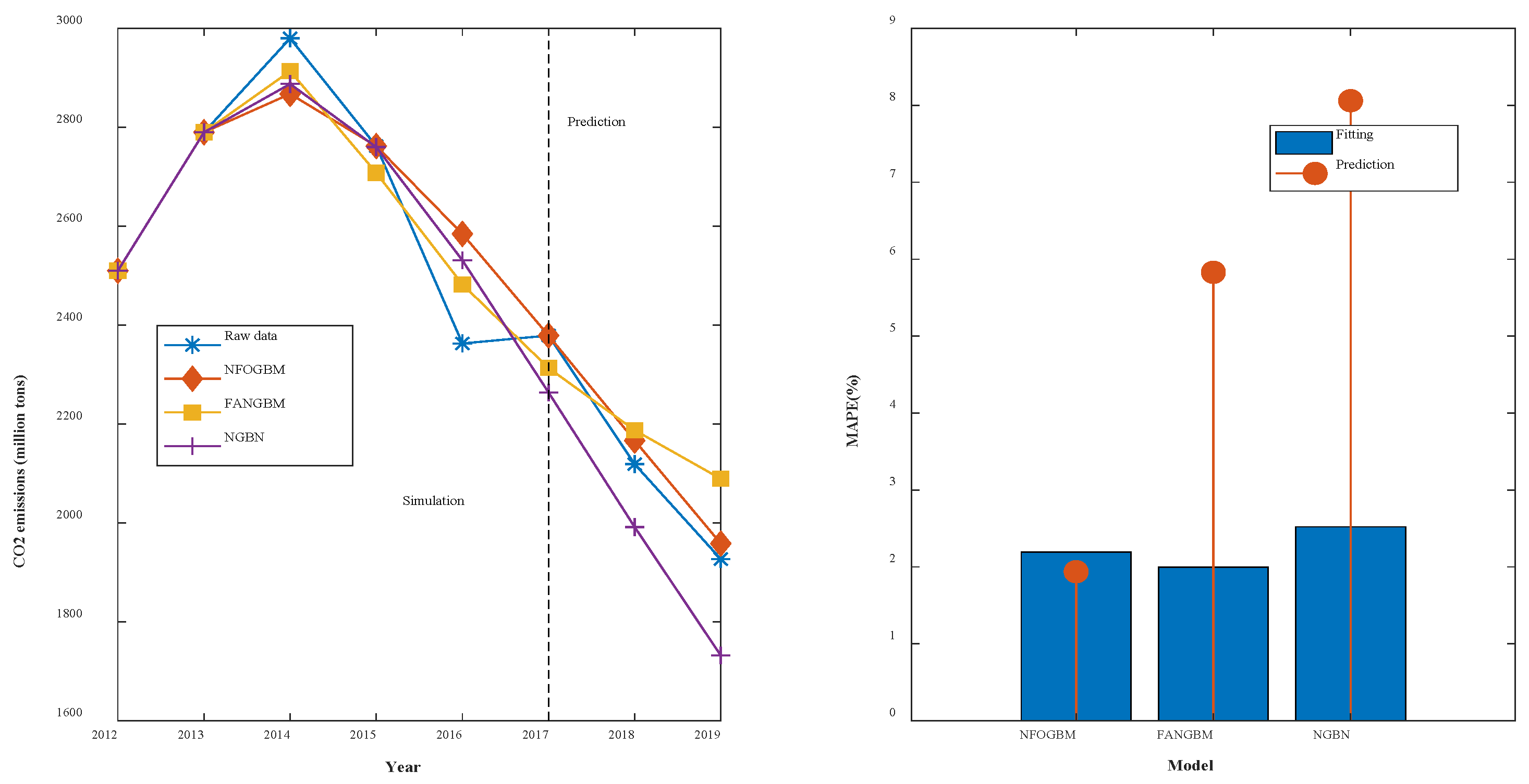
(5) The modeling results for NMMD are shown in Table 6, and the fitting and error plots are shown in Figure 7. The MRPESs (%) of the NFOGBM, FANGBM, and NGBM are 2.191, 1.998, and 2.52, respectively; the MRFPEs (%) are 1.938, 5.83, and 8.06, respectively, and the CMRPEs (%) are 2.128, 2.956, and 3.905. Similar to the previous example, although the FANGBM yields the lowest simulation error, while the NFOGBM produces the lowest prediction error and combined error, and the corresponding modeling curve fits the original data the best; therefore, among these three models, the NFOGBM provides the best modeling accuracy.
Table 6.
Modeling results for NMMD.

Figure 7.
Fitting curves and error plots of the NMMD results.
(6) The modeling results for CMD are shown in Table 7, and the fitting and error plots are shown in Figure 8. The MRPESs (%) of the NFOGBM, FANGBM, and NGBM are 4.112, 3.406, and 4.459, respectively; the MRFPEs (%) are 0.519, 4.104, and 11.146, respectively, and the CMRPEs (%) are 3.727, 4.007, and 6.688, respectively. In this example, the NGBM does not capture the changes in the new data, and the corresponding modeling curve displays an upwards trend in the prediction phase, seriously deviating from the original data. Both the NFOGBM and the FANGBM can use all available information in modeling, and the NFOGBM greatly improves upon the traditional grey Bernoulli model by utilizing new data, yielding the lowest prediction error and comprehensive error, and providing the optimal modeling accuracy.
Table 7.
Modeling results for CMD.
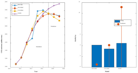
Figure 8.
Fitting curves and error plots of the CMD results.
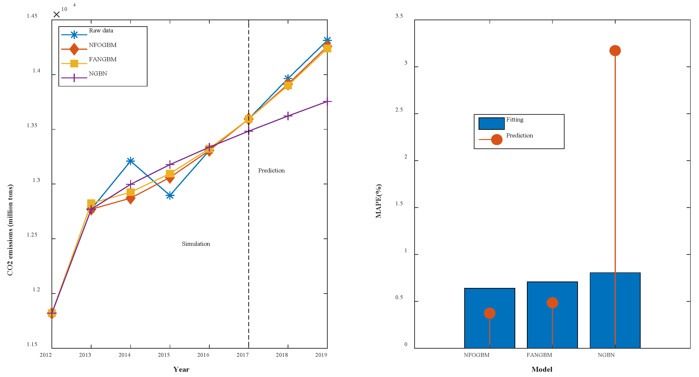
(7) The modeling results for PSESH are shown in Table 8, and the fitting and error plots are shown in Figure 9. The MRPESs (%) of the NFOGBM, FANGBM, and NGBM are 0.64, 0.708, and 0.806, respectively; the MRFPEs (%) are 0.373, 0.485, and 3.172, respectively, and the CMRPEs (%) are 0.573, 0.652, and 1.397, respectively. For the NFOGBM and FANGBM, all three errors are less than 1%, which indicates that these two models perform well for this example. Although the NGBM yields improved simulations in this case compared to those in previous examples, its prediction accuracy is low. Moreover, the NFOGBM yields the lowest simulation, prediction, and synthesis errors, and the highest modeling accuracy, achieving a notable improvement over the traditional grey Bernoulli model.
Table 8.
Modeling results for PSESH.

Figure 9.
Fitting curves and error plots of the PSESH results.
In summary, the FANGBM improves the modeling performance of the NGBM in some cases, but overfitting problems occur in some cases, while the NFOGBM yields low errors, high prediction performance, and the best modeling accuracy in all seven examples because the new background value optimization approach can further reduce the errors in the modeling process and improve the modeling accuracy. The opposite-direction cumulative operation can further enhance the ability of the model to utilize new information, can use grey information to capture the latest change trends in the system, and can also solve the overfitting problem existing in the FANGBM. Thus, the improved grey Bernoulli model based on these two approaches can effectively use the latest data to produce both accurate prediction results that capture the trends of the new data as well as results that are highly compatible with the original data. Thus, the proposed opposite-directional cumulative operation and background value optimization method are reasonable and effective, and the new information prioritization concept can further improve modeling performance.
3.3. Forecasting and Analysis
According to the model results for the seven groups of data above, the NFOGBM yields the highest modeling accuracy among the models considered. Thus, the NFOGBM was applied and combined with a metabolic concept to forecast the CO2 emissions of the seven industries from 2020 to 2030. We first modeled and forecasted the data for 2020 using six datasets from 2014–2019, and then eliminated the old data from 2014 to add the newly predicted 2020 data. This process was then repeated for 2021–2030. The forecasting results are shown in Table 9 and Figure 10.
Table 9.
Forecasted CO2 emissions of 7 industries in Shaanxi (million tons).
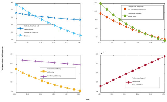
Figure 10.
CO2 emissions curves for the next 11 years in Shaanxi.
The forecasting results show that under the various grey conditions in effect, CO2 emissions are projected to decline in all six sectors—WRTCS, PNGE, TSPTS, SPFM, NMMD, and CMD—and to further increase in the PSESH sector. CO2 emissions in WRTCS are projected to decline at an average rate of 1.3% per year and are projected to decline by 55.5 million tons. CO2 emissions in PNGE are projected to decline at an average rate of 4.6% per year and are expected to decline by 2.39 million tons by 2030. CO2 emissions in TSPTS are projected to decline at an average rate of 5.9% per year and are expected to decline by 6.99 million tons by 2030. CO2 emissions in SPFM are projected to decline at an average rate of 6.8% per year and are expected to decline by 10.19 million tons by 2030. CO2 emissions in NMMD are projected to decline at an average rate of 6.3% per year and are expected to decline by 13.35 million tons by 2030. CO2 emissions in CMD are projected to decline at an average rate of 1.2% per year and are expected to decline by 2.92 million tons by 2030. CO2 emissions in PSESH are projected to increase at an average rate of 2.3% per year and are expected to rise by 25.52 million tons by 2030. For the seven industries combined, as shown in Figure 11, the total CO2 emissions curve shows a convex shape with little overall change, with the value expected to decline by 0.4% by 2030.
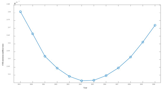
Figure 11.
Overall CO2 emissions curve for Shaanxi Province over the next 11 years.
From the forecast results, four industries, PNGE, TSPTS, SPFM, and NMMD, show a larger proportional CO2 emissions decrease, with emissions expected to drop by more than 50% by 2030. This situation will undoubtedly contribute significantly to the accomplishment of CO2 emissions reduction and carbon neutrality targets, but it is not consistent with the actual situation in Shaanxi Province, where the pace of CO2 emissions reduction is too fast. The excessively fast reduction of CO2 emissions may be due to technological improvements and the further use of clean energy, but the possibility that it is caused by the reduction of energy use by industry, i.e., industry reducing emissions for the sake of reducing emissions, cannot be excluded, and this approach is contradictory to the overall goal of improving people’s economic well-being. Enterprises should steadily reduce their CO2 emissions by using clean energy or upgrading technology while ensuring the normal development of the industry. The government should appropriately reduce the CO2 emissions reduction targets for these four industries to ensure the healthy development of enterprises. The decline in CO2 emissions in WRTCS and CMD is more normal, indicating that the existing policies of enterprises and the government are more applicable to these sectors, and should continue to be implemented.
Considering the overall CO2 emissions of the seven industries, the curve shows a trend of decreasing and then increasing because the increase in CO2 emissions from PSESH in the later period exceeds the decrease in CO2 emissions from other industries. Obviously, the most serious CO2 emissions problem among the seven industries is found in PSESH, which contributes more than half of the total CO2 emissions of the seven industries and still maintains an increasing state. With the continuous improvement of the economic level and the improvement of people’s living standards, the demand for electricity and heat increases, which is inevitable. How to maintain or even reduce the CO2 emissions level while maintaining the normal supply of electricity and heat is a challenge. Enterprises should further improve the use of clean energy and technology to ensure production, and the government should further increase the control of CO2 emissions in the PSESH industry to enforce pressure. Notably, this paper verifies the validity of the NFOGBM(1,1,,) model, which can be applied to the prediction of economic and social fields except CO2 emissions prediction.
4. Conclusions
In this paper, a novel fractional-order inverse cumulative operation method and background value optimization method are proposed, and a new grey model NFOGBM(1,1) is combined with the fractional-order nonlinear Bernoulli model FANGBM(1,1). Then, the validity of the NFOGBM(1,1,,) model is verified using carbon emission data from seven major industries in Shaanxi Province, China. Next, using NFOGBM(1,1,,) and a metabolic concept, the CO2 emissions of the seven industries from 2020 to 2030 are predicted. The following conclusions are obtained. First, the new background value optimization approach is effective and reasonable, and it can improve the performance of the traditional model to achieve accurate prediction. Second, the combination of the new opposite-direction cumulative optimization approach with the traditional grey Bernoulli model is effective, and this approach can utilize new information and solve the overfitting problem of the FANGBM(1,1) model. Third, the NGBM(1,1) model does not sufficiently utilize new information, and the FANGBM(1,1) model produces overfitting in some cases. The NFOGBM(1,1,,) model provides better predictions than and outperforms the NGBM(1,1) and FANGBM(1,1) models, notably improving the prediction accuracy of the traditional grey model. Fourth, the prediction results show that under the current conditions, in 2020–2030, the CO2 emissions from the production and supply of electricity and heat will further increase and are expected to reach 17,865,000 tons by 2030. The CO2 emissions of the remaining six examined industries will all decrease. Therefore, to successfully achieve the carbon peak target in Shaanxi Province, the primary problem that needs to be solved is the excessive and rapid growth of CO2 emissions caused by the production and supply of electricity and heat.
Various types of grey models exist, and in this paper, only the new opposite-directional cumulative and background value optimization approach is applied to the traditional grey Bernoulli model. The effect of combining these two optimization methods with other models is not yet known. Moreover, only the CO2 emissions of each industry in Shaanxi Province are predicted, and the corresponding emission problems are discussed; however, solutions to these problems must be further explored in future research.
Author Contributions
Conceptualization, H.W. and Z.Z.; software Z.Z.; validation, H.W.; data curation, Z.Z.; writing—original draft, Z.Z.; writing—review and editing, H.W.; supervision, H.W.; All authors have read and agreed to the published version of the manuscript.
Funding
This research was funded by Social Science Project of Shaanxi (no. 2021D062), the Youth Innovation Team of Shaanxi Universities (no. 21JP044), and the Shaanxi Soft Science Foundation (no. 2022KRM079, no. 2022KRM171).
Data Availability Statement
The datasets of this paper are available from the corresponding author on reasonable request.
Conflicts of Interest
The authors declare no conflict of interest.
References
- Nema, P.; Nema, S.; Roy, P. An overview of global climate changing in current scenario and mitigation action. Renew. Sustain. Energy Rev. 2012, 16, 2329–2336. [Google Scholar] [CrossRef]
- Di Sbroiavacca, N.; Nadal, G.; Lallana, F.; Falzon, J.; Calvin, K. Emissions reduction scenarios in the Argentinean Energy Sector. Energy Econ. 2016, 56, 552–563. [Google Scholar] [CrossRef] [Green Version]
- Shi, Q.; Chen, J.; Shen, L. Driving factors of the changes in the carbon emissions in the Chinese construction industry. J. Clean. Prod. 2017, 166, 615–627. [Google Scholar] [CrossRef]
- Dong, F.; Yu, B.; Hadachin, T.; Dai, Y.; Wang, Y.; Zhang, S.; Long, R. Drivers of carbon emission intensity change in China. Resour. Conserv. Recycl. 2018, 129, 187–201. [Google Scholar] [CrossRef]
- Beek, L.V.; Vuuren, D.; Hajer, M.; Pelzer, P. Anticipating futures through models: The rise of integrated assessment modelling in the climate science-policy interface since 1970. Glob. Environ. Chang. 2020, 65, 102191. [Google Scholar] [CrossRef]
- Jiang, K.J.; He, C.M.; Zhu, S.L.; Xiang, P.P.; Chen, S. Transport scenarios for China and the role of electric vehicles under global 2 °C/1.5 °C targets. Energy Econ. 2021, 103, 105172. [Google Scholar]
- Ma, M.; Cai, W. What drives the carbon mitigation in Chinese commercial building sector? Evidence from decomposing an extended Kaya identity. Sci. Total. Environ. 2018, 634, 884–899. [Google Scholar] [CrossRef]
- Danish; Ozcan, B.; Ulucak, R. An empirical investigation of nuclear energy consumption and carbon dioxide (CO2) emission in India: Bridging IPAT and EKC hypotheses. Nucl. Eng. Technol. 2021, 53, 2056–2065. [Google Scholar] [CrossRef]
- Huang, J.B.; Li, X.H.; Wang, Y.J.; Lei, H.Y. The effect of energy patents on China’s carbon emissions: Evidence from the STIRPAT model. Technol. Forecast. Soc. 2021, 173, 121110. [Google Scholar] [CrossRef]
- Acheampong, A.; Boateng, E.B. Modelling carbon emission intensity: Application of artificial neural network. J. Clean. Prod. 2019, 225, 833–856. [Google Scholar] [CrossRef]
- Wen, L.; Cao, Y. Influencing factors analysis and forecasting of residential energy-related CO2 emissions utilizing optimized support vector machine. J. Clean. Prod. 2020, 250, 119492. [Google Scholar] [CrossRef]
- Sun, W.; Huang, C. Predictions of carbon emission intensity based on factor analysis and an improved extreme learning machine from the perspective of carbon emission efficiency. J. Clean. Prod. 2022, 338, 130414. [Google Scholar] [CrossRef]
- Yan, C.; Wu, L.F.; Liu, L.Y.; Zhang, K. Fractional Hausdorff grey model and its properties. Chaos Soliton. Fract. 2020, 138, 109915. [Google Scholar]
- Wang, Q.; Li, S.; Pisarenko, Z. Modeling carbon emission trajectory of China, US and India. J. Clean. Prod. 2020, 258, 120723. [Google Scholar] [CrossRef]
- Xie, W.; Wu, W.-Z.; Liu, C.; Zhang, T.; Dong, Z. Forecasting fuel combustion-related CO2 emissions by a novel continuous fractional nonlinear grey Bernoulli model with grey wolf optimizer. Environ. Sci. Pollut. Res. 2021, 28, 38128–38144. [Google Scholar] [CrossRef]
- Hu, Y.-C.; Jiang, P.; Tsai, J.-F.; Yu, C.-Y. An Optimized Fractional Grey Prediction Model for Carbon Dioxide Emissions Forecasting. Int. J. Environ. Res. Public Health 2021, 18, 587. [Google Scholar] [CrossRef]
- Ding, S.; Hipel, K.W.; Dang, Y.G. Forecasting China’s electricity consumption using a new grey prediction model. Energy 2018, 149, 314–328. [Google Scholar] [CrossRef]
- Wu, W.-Z.; Pang, H.; Zheng, C.; Xie, W.; Liu, C. Predictive analysis of quarterly electricity consumption via a novel seasonal fractional nonhomogeneous discrete grey model: A case of Hubei in China. Energy 2021, 229, 120714. [Google Scholar] [CrossRef]
- Wu, W.; Ma, X.; Zeng, B.; Wang, Y.; Cai, W. Forecasting short-term renewable energy consumption of China using a novel fractional nonlinear grey Bernoulli model. Renew. Energy 2019, 140, 70–87. [Google Scholar] [CrossRef]
- Zheng, C.; Wu, W.-Z.; Xie, W.; Li, Q. A MFO-based conformable fractional nonhomogeneous grey Bernoulli model for natural gas production and consumption forecasting. Appl. Soft Comput. 2021, 99, 106891. [Google Scholar] [CrossRef]
- Zeng, B.; Ma, X.; Zhou, M. A new-structure grey Verhulst model for China’s tight gas production forecasting. Appl. Soft Comput. 2020, 96, 106600. [Google Scholar] [CrossRef]
- Xiong, P.-P.; Huang, S.; Peng, M.; Wu, X.-H. Examination and prediction of fog and haze pollution using a Multi-variable Grey Model based on interval number sequences. Appl. Math. Model. 2020, 77, 1531–1544. [Google Scholar] [CrossRef]
- Xiao, X.; Duan, H.; Wen, J. A novel car-following inertia gray model and its application in forecasting short-term traffic flow. Appl. Math. Model. 2020, 87, 546–570. [Google Scholar] [CrossRef]
- Ding, S. A novel discrete grey multivariable model and its application in forecasting the output value of China’s high-tech industries. Comput. Ind. Eng. 2019, 127, 749–760. [Google Scholar] [CrossRef]
- Wu, L.Z.; Li, S.H.; Huang, R.Q.; Xu, Q. A new grey prediction model and its application to predicting landslide displacement. Appl. Soft Comput. 2020, 95, 106543. [Google Scholar] [CrossRef]
- Ceylan, Z. Short-term prediction of COVID-19 spread using grey rolling model optimized by particle swarm optimization. Appl. Soft Comput. 2021, 109, 107592. [Google Scholar] [CrossRef]
- Saxena, A. Grey forecasting models based on internal optimization for Novel Coronavirus (COVID-19). Appl Soft Comput. 2021, 111, 107735. [Google Scholar] [CrossRef]
- Deng, J. Control problems of grey systems. Syst. Control. Lett. 1982, 5, 288–294. [Google Scholar]
- Song, Z.M.; Deng, J.L. The accumulated generating operation in opposite direction and its use in grey model GOM(1, 1). Syst. Eng. 2001, 19, 66–69. [Google Scholar]
- Wu, L.; Liu, S.; Yao, L.; Yan, S.; Liu, D. Grey system model with the fractional order accumulation. Commun. Nonlinear Sci. Numer. Simul. 2013, 18, 1775–1785. [Google Scholar] [CrossRef]
- Ma, X.; Wu, W.; Zeng, B.; Wang, Y.; Wu, X. The conformable fractional grey system model. ISA Trans. 2020, 96, 255–271. [Google Scholar] [CrossRef] [PubMed]
- Wu, L.F.; Liu, S.F.; Yang, Y.J. Using fractional order method to generalize strengthening generating operator buffer operator and weakening buffer operator. IEEE-CAA J. Automatic. 2018, 5, 52–56. [Google Scholar]
- Zeng, B.; Duan, H.; Bai, Y.; Meng, W. Forecasting the output of shale gas in China using an unbiased grey model and weakening buffer operator. Energy 2018, 151, 238–249. [Google Scholar] [CrossRef]
- Xiong, P.-P.; Dang, Y.-G.; Yao, T.-X.; Wang, Z.-X. Optimal modeling and forecasting of the energy consumption and production in China. Energy 2014, 77, 623–634. [Google Scholar] [CrossRef]
- Truong, D.; Ahn, K. An accurate signal estimator using a novel smart adaptive grey model SAGM(1,1). Expert Syst. Appl. 2012, 39, 7611–7620. [Google Scholar] [CrossRef]
- Ma, X.; Wu, W.Q.; Zhang, Y. Improved GM(1,1) model based on Simpson formula and its applications. J. Grey Syst. 2019, 31, 33–46. [Google Scholar]
- Wu, W.; Ma, X.; Wang, Y.; Cai, W.; Zeng, B. Predicting China’s energy consumption using a novel grey Riccati model. Appl. Soft Comput. 2020, 95, 106555. [Google Scholar] [CrossRef]
- Ma, X.; Xie, M.; Wu, W.; Zeng, B.; Wang, Y.; Wu, X. The novel fractional discrete multivariate grey system model and its applications. Appl. Math. Model. 2019, 70, 402–424. [Google Scholar] [CrossRef]
- Wu, W.; Ma, X.; Zeng, B.; Lv, W.; Wang, Y.; Li, W. A novel Grey Bernoulli model for short-term natural gas consumption forecasting. Appl. Math. Model. 2020, 84, 393–404. [Google Scholar] [CrossRef]
- Luo, D.; Wei, B. Grey forecasting model with polynomial term and its optimization. J. Grey Syst. 2017, 29, 58–69. [Google Scholar]
- Xiong, P.-P.; Yan, W.-J.; Wang, G.-Z.; Pei, L.-L. Grey extended prediction model based on IRLS and its application on smog pollution. Appl. Soft Comput. 2019, 80, 797–809. [Google Scholar] [CrossRef]
- Xu, N.; Ding, S.; Gong, Y.; Bai, J. Forecasting Chinese greenhouse gas emissions from energy consumption using a novel grey rolling model. Energy 2019, 175, 218–227. [Google Scholar] [CrossRef]
- Wang, Q.; Song, X.X. Forecasting China’s oil consumption: A comparison of novel nonlinear-dynamic grey model (GM), linear GM, nonlinear GM, and metabolism GM. Energy 2019, 183, 160–171. [Google Scholar] [CrossRef]
- Zhou, W.; Zeng, B.; Wang, J.; Luo, X.; Liu, X. Forecasting Chinese carbon emissions using a novel grey rolling prediction model. Chaos Solitons Fractals 2021, 147, 110968. [Google Scholar] [CrossRef]
- Sun, W.; Xu, Y.F. Research on China’s energy supply and demand using an improved Grey—Markov chain model based on wavelet transform. Energy 2017, 118, 969–984. [Google Scholar]
- Hao, H.; Zhang, Q.; Wang, Z.; Zhang, J. Forecasting the number of end-of-life vehicles using a hybrid model based on grey model and artificial neural network. J. Clean. Prod. 2018, 202, 684–696. [Google Scholar] [CrossRef]
- Chen, K.; Laghrouche, S.; Djerdir, A. Degradation prediction of proton exchange membrane fuel cell based on grey neural network model and particle swarm optimization. Energy Convers. Manag. 2019, 195, 810–818. [Google Scholar] [CrossRef]
- Chen, C.-I.; Chen, H.L.; Chen, S.-P. Forecasting of foreign exchange rates of Taiwan’s major trading partners by novel nonlinear Grey Bernoulli model NGBM(1, 1). Commun. Nonlinear Sci. Numer. Simul. 2008, 13, 1194–1204. [Google Scholar] [CrossRef]
- Guo, X.; Liu, S. Forecasting China’s SO2 emissions by the nonlinear grey Bernoulli self-memory model (NGBSM). J. Grey Syst. 2016, 28, 77–87. [Google Scholar]
- Şahin, U. Projections of Turkey’s electricity generation and installed capacity from total renewable and hydro energy using fractional nonlinear grey Bernoulli model and its reduced forms. Sustain. Prod. Consump. 2020, 23, 52–62. [Google Scholar] [CrossRef]
- Wang, H.P.; Wang, Y. Estimating per capita primary energy consumption using a novel fractional grey Bernoulli model. Sustainability 2022, 14, 2431. [Google Scholar] [CrossRef]
- Zhou, S.J.; Lai, Z.K.; Zang, D.Y.; Lu, T.D. Weighted Grey Prediction Model and Implement of Its Computation. Geomat. Inf. Sci. Wuhan Univ. 2002, 27, 451–455. [Google Scholar]


Publisher’s Note: MDPI stays neutral with regard to jurisdictional claims in published maps and institutional affiliations. |
© 2022 by the authors. Licensee MDPI, Basel, Switzerland. This article is an open access article distributed under the terms and conditions of the Creative Commons Attribution (CC BY) license (https://creativecommons.org/licenses/by/4.0/).