Article

Study on the Relationship between Urban Street-Greenery Rate and Land Surface Temperature Considering Local Climate Zone

1
College of Horticulture and Landscape Architecture, Southwest University, Chongqing 400700, China
2
China Merchants Group, China Merchants Shekou Chengdu Region, Chengdu 610000, China
3
School of Geography Science and Geomatics Engineering, Suzhou University of Science and Technology, Suzhou 215009, China
4
Northwest Institute of Eco-Environment and Resources, Chinese Academy of Sciences, Lanzhou 730000, China
*
Authors to whom correspondence should be addressed.
Int. J. Environ. Res. Public Health 2023, 20(4), 3294; https://doi.org/10.3390/ijerph20043294
Submission received: 31 December 2022 / Revised: 5 February 2023 / Accepted: 11 February 2023 / Published: 13 February 2023
(This article belongs to the Special Issue Urban-Rural Integrated Development and Land Use Management)

Abstract

:
Relationship exploration between the street-greenery rate (SGR) of different street types and land surface temperature (LST) is of great significance for realizing regional sustainable development goals. Given the lack of consideration of the local climate zone concept (LCZ), Chongqing’s Inner Ring region was selected as a case to assess the relationship between SGR and LST. Firstly, the LST was retrieved based on Landsat 8 imagery, which was calibrated by the atmospheric correction method; next, the street-greenery rates of different streets were calculated based on the semantic segmentation method; finally, street types were classified in detail by introducing LCZ, and the relationship between SGR and LST was investigated. The results showed that: (1) The LST spatial distribution pattern was closely related to human activity, with the high-temperature zones mainly concentrated in the core commercial areas, dense residential areas, and industrial cluster areas; (2) The average SGR values of expressways, main trunk roads, secondary trunk roads, and branch roads were 21.70%, 22.40%, 24.60%, and 26.70%, respectively. The level of SGR will decrease when the street width increases; (3) There is a negative correlation between the SGR and the LST in most streets. Among them, the LST of secondary trunk roads in low-rise and low-density built-up areas with a south-north orientation had a strong negative correlation with the SGR. Moreover, the wider the street, the higher the cooling efficiency of plants. Specifically, the LST of streets in low-rise and low-density built-up areas with south-north orientation may decrease by 1°C when the street-greenery rate is increased by 3.57%.

1. Introduction

Since the implementation of the reform and opening-up policy in 1978, the urbanization rate of China has gradually increased [1]. According to the China Statistical Yearbook (2022), published by the National Bureau of Statistics, the proportion of China’s urban population increased from 17.92% in 1978 to 64.72% in 2021, with an average annual growth rate of 1.09% [2]. Based on a United Nations report, the proportion of the world’s population living in urban areas is expected to increase to 68% by 2050 [3]. However, along with the rapid development of urban construction and the urban economy, a large number of natural surfaces have been replaced by impervious surfaces [4,5], causing a series of urban thermal environment problems. Among them, the urban heat island effect is one of the apparent problems affecting urban residents’ quality of life [6,7,8,9].
The urban heat island effect refers to the phenomenon whereby the land surface temperature (LST) in the urban center areas is higher than that in the suburbs due to the massive accumulation of heat caused by human activity [10,11]. Urban streets are one of the components of urban outdoor public space, and they refer to linear roads enclosed by buildings on both sides [12]. As part of the impervious surface, the urban streets have the features of fast heat absorption and small heat capacity. When urban streets absorb a significant amount of solar radiation, their temperature will rise rapidly, further intensifying the urban heat island effect [13]. Hence, it is of great significance to improve the thermal environment of urban streets. To date, in the multi-scale studies of the urban heat island effect, it was found that urban green infrastructures, such as street greening, can effectively mitigate the urban heat island effect [14]. To be specific, Huang et al. summarized the quantitative indicators and found that the reasonable block size should be controlled within 200 m based on statistics and comparative analysis in dozens of large cities abroad [15]. In addition, he suggested that this block size should be further controlled within 150–200 m after combining it with the domestic urban development state [15]. Jin studied the block thermal environment influencing factors by establishing a numerical simulation model [16]. He found that different materials of the underlying surface would affect the outdoor thermal environment, and suggested that dark materials should be avoided when building streets [16]. Du took Guizhou city as the study area, and found that the orientation, height-width ratio, greening, and surface reflectivity will exert an influence on regional thermal environment. Among them, at noon, the street greening will exert significant influence on the thermal environment of streets [17].
With the exception of street greening, existing studies have found that the geometric shape of urban streets could also have a significant impact on a street’s thermal environment [18]. Specifically, building differences, street orientation, and other factors could affect the heat exchange process between the street surface and the surrounding environment to varying degrees [18]. In addition, the degree of influence is determined by building height, building density, sky visibility factor, street height-width ratio, and street orientation [19,20]. For example, Cao found that the street surface temperature would decrease with the increase in street width [21]. On the other hand, he found that street wind direction and street width would also have a particular impact on the thermal environment of a street [21]. Ali-Toudert et al. also found that a street’s geometric shape would affect the street thermal environment to a certain extent. Among them, the street sky visibility factor was positively correlated with a street’s thermal environment. In addition, for streets with same sky visibility factor, the orientation would also have a significant impact a street’s thermal temperature. Specifically, streets with the east-west orientation had the worst thermal environment [22]. Bourbia discussed the impact of the size of a street and the open space proportion on a street’s thermal environment [23]. In addition, the road centrality was also related with socio-demographic parameters [24]. It can generally be concluded that a street’s LST was greatly affected by street geometry, including the street height-width ratio, sky visibility factor, and street orientation.
The traditional urban street greening monitoring method is the vegetation coverage calculation based on satellite remote sensing images. However, this method has obvious shortcomings. It is difficult to get the vertical distribution information of plants. In recent years, research on street greening has begun to monitor plants from the perspective of pedestrians. Baidu Street View images are used to obtain the distribution of street greening through in-depth computer learning and are applied to various urban studies.
The street-greenery rate (SGR) refers to the proportion of green plants in the whole field of vision seen from the human perspective. The proposal of the concept of SGR has provided a new evaluation standard for road greening quality, and a new idea for urban road greening design, which better reflects the people-oriented design concept [25]. When describing the greening level of urban streets, except for the traditional green space rate, green coverage rate and other indicators, the average SGR value of multiple sample points of the streets can also be used to reflect the greening level [26]. Feng et al. analyzed the feasibility of extracting the street green vision rate from Baidu Street View pictures [27]. The research results showed that the street SGR had a significant positive correlation with the vegetation coverage. This study proved that it was feasible to take the urban SGR as an evaluation index to reflect the street greening level [27]. Xu et al. also used Baidu Street View pictures to calculate the street SGR in 2020, and the research results indicated that the influencing factors of SGR included the plant morphology index, plant configuration form, street width and street three-dimensional greening degree [28].
Based on the aforementioned analysis, existing studies mainly focused on the study of the influence of different street geometry and street greening on streets’ LST. However, there also existed some limitations: (1) Few studies reported the relationship between the influence of geometric shape and greening on surface temperature; and (2) Few studies introduced the local climate zone (LCZ) concept to analyze the relationship of SGR and land surface temperature (LST) at different LCZs. Hence, this study aimed to answer the question: what is the relationship between SGR and LST on streets of different types, different street orientations, and different LCZs? Specifically, compared with existing studies, this study could provide detailed information on the relationship of streets’ SGR and LST. Firstly, LST was retrieved based on Landsat 8 remote sensing imagery; next, SGR was calculated by image semantic segmentation technology based on Baidu Street View pictures; finally, LCZ was introduced to further classify the streets and analyze the relationship between LST and SGR at different street types. This paper is organized as follows: Section 2 describes the study area and methods, which include the datasets acquisition and the calculation of SGR; Section 3 presents the SGR accuracy, the statistical and spatial distribution results, and the relationship between SGR and LST at different LCZs and different street types; Section 4 validates the relationship between SGR and LST, the accuracy of SGR, and presents the implications and limitations of this study; and Section 5 presents the main findings of this paper.

2. Materials and Methods

2.1. Study Area

Chongqing is located in the southwest of China and at the upper reaches of the Yangtze River (Figure 1). Based on the actual range of Chongqing’s urban built-up area and the planning of Chongqing’s traffic network, this study selected the metropolitan built-up area bounded by Chongqing Inner Ring Expressway as the research area; it covers the whole area of the Yuzhong District, as well as part of the seven main urban areas of Jiangbei, Yubei, Nanan, Banan, Shapingba, Jiulongpo, and Dadukou, with a total area of about 296 km2. Chongqing belongs to the subtropical monsoon area. The total annual sunshine hours are 1000–1200 h, the annual average temperature is about 18 °C, the minimum temperature in winter is about 6–8 °C, and the summer is hot. In addition, a southeast wind prevails, and the maximum temperature is about 35 °C.

2.2. Data Sources

In this study, the data sources included remote sensing datasets, administrative boundary data of the Chongqing urban built-up area, road network data of the Chongqing metropolitan built-up area, meteorological data at the satellite transit moment, and Baidu Street View pictures.
Specifically, remote sensing datasets included the Landsat 8 imagery, downloaded from the Geospatial Data Cloud (https://www.gscloud.cn/) (accessed on 15 March 2021), which was chosen to retrieve LST, with a spatial resolution of 100 m [29]. The shooting time of this image was 03:27:21 (GMT) on 20 August 2019, with the path and row of 128 and 39, respectively.
The meteorological data were provided by the Chongqing Meteorological Service (http://cq.cma.gov.cn/) (accessed on 15 March 2021) at 03:30:00 (GMT) on 20 August 2019, which was used for the accuracy evaluation of the LST retrieval result.
The administrative boundary of the Chongqing urban built-up area was downloaded from the National Geomatics Center of China, which was produced in 2021 (http://www.ngcc.cn/ngcc/html/1/index.html) (accessed on 30 May 2021) and used for data clipping and mapping.
According to the Landsat 8 imagery in 2019, land cover data was produced based on the supervised classification method in ENVI 5.6 software.
Road network data was downloaded from the Open Street Map website (https://www.openstreetmap.org/#map=11/22.3567/114.1363) (accessed on 21 March 2021). Chongqing’s urban spatial form data and Baidu Street View pictures were acquired from Baidu map using Python. Specifically, Chongqing’s urban spatial form data included the latitude and longitude coordinates, height, and vector of buildings in 2019.
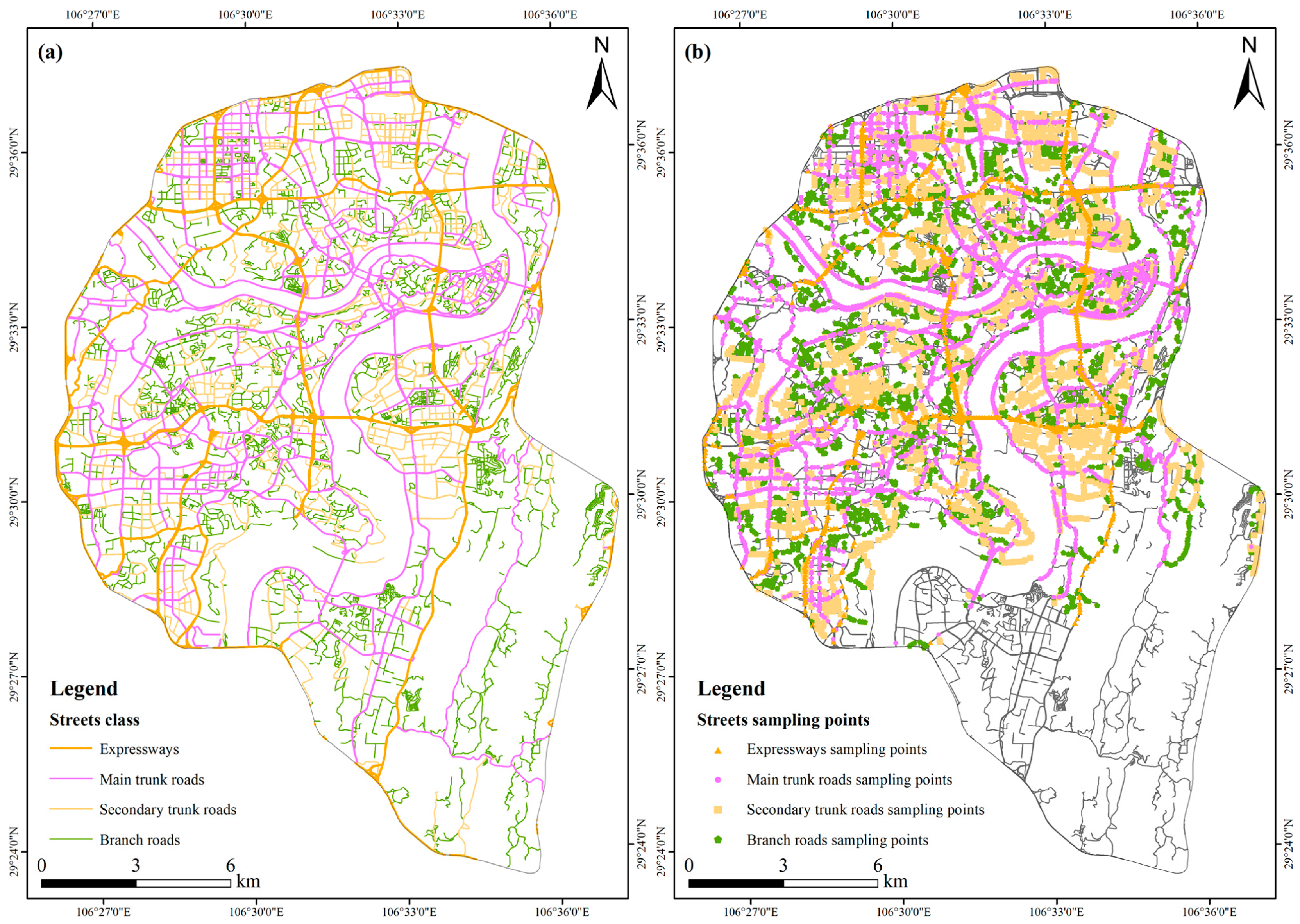
To get consistent locations of these datasets, firstly, locations of different street types were calibrated based on images from Google Earth images in 2019, and the software was downloaded from the 91weitu website (https://www.91wemap.com/) (accessed on 18 May 2021). The Google Earth images had a standard projection system with WGS_1984; however, the coordinates of the Baidu map had a slight deviation. Hence, Google Earth was set as a reference map to calibrate other datasets acquired from the Baidu map. Then, based on spatial analysis tools in ArcGIS 10.8 software, sampling points (a total of 15,862) of streetscape images every 100 m along the street line were generated, and the longitude and latitude coordinates of each sampling point were calculated; finally, Python was used to download Baidu Street View pictures from four directions of each sampling point (Figure 2). Except for the area not covered by Baidu Street View, a total of 60,586 Baidu Street View pictures were obtained. In this study, these extracted Baidu Street View pictures were acquired from June to August of 2019, which means that we could ignore the impact of the seasonal changes of plants on SGR.

2.3. Methods

The research methodology of this paper consisted of four main parts, which included the following: (1) the retrieval of LST; (2) the calculation of SGR; (3) the classification of street types; and (4) a correlation analysis. Section 2.3.1, Section 2.3.2, Section 2.3.3 and Section 2.3.4 present the calculation formula in detail.

2.3.1. Retrieval of LST

In the study of the urban heat islands effect, the monitoring of LST is one of the main methods to understand the spatial and temporal distribution characteristics of a heat island, and the LST retrieval based on satellite remote sensing images is the primary method. In recent years, satellite remote sensing images, including Landsat series, ASTER, MODIS, and other products, were used to retrieve LST [30]. Among them, Landsat 8 images launched in 2013 have the advantages of high spatial resolution, rich spectral information, and long-term monitoring. Hence, Landsat 8 images have been widely used [31,32]. To date, the single band algorithm and window splitting algorithm were the two main types in retrieving LST [33,34]. Specifically, the single band algorithm included the atmospheric correction method, single channel algorithm, image-based algorithm, and single window algorithm [35,36,37,38]. Among them, the atmospheric correction method, also named the radiative transfer equation method, is a traditional algorithm based on the atmospheric radiative transfer model. Its advantage lies in that it could be applied to any thermal infrared remote sensing band [39]. Equations (1)–(8) are calculation formulas.
L λ = [ ε B ( T s ) + ( 1 ε ) L d o w n ] τ + L u p
B ( T s ) = L λ L u p τ ( 1 ε ) L d o w n τ ε
T s = K 2 ln ( K 1 B ( T s ) + 1 )
ε = 0.004 P v + 0.986
P v = [ ( N D V I N D V I s o i l ) ( N D V I v e g N D V I s o i l ) ]
ε w a t e r = 0.995
ε s u r f a c e = 0.9625 + 0.0614 × P v 0.0461 × P v 2
ε b u i l d i n g = 0.9589 + 0.086 × P v 0.0671 × P v 2
where L λ denotes the thermal infrared radiation brightness value received by satellite sensor; L u p indicates the upwelling radiance of atmosphere; L d o w n represents the downwelling radiance of atmosphere; ε is the surface emissivity; τ is the atmospheric transmission at thermal infrared band; L u p , L d o w n and τ are acquired from NASA website (http://atmcorr.gsfc.nasa.gov/) (accessed on 23 August 2021) after inputting the time, latitude and longitude. In this study, their values equal 4.77 W / ( m 2 × μ m × sr ) , 7.06 W / ( m 2 × μ m × sr ) , and 0.44, respectively. T s is the actual surface temperature; B ( T s ) is the radiance brightness of the black body at temperature T s ; K1 and K2 are constant values with the value of 774.89 W / ( m 2 × μ m × sr ) and 1321.08 K, which are provided by the metadata file of the Landsat 8 image; P v represents the vegetation coverage, which is calculated based on N D V I index; N D V I v e g and N D V I s o i l represent the N D V I value of pure vegetation pixels and bare soil or no vegetation coverage pixels. In this study, the N D V I v e g and N D V I s o i l values are 0.70 and 0.05, respectively [40,41]; When the N D V I value at certain pixel is greater than 0.70, the value of P v equals 1.00, while the N D V I value at a certain pixel is less than 0.05, the value of P v equals 0.00. ε w a t e r , ε s u r f a c e and ε b u i l d i n g represent the surface emissivity of the water pixel, natural surface pixel, and urban area pixel, respectively.

2.3.2. Calculation of SGR

Based on Baidu Street View pictures, this study used the image semantic segmentation method to calculate each street’s SGR from four directions [42,43,44]. It included six steps, which were (1) the acquisition of the city street network; (2) the sampling points’ generation of street scene images per 100 m in street network; (3) the acquisition of Baidu Street View pictures of sampling points from four directions; (4) the semantic segmentation of Baidu Street View pictures based on a full convolution network; (5) the percentage calculation of vegetation pixels in each picture; and (6) the average value of the street-greenery rate from four directions. Figure 3 displays the calculation method of the SGR of the sampling point.

2.3.3. Classification of Street Types

A street’s thermal environment is affected by the climate environment of the surrounding areas. First, there is a significant correlation between the surface temperature and the density of urban impervious and underlying surfaces [45,46]; secondly, the spatial distribution of buildings in horizontal and vertical directions is extremely uneven. The buildings and narrow streets formed by the buildings will weaken the effect of heat diffusion, thus affecting the surface temperature [47]; thirdly, factors including the height-width ratio of a street, sky visibility, and building density are often used as the basis for the division of a local climate zone.
Hence, in this study, in the division of different street types, the concept of LCZ was introduced first, and the urban areas where the street was located were preliminarily divided by referring to the LCZ division method. The street types were then further distinguished according to the direction and street width. Specifically, LCZ was promoted by Stewart and Oke in 2012, and it referred to the area with the same surface coverage, similar spatial form, building materials, and similar human activities within the range of several hundred meters to several kilometers in one city [48,49]. Based on the concept of LCZ, it could be divided into 17 types [48]. Combined with the actual situation of the study area, the LCZ could be divided into ten types (Table 1).
Combined with the specific range of impervious surface fraction and pervious surface fraction proposed by Mills [49], the parameter range of block division is shown in Table 2.

2.3.4. Correlation Analysis

A correlation analysis is a statistical analysis method that is used to study the correlation between two or more random variables in the same position [50,51]. Equation (9) is the calculation formula.
R x y = i = 1 n i = 1 n ( x i x ¯ ) ( y i y ¯ ) i = 1 n i = 1 n ( x i x ¯ ) 2 i = 1 n i = 1 n ( y i y ¯ ) 2
where R x y denotes the correlation coefficient between x and y ; x i and y i are the LST and SGR at ith point; and x ¯ and y ¯ are the average value of LST and SGR.

3. Results

3.1. Spatial Characteristic of LST Result

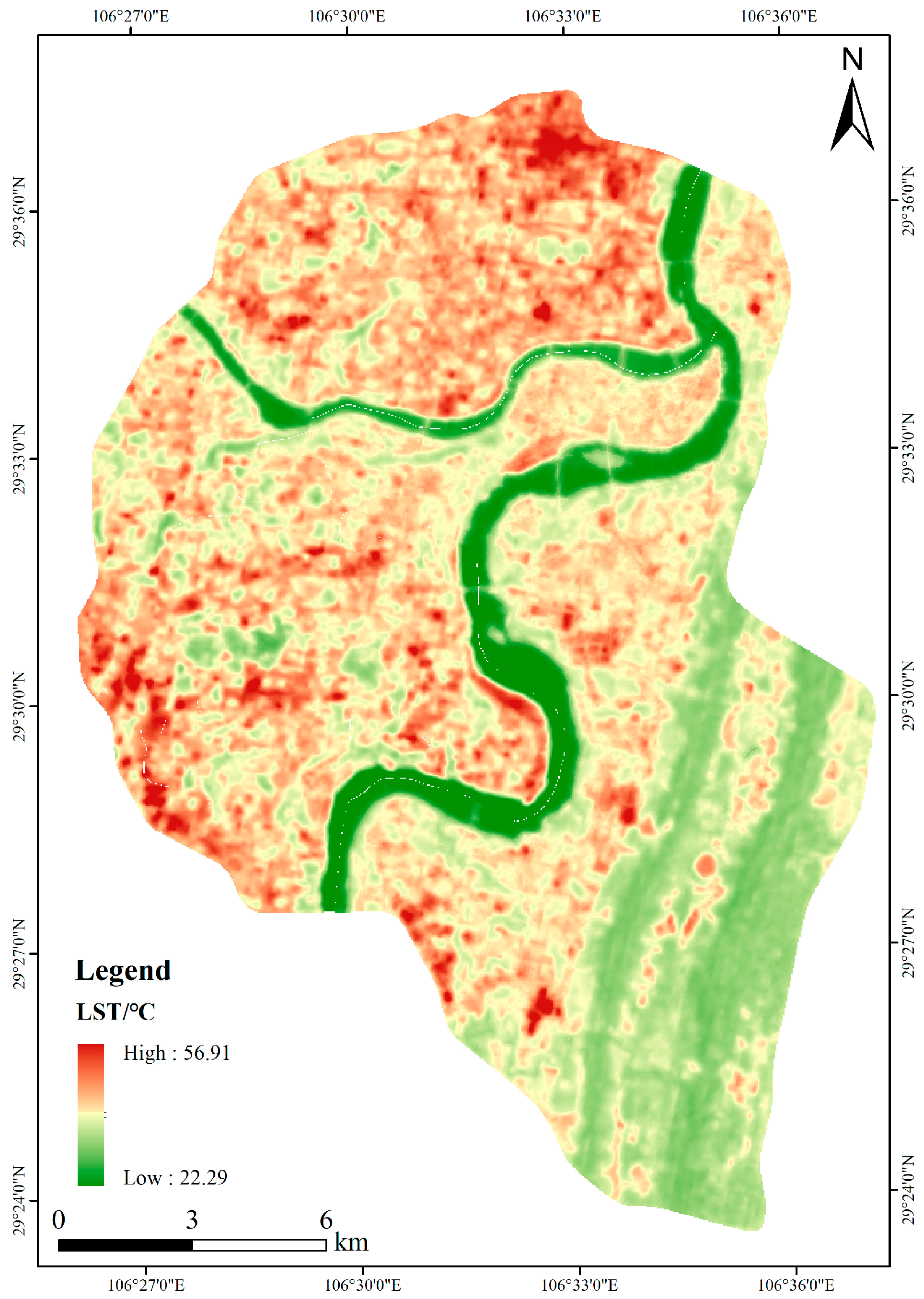
Based on the atmospheric correction method, the LST spatial distribution map was acquired on 20 August 2019 (Figure 4). In addition, combined with the application of the mean standard deviation division method in the previous study [42,52], this study used this method to divide the LST of the study area into five grades, which were high-temperature zone, sub-high temperature zone, middle-temperature zone, sub-middle temperature zone, and low-temperature zone (Figure 5).
According to Figure 4 and Figure 5, the high-temperature zones were mainly concentrated in the core commercial areas, dense residential areas, and industrial cluster areas. The LST spatial distribution patterns were closely related to human activities. Factors such as building height and surface materials would also affect the LST spatial distribution patterns. Reasonable urban planning, green space construction and other methods could effectively mitigate the heat island effect. However, for these built-up areas in the urban center, it was challenging to reserve large land areas for green space construction.

3.2. Spatial Distribution Map of Streets LST

Based on the calibrated street network data, the streets’ LST were extracted (Figure 6).
According to Figure 6, the streets with a high LST were mainly concentrated in the northern and western regions. The most severe regions with high temperatures were mostly around Chongqing North Railway Station. Based on satellite images, buildings in these regions were distributed densely, with many commercial and residential buildings. Streets with high LST in western regions were mainly located in Mawangchang and Hualong in the Jiulongpo District. Except for many residential buildings in these regions, there also existed many building material markets. The buildings in these markets mainly belonged to low-rise and large-area buildings, accompanied by a large area of hard paved ground. Streets with mid-level temperatures were primarily distributed in the Yuzhong Peninsula, the Nanping Business District, and the Shapingba Business District. These regions had dense buildings on both sides of the streets. Streets in these regions mainly belonged to the urban secondary trunk roads and branch roads. The shading effect of buildings on these streets was more evident than that of streets in high LST. Streets with low-temperature surfaces were mainly distributed on both sides of the river and in the eastern and southern regions. By comparing these streets’ LST on both sides of the river, it could be seen that these streets’ LST on the south bank of the river were significantly lower than those on the north bank of the river. This is because the rivers flowing through the city would reduce the air temperature of the surrounding environment, thus increasing the heat exchange between the surface and the air of the streets along the river and reducing street surface temperature. On the other hand, these north bank riverside streets absorbed a significant amount of solar radiation, causing their LSTs to be higher than those of the south bank riverside streets. The eastern and southern Chongqing belonged to mountainous areas (Nanshan), with high green coverage and low building density. Plant shading and transpiration affected the total amount of solar radiation entering these streets; hence, the air temperature on these streets was lower. Therefore, these streets’ LST were significantly lower than in other areas.
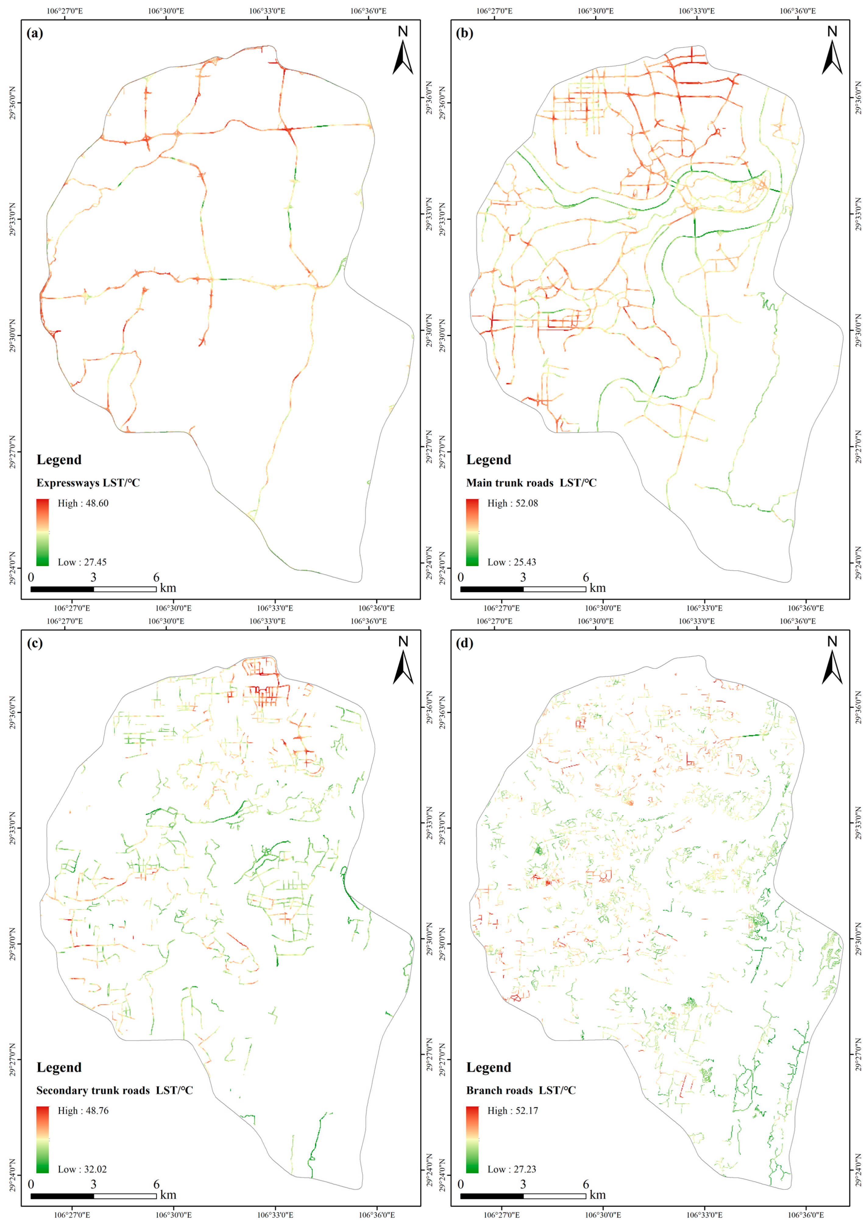
To further understand these streets’ LSTs of different types, the streets in the study area were divided into expressways, main trunk roads, secondary trunk roads, and branch roads (Figure 7).
According to Figure 7, the streets’ LST of expressways and main trunk roads were higher than the secondary trunk roads and branch roads. In addition, these streets’ width also exerted a specific influence on LST. Furthermore, the expressways and main trunk roads with high LST were mainly distributed in those streets with an east-west orientation, indicating that street orientation will affect the street LST.

3.3. Spatial Distribution of SGR

Figure 8 shows the spatial distribution of SGR in the study area.
According to Figure 8, the average value of the expressways’ SGR was 21.70%, and the average value of the main trunk roads’ SGR was 22.40%. As for the secondary trunk roads and branch roads, their average SGR values were 24.60% and 26.70%, respectively. Generally, the streets’ width will decrease the level of SGR. This is because the increase in a street’s width will lead to a more significant coverage of the field of view, and the proportion of plants in the field of view will decrease.

3.4. Spatial Distribution of Different Street Types

Figure 9 shows the spatial distribution of varying street types in the study area.
According to Figure 9, forest areas were mainly distributed in the southeastern regions. Waterbody areas were primarily located in the central regions. High-rise and low-density built-up areas, and high-rise and high-density built-up areas were dominant regions. Among them, high-rise and high-density built-up areas were mainly found along the waterbody areas. For sand grassland and bare areas, they were sporadically distributed in the southeastern regions. Generally, in the entire study area, high-rise built-up areas accounted for the highest percentage of all built-up types, followed by multi-rise areas. However, low-rise built-up areas accounted for the low rate.

4. Discussion

4.1. Validation of SGR Calculation Results

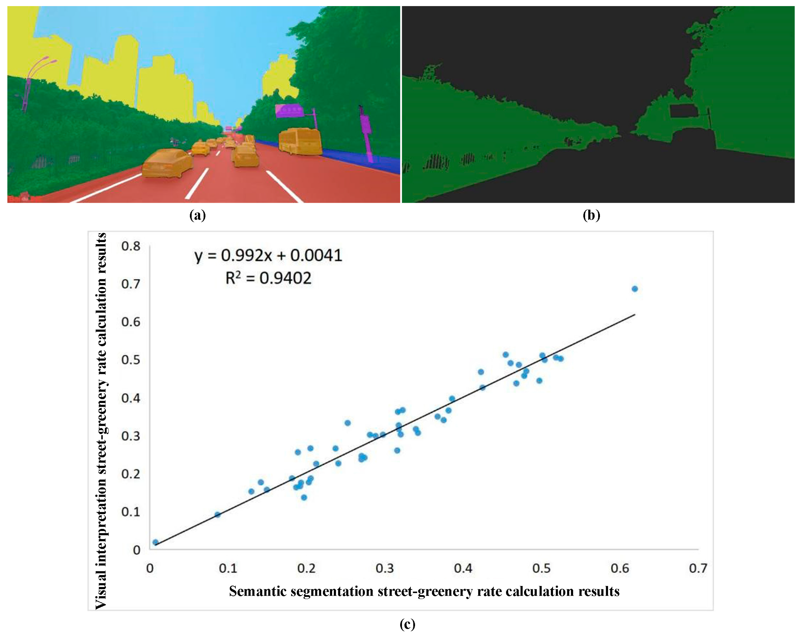
To validate the effectiveness of SGR calculation results, fifty Baidu Street View pictures were randomly selected to compare their SGR based on semantic segmentation and visual interpretation methods. Specifically, semantic segmentation methods based on the full convolution network were applied to all Baidu Street View pictures automatically, and the street-greenery rate of each picture was then calculated. For visual interpretation methods, these fifty selected pictures were digitalized, their SGR was calculated. Finally, a scatter plot was drawn between both methods (Figure 10).
The key in calculating SGR was the accurate detection of plants. According to Figure 10, both methods showed relatively good detection results, indicating that both methods displayed good consistency. However, there existed slight differences between the two methods. The shadow of plants may be recognized as other types based on the semantic segmentation method. However, objects in shadow areas could be accurately detected based on a visual interpretation. Generally, the SGR calculation result when the semantic segmentation method was used was accurate, with an R2 of 0.94.
To further validate the SGR results, the statistical results of SGR were calculated (Figure 11). The average SGR of the study area was 24.30%, which was higher than the global average value (19.03%) [53]. Based on the grading standard [28], this study divided the SGR into five grades, which were poor (0.0–5.0%), fair (5.0–15.0%), moderate (15.0–25.0%), good (25.0–35.0%), and excellent (≥35.0%). Combined with grading results, the proportion of streets with poor greening levels in the study area was 8.85%, the proportion of streets with fair greening levels was 16.97%, the proportion of streets with a moderate greening level was 23.53%, the proportion of streets with a good greening level was 24.21%, and the proportion of streets with an excellent greening level was 26.43%. The reasons for these streets having poor greening levels were because of the particular terrain. Chongqing is a mountainous city. The height difference in urban built-up regions varies greatly, which led to a higher proportion of tunnels and viaducts in the urban traffic system compared with more normal cities. In addition, the available space on both sides was less, which did not meet the requirements for street greening construction, thus leading to an increase in the proportion of low-green visibility streets within the study area.

4.2. Relationship Exploration between Streets’ SGR and LST

Based on the block division rule, the streets in different blocks were further divided according to street orientation and width. The streets could be divided into four types based on their width, which were expressways, main trunk roads, secondary trunk roads, and branch roads. In different block types, street orientation and street class were also taken into consideration. Finally, seventy-two street types were acquired. Table 3 displays the correlation coefficient between the streets’ SGR and LST at different types.
Given the influence sampling points, the correlation of these street types was not calculated with sampling points less than 50. Based on Table 3, there was a negative correlation between the SGR and the LST in most streets, but the correlation results in different regions were not the same. On the other hand, these street types with high correlation were the south-north expressways, main trunk roads, secondary trunk roads, and branch roads in multi-rise and low-density built-up areas. Among these four types of streets, street greening had the best cooling effect on their surface temperature.
Due to insufficient sampling points of low-rise built-up buildings in the study area, the correlation between streets’ SGR and LST was not calculated. Therefore, the comparative analysis was mainly conducted between multi-rise and high-rise built-up areas. Generally, whether the street orientation was south-north or east-west, the correlation coefficient in low-rise built-up areas was higher than in high-rise built-up areas. The buildings in low-density built-up areas provided less shading area for street space, and the blocking of solar radiation depended more on the shading effect of greening. Hence, the correlation between SGR and LST in multi-rise and low-density built-up areas was higher. Comparing streets with different street orientations in multi-rise and low-density built-up areas, the correlation between the streets’ SGR and LST in the south-north orientation was higher than in the east-west orientation. This was mainly because the shading area buildings of these streets with an east-west orientation could provide more shade. In addition, influenced by the prevailing southeast wind in summer, streets with a south-north orientation were more conducive to airflow. To these streets with a south-north orientation, the correlation between the streets’ SGR and LST in multi-rise and low-density built-up areas was higher than in high-rise and low-density built-up areas. This was mainly because the high-rise buildings could block more solar radiation compared with multi-rise buildings. Generally, the lower the height and density of buildings, the better the cooling effect of street greening. At the same time, the cooling effect of these streets with a south-north orientation was better than those with an east-west orientation. Therefore, in these streets, the LST could be reduced by increasing the SGR.
For these streets in low-rise and low-density built-up areas with a south-north orientation, fitting formulas of different road types were drawn (Figure 12).
Based on Figure 12, the fitting formula of expressways was y = −0.0426x + 1.9768, and R2 equaled 0.5445. According to this linear modeling result, the LST of this street type may be decreased by 1 °C when the SGR increased by 4.26%. The fitting formula of the main trunk road was y = −0.0345x + 1.6206, and R2 equaled 0.4969. According to this linear modeling result, the LST of this street type may be decreased by 1 °C when the SGR increased by 3.45%; The fitting formula of the secondary trunk roads was y = −0.0353x + 1.7024, R2 equaled 0.5027. According to this linear modeling result, the LST of this street type decreased by 1 °C when the SGR increased by 3.53%. The fitting formula of a branch road was y = −0.0303x + 1.5020, and R2 equaled 0.5282. According to this linear modeling result, the LST of this street type decreased by 1 °C when the SGR increased by 3.03%. Generally, with the increase of street SGR, the decrease in LST of the expressways was the largest, while that of branch roads was the smallest. However, the most significant difference between these four street types was the width. Therefore, the wider the street, the higher the cooling efficiency of plants. In addition, the average R2 of four different street types was 0.5181, and the streets’ LST in low-rise and low-density built-up areas with a south-north orientation decreased by 1°C when the SGR increased by 3.57%.

4.3. Policy Implications and Limitations

This study used multi-source datasets to explore the relationship between SGR and LST in different street types. Moreover, the street orientation and LCZ concept were also taken into consideration. Based on our results, streets with a south-north orientation, the height of buildings, and the width of a street exert an influence on the street greening effect. Based on the aforementioned results, for the streets in the multi-rise and low-density built-up areas with a south-north orientation, some suggestions were given: (1) Increase the continuity of greening; For these streets with uneven green distribution in the built-up area, new trees can be planted appropriately to build a complete “green corridor”; (2) Enrich the street greening configuration. The suitable combination of arbor, shrubs, and grass can enrich the spatial level of a street’s green belt. The upper layer of the multi-layer structure should be dominated by local tall trees, and the middle and lower layers should be dominated by shrubs and herbs with strong shade resistance. (3) Increase the vertical greening of streets. Vertical greening is also known as three-dimensional greening. Its advantage is that it uses less ground space to obtain more green viewing area, which can improve the environment more. Common vertical greening forms include wall greening, colonnade greening, etc. For the walls of buildings on both sides of the street, the characteristics of climbing plants can be used to achieve green coverage of the building surface during their growth. In addition, planting containers can be installed on the wall surface to achieve green coverage of the wall. (4) The appropriate tree species need to be selected. From the analysis results of the street green sight rate, it can be concluded that the crown width of trees has an essential impact on the street green sight rate. Therefore, within the allowable range of street widths, the green sight rate can be improved by planting trees with a larger crown width and higher leaf density. In tree species selection, local trees with better adaptability to the environment should be the main species, and the proportion of evergreen and deciduous trees should be reasonably allocated.
This study investigated the relationship between streets’ SGR and LST by introducing LCZ. However, there are still some limitations to this study. Firstly, the daytime LST data was acquired to explore its relationship with SGR. However, to further investigate the relationship between streets’ LST and SGR, LST at nighttime should also be used in the consideration of their relationship. Secondly, building data was obtained from Baidu Maps; however, there were differences between the obtained building data and the actual situation. Although building data were calibrated based on Google Earth images, it is difficult to acquire building data with high precision. Finally, the heat produced by human activity in these streets was not taken into consideration, as it was difficult to quantify.

5. Conclusions

Relationship exploration between streets’ SGR and LST of different types is of great significance for realizing regional sustainable development goals. Given the lack of consideration of the LCZ concept, Chongqing’s Inner Ring region was used to assess the relationship between the streets’ SGR and LST. First, the LST was retrieved from Landsat 8 imagery after atmospheric correction; next, the SGR of different streets was calculated based on the semantic segmentation method; finally, street types were classified in detail by introducing LCZ, and the relationship between SGR and LST was explored. The results showed that: (1) The LST spatial distribution pattern was closely related to human activity, with the high-temperature zones mainly concentrated in the core commercial areas, dense residential areas, and industrial cluster areas; (2) The average SGR values of expressways, main trunk roads, secondary trunk roads, and branch roads were 21.70%, 22.40%, 24.60%, and 26.70%, respectively. The level of SGR will decrease when the street width increases; (3) There is a negative correlation between the SGR and the LST in most streets. Among them, the LST of secondary trunk roads in low-rise and low-density built-up areas with a south-north orientation had a strong negative correlation with the SGR. Moreover, the wider the street, the higher the cooling efficiency of plants. Specifically, the LST of streets in low-rise and low-density built-up areas with a south-north orientation decreased by 1 °C when the street-greenery rate increased by 3.57%.

Author Contributions

Conceptualization, X.W. and H.Q.; methodology, S.D.; software, S.D. and Z.L.; validation, X.S. and H.Q.; formal analysis, X.W.; investigation, R.Z.; resources, S.D. and H.Q.; data curation, X.W. and Z.L.; writing—original draft preparation, X.W.; writing—review and editing, J.J.; visualization, X.W. and S.D.; supervision, H.Q.; project administration, H.Q. and X.S.; funding acquisition, H.Q. and X.S. All authors have read and agreed to the published version of the manuscript.

Funding

This research was funded by the Chongqing City Administration Bureau (Name: Study on Landscape Evaluation and Quality Improvement of Street Trees in Chongqing, No. CGK2019024).

Institutional Review Board Statement

Not applicable.

Informed Consent Statement

Not applicable.

Data Availability Statement

The data presented in this study are available on request from the corresponding author.

Acknowledgments

We thank the National Geomatics Center of China, Baidu Maps, the Geospatial Data Cloud, and the Chongqing Meteorological Service for supplying the administrative division data, remote sensing dataset, meteorological data, road network data, and Baidu Street View pictures.

Conflicts of Interest

The authors declare that they have no conflicts of interest.

Abbreviations

LCZLocal climate zoneA term for describing regional local climate
LSTLand surface temperatureAn index for describing regional surface temperature
SGRStreet-greenery rateAn index for describing the street greenery rate

References

  1. Wen, Q.; Zhang, Z.; Shi, L.; Zhao, X.; Liu, F.; Xu, J.; Yi, L.; Liu, B.; Wang, X.; Zuo, L.; et al. Extraction of basic trends of urban expansion in China over past 40 years from satellite images. Chin. Geogr. Sci. 2016, 26, 129–142. [Google Scholar] [CrossRef]
  2. National Bureau of Statistics of the People’s Republic of China. China Statistical Yearbook; China Statistics Press: Beijing, China, 2022. [Google Scholar]
  3. United Nations, Department of Economic and Social Affairs, Population Division. World Urbanization Prospects: The 2018 Revision; United Nations, Department of Economic and Social Affairs, Population Division: New York City, NY, USA, 2018. [Google Scholar]
  4. Ahmed, G.; Zan, M.; Kasimu, A. Spatio-Temporal Changes and Influencing Factors of Surface Temperature in Urumqi City Based on Multi-Source Data. Environ. Eng. Sci. 2022, 39, 928–939. [Google Scholar] [CrossRef]
  5. Morshed, M.; Chakraborty, T.; Mazumder, T. Measuring Dhaka’s urban transformation using nighttime light data. J. Geovis. Spat. Anal. 2022, 6, 25. [Google Scholar] [CrossRef]
  6. Zhang, W.; Li, Y.; Zheng, C.; Zhu, Y. Surface urban heat island effect and its driving factors for all the cities in China: Based on a new batch processing method. Ecol. Indic. 2023, 146, 109818. [Google Scholar] [CrossRef]
  7. Badugu, A.; Arunab, K.S.; Mathew, A.; Sarwesh, P. Spatial and temporal analysis of urban heat island effect over Tiruchirappalli city using geospatial technuques. Geod. Geodyn. 2022, in press. [CrossRef]
  8. Feng, R.; Wang, F.; Liu, S.; Qi, W.; Zhao, Y.; Wang, Y. How urban ecological land affects resident heat exposure: Evidence from the mega-urban agglomeration in China. Landsc. Urban Plan. 2023, 231, 104643. [Google Scholar] [CrossRef]
  9. Li, H.; Zhou, W.; Wang, W.; Zheng, Z. Imbalanced supply and demand of temperature regulation service provided by urban forests: A case study in Shenzhen, China. Ecol. Indic. 2022, 145, 109666. [Google Scholar] [CrossRef]
  10. Li, X.; Zhang, C.; Li, W.; Ricard, R.; Meng, Q.; Zhang, W. Assessing street-level urban greenery using Google Street View and a modified green view index. Urban For. Urban Green. 2015, 14, 675–685. [Google Scholar] [CrossRef]
  11. Xiao, L.; Wang, W.; Ren, Z.; Fu, Y.; Lv, H.; He, X. Two-city street-view greenery variations and association with forest attributes and landscape metrics in NE China. Landsc. Ecol. 2021, 36, 1261–1280. [Google Scholar] [CrossRef]
  12. Souverijns, N.; Ridder, K.; Veldeman, N.; Lefebre, F.; Kusambiza-Kiingi, F.; Memela, W.; Jones, N. Urban heat in Johannesbrug and Ekurhuleni, South Africa: A meter-scale assessment and vulnerability analysis. Urban Clim. 2022, 46, 101331. [Google Scholar] [CrossRef]
  13. Xu, X.; Pei, H.; Wang, C.; Xu, Q.; Xie, H.; Jin, Y.; Feng, Y.; Tong, X.; Xiao, C. Long-term analysis of the urban heat island effect using multisource Landsat images considering inter-class differences in land surface temperature products. Sci. Total Environ. 2023, 858, 159777. [Google Scholar] [CrossRef]
  14. Wang, Z.; Zhang, A.; Liu, M. Daily Spatial Distribution of Apparent Temperature Comfort Zone in China Based on Heat Index. Remote Sens. 2022, 14, 4999. [Google Scholar] [CrossRef]
  15. Huang, Y.; Sun, Y. Judgement Characteristics and Quantitative Index of Suitable Block Scale. J. South China Uni. Technol. 2012, 40, 131–138. [Google Scholar]
  16. Jin, J. Research of Three-Dimensional Numerical Simulation of Outdoor Thermal Environment on Block-Scale. Zhejiang University. 2010. Available online: https://kns.cnki.net/KCMS/detail/detail.aspx?dbname=CMFD2010&filename=2010125235.nh (accessed on 1 March 2020).
  17. Du, X. Study on Design Strategy for Thermal Environments of Living Street Canyons in Guangzhou. South China University of Technology. 2014. Available online: https://kns.cnki.net/KCMS/detail/detail.aspx?dbname=CMFD201501&filename=1014063622.nh (accessed on 1 March 2020).
  18. Zhou, W.; Tian, Y. Effects of urban three-dimensional morphology on thermal environment: A review. Acta Ecol. Sin. 2020, 40, 416–427. [Google Scholar]
  19. Ding, W.; Hu, Y.; Dou, P. Study on Interrelationship between Urban Pattern and Urban Microclimate. Agchit. J. 2012, 7, 16–21. [Google Scholar]
  20. Steemers, K. Energy and the city: Density, buildings and transport. Energy Build. 2003, 35, 3–14. [Google Scholar] [CrossRef]
  21. Cao, A. Road Type of Remote Sensing and the Simulation Analysis of the Impact of Urban Thermal Environment. South China University of Technology. 2016. Available online: https://kns.cnki.net/KCMS/detail/detail.aspx?dbname=CMFD201701&filename=1016771415.nh (accessed on 1 March 2020).
  22. Ali-Toudert, F.; Mayer, H. Effects of asymmetry, galleries, overhanging facades and vegetation on thermal comfort in urban street canyons. Sol. Energy 2006, 81, 742–754. [Google Scholar] [CrossRef]
  23. Bourbia, F.; Awbi, H.B. Building cluster and shading in urban canyon for hot dry climate. Renew. Energy 2004, 29, 291–301. [Google Scholar] [CrossRef]
  24. Daniel, C.; Mathew, S.; Subbarayan, S. GIS-based study on the association between road centrality and socio-demographic parameters: A case study. J. Geovis. Spat. Anal. 2022, 6, 1–12. [Google Scholar] [CrossRef]
  25. Wu, L. Research on Urban Road Green Space Design Based on the Green Looking Ratio. Shanghai Jiaotong University. 2008. Available online: https://kns.cnki.net/KCMS/detail/detail.aspx?dbname=CMFD2008&filename=2008054618.nh (accessed on 1 March 2020).
  26. Zhao, S.; Liang, Q.; Zhou, X.; Su, B. Application of Green Looking Ratio in Urban Road Greenland Design. Chin. Hortic. Abstr. 2010, 7, 97–99. [Google Scholar]
  27. Feng, S.; Wei, Y.; Wang, Z.; Yu, X. Pedestrian-view urban street vegetation monitoring using Baidu Street View images. Chin. J. Plant Ecol. 2020, 44, 205–213. [Google Scholar] [CrossRef]
  28. Xu, B.; Yang, F.; Li, L. On Green Vision Rate of Road in Old Town of Zhengzhou City Based on Image Recognition. J. Southwest China N. Univ. 2020, 45, 113–119. [Google Scholar]
  29. Hu, P. Study on Urban Heat Island in the Central City of Chengdu Based on Landsat 8. Chengdu University of Technology. 2015. Available online: https://kns.cnki.net/KCMS/detail/detail.aspx?dbname=CMFD201601&filename=1015312188.nh (accessed on 1 March 2020).
  30. Li, F.; Ma, A.; Ding, Y.; Yang, J.; Jiao, J.; Liu, L. Research on Urban Heat Island Effect Based on Landsat Data. Remote Sens. Technol. Appl. 2009, 24, 553–558. [Google Scholar]
  31. Zhang, Z.; He, G.; Wang, M.; Long, T.; Wang, G.; Zhang, X.; Jiao, W. Towards an operational method for land surface temperature retrieval from Landsat 8 data. Remote Sens. Lett. 2016, 7, 279–288. [Google Scholar] [CrossRef]
  32. Li, S.; Wang, J.; Li, D.; Ran, Z.; Yang, B. Evaluation of Landsat 8-like Land Surface Temperature by Fusing Landsat 8 and MODIS Land Surface Temperature Product. Processes 2021, 9, 2262. [Google Scholar] [CrossRef]
  33. Zhu, X.; Duan, S.; Li, Z.; Wu, P.; Wu, H.; Zhao, W.; Qian, Y. Reconstruction of land surface temperature under cloudy conditions from Landsat 8 data using annual temperature cycle model. Remote Sens. Environ. 2022, 281, 113261. [Google Scholar] [CrossRef]
  34. Fu, Y.; Guo, Q.; Wu, X.; He, C.; Sang, X.; Xie, T. A modified model of surface temperature inversion based on Landsat 8 remote-sensing data and measured data. Int. J. Remote Sens. 2018, 39, 6170–6181. [Google Scholar] [CrossRef]
  35. Onačillová, K.; Gallay, M.; Paluba, D.; Péliová, A.; Tokarčík, O.; Laubertová, D. Combining Landsat 8 and Sentinel-2 Data in Google Earth Engine to Derive Higher Resolution Land Surface Temperature Maps in Urban Environment. Remote Sens. 2022, 14, 4076. [Google Scholar] [CrossRef]
  36. Meng, X.; Cheng, J. Evaluating Eight Global Reanalysis Products for Atmospheric Correction of Thermal Infrared Sensor—Application to Landsat 8 TIRS10 Data. Remote Sens. 2018, 10, 474. [Google Scholar] [CrossRef]
  37. Guo, Y.; Zhang, C. Analysis of Driving Force and Driving Mechanism of the Spatial Change of LST Based on Landsat 8. J. Indian Soc. Remote 2022, 50, 1787–1801. [Google Scholar] [CrossRef]
  38. Sekertekin, A.; Bonafoni, S. Sensitivity Analysis and Validation of Daytime and Nighttime Land Surface Temperature Retrievals from Landsat 8 Using Different Algorithms and Emissivity Models. Remote Sens. 2020, 12, 2776. [Google Scholar] [CrossRef]
  39. García, D. Analysis and precision of the Terrestrial Surface Temperature using Landsat 8 and Sentinel 3 images: Study applied to the city of Granada (Spain). Sustain. Cities Soc. 2021, 71, 102980. [Google Scholar] [CrossRef]
  40. Digavinti, J.; Manikiam, B. Satellite monitoring of forest fire impact and regeneration using NDVI and LST. J. Appl. Remote Sens. 2021, 15, 042412. [Google Scholar] [CrossRef]
  41. Darge, Y.; Hailu, B.; Muluneh, A.; Kidane, T. Detection of geothermal anomalies using Landsat 8 TIRS data in Tulu Moye geothermal prospect, Main Ethiopian Rift. Int. J. Appl. Earth Obs. 2019, 74, 16–26. [Google Scholar] [CrossRef]
  42. Chen, S.; Wang, T. Comparison Analyses of Equal Interval Method and Mean-standard Deviation Method Used to Delimitate Urban Heat Island. J. Geo-Inf. Sci. 2009, 11, 145–150. [Google Scholar] [CrossRef]
  43. Hinton, G.; Salakhutdinov, R. Reducing the dimensionality of data with neural networks. Science 2006, 313, 504–507. [Google Scholar] [CrossRef] [Green Version]
  44. Tian, X.; Wang, L.; Ding, Q. Review of image semantic segmentation based on deep learning. J. Softw. 2019, 30, 440–468. [Google Scholar]
  45. Song, J.; Du, S.; Feng, X.; Guo, L. The relationships between landscape compositions and land surface temperature: Quantifying their resolution sensitivity with spatial regression models. Landsc. Urban Plan. 2014, 123, 145–157. [Google Scholar] [CrossRef]
  46. Zhou, W.; Wang, J.; Cadenasso, M. Effects of spatial configuration of trees on urban heat mitigation: A comparative study. Remote Sens. Environ. 2017, 195, 1–12. [Google Scholar] [CrossRef]
  47. Feng, Z.; Wang, S.; Jin, S.; Yang, J. Effects of urban morphology and wind conditions on land surface temperature in Changchun. Acta Geogr. Sin. 2019, 74, 902–911. [Google Scholar]
  48. Stewart, I.; Oke, T. Local climate zones for urban temperature studies. Bull. Am. Meteorol. Soc. 2012, 93, 1879–1900. [Google Scholar] [CrossRef]
  49. Zhou, Y. Study on the Construction of Urban Heat Island Maps of Shenzhen Based on Local Climate Zone. Harbin Institute of Technology. 2016. Available online: https://kns.cnki.net/KCMS/detail/detail.aspx?dbname=CMFD201801&filename=1017738684.nh (accessed on 1 March 2020).
  50. Kong, B.; Yu, H.; Du, R.; Wang, Q. Quantitative Estimation of Biomass of Alpine Grasslands Using Hyperspectral Remote Sensing. Rangeland Ecol. Manag. 2019, 27, 336–346. [Google Scholar] [CrossRef]
  51. Tang, F.; Xu, H. Impervious Surface Information Extraction Based on Hyperspectral Remote Sensing Imagery. Remote Sens. 2017, 9, 550. [Google Scholar] [CrossRef] [Green Version]
  52. Zhang, Z.; He, G.; Xiao, R.; Wang, W. A study of the urban heat island changes of Beijing city based on remote sensing. Remote Sens. Inform. 2005, 46–48. [Google Scholar]
  53. Cui, Z.; He, M.; Lu, M. An analysis of Green View Index in Cold Region City: A case study of Harbin. J. Chin. Urban Forest. 2018, 16, 34–38. [Google Scholar]
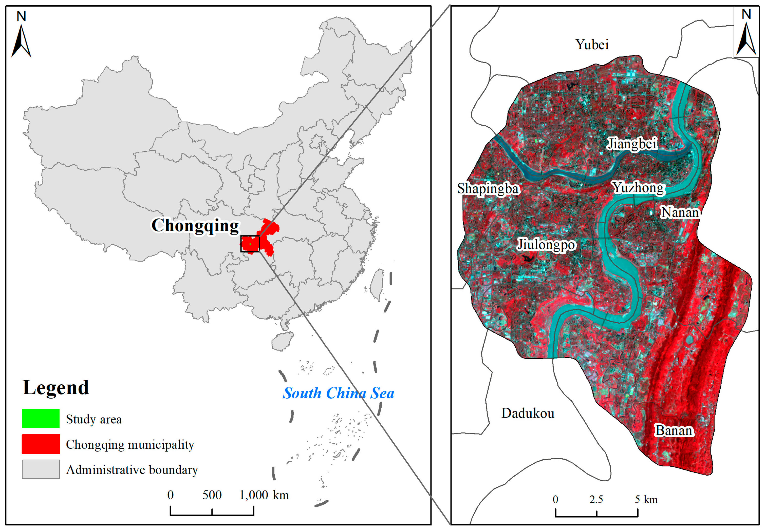
Figure 1. Location of the study area.
Ijerph 20 03294 g001
Figure 2. Spatial distribution map of streets in the study area (a), street sampling points in the study area (b).
Ijerph 20 03294 g002
Figure 3. SGR calculation steps of sampling points.
Ijerph 20 03294 g003
Figure 4. LST result based on the atmospheric correction method.
Ijerph 20 03294 g004
Figure 5. Different LST grades.
Ijerph 20 03294 g005
Figure 6. Spatial distribution map of streets LST.
Ijerph 20 03294 g006
Figure 7. Spatial distribution map of streets’ LST of different types: (a) Expressways; (b) Main trunk roads; (c) Secondary trunk roads; (d) Branch roads.
Ijerph 20 03294 g007
Figure 8. Spatial distribution map of SGR.
Ijerph 20 03294 g008
Figure 9. Spatial distribution of different street types.
Ijerph 20 03294 g009
Figure 10. Comparison of two SGR calculation methods: (a) Semantic segmentation result; (b) Visual interpretation result; (c) Scatter plot between two methods.
Ijerph 20 03294 g010
Figure 11. Statistical results of sampling points of the street-greenery rate.
Ijerph 20 03294 g011
Figure 12. Relationship between the streets SGR and LST of different types in multi-rise and low-density built-up areas, (a) Expressways; (b) Main trunk roads; (c) Secondary trunk roads; (d) Branch roads.
Ijerph 20 03294 g012
Table 1. LCZ types of the study area.
TypeSample
High-rise and high-density built-up areaIjerph 20 03294 i001
Multi-rise and high-density built-up areaIjerph 20 03294 i002
Low-rise and high-density built-up areaIjerph 20 03294 i003
High-rise and low-density built-up areaIjerph 20 03294 i004
Multi-rise and low-density built-up areaIjerph 20 03294 i005
Low-rise and low-density built-up areaIjerph 20 03294 i006
Forest areaIjerph 20 03294 i007
Sand grassland and bare areaIjerph 20 03294 i008
Hard ground areaIjerph 20 03294 i009
Waterbody areaIjerph 20 03294 i010
Table 2. Range of different block division parameters.
Block TypeAverage Building Height/mPervious Surface Fraction/%Building Density/%Impervious Surface Fraction/%
High-rise and high-density built-up area≥30<10≥2040–60
Multi-rise and high-density built-up area10–30<20≥2030–50
Low-rise and high-density built-up area<10<30≥2020–50
High-rise and low-density built-up area≥3030–405–2030–40
Multi-rise and low-density built-up area10–3020–405–2030–50
Low-rise and low-density built-up area<1030–605–2020–50
Forest area->90<5<10
Sand grassland and bare area->90<5<10
Hard ground area-<10<5>90
Waterbody area->90<5<10
Table 3. The correlation coefficient between the streets’ SGR and LST at different types.
Block TypeStreet TypeStreet OrientationPearson Correlation CoefficientSampling Points
High-rise and high-density built-up areaExpresswaySouth-north−0.20368
East-west−0.611 **100
Main trunk roadSouth-north0.003535
East-west−0.085 *531
Secondary trunk roadSouth-north−0.227 **489
East-west−0.136**463
Branch roadSouth-north−0.194 **653
East-west−0.060381
Multi-rise and high-density built-up areaExpresswaySouth-north−0.360 **59
East-west−0.06720
Main trunk roadSouth-north−0.224 **220
East-west0.007160
Secondary trunk roadSouth-north−0.264 **153
East-west0.022158
Branch roadSouth-north−0.228 **201
East-west−0.273 **112
Low-rise and high-density built-up areaExpresswaySouth-north/0
East-west/0
Main trunk roadSouth-north−0.916 **9
East-west/0
Secondary trunk roadSouth-north−0.8133
East-west/2
Branch roadSouth-north/1
East-west−0.9304
High-rise and low-density built-up areaExpresswaySouth-north−0.401 **294
East-west−0.17465
Main trunk roadSouth-north−0.253 **931
East-west−0.167 **792
Secondary trunk roadSouth-north−0.256 **578
East-west−0.246 **570
Branch roadSouth-north−0.335 **431
East-west−0.310 **268
Multi-rise and low-density built-up areaExpresswaySouth-north−0.738 **72
East-west−0.17465
Main trunk roadSouth-north−0.705 **412
East-west−0.092368
Secondary trunk roadSouth-north−0.709 **246
East-west−0.226 **207
Branch roadSouth-north−0.727 **167
East-west−0.335 **112
Low-rise and low-density built-up areaExpresswaySouth-north/0
East-west/0
Main trunk roadSouth-north−0.17156
East-west0.07323
Secondary trunk roadSouth-north−0.882 **16
East-west0.673 **14
Branch roadSouth-north−0.12918
East-west−0.664 **16
Forest areaExpresswaySouth-north−0.620 *16
East-west−0.476 *19
Main trunk roadSouth-north−0.165*151
East-west0.18664
Secondary trunk roadSouth-north−0.24562
East-west−0.356 **52
Branch roadSouth-north−0.10446
East-west−0.493 *22
Sand grassland and bare areaExpresswaySouth-north0.505 *16
East-west0.8403
Main trunk roadSouth-north0.023107
East-west−0.00869
Secondary trunk roadSouth-north0.04161
East-west−0.792 **25
Branch roadSouth-north0.01025
East-west−0.34916
Hard ground areaExpresswaySouth-north−0.326 **122
East-west−0.478 **104
Main trunk roadSouth-north−0.183 **315
East-west−0.054165
Secondary trunk roadSouth-north−0.484 **93
East-west−0.474 **94
Branch roadSouth-north−0.17377
East-west−0.32536
Note: * shows that the Pearson correlation coefficient of this type of street has passed the significance test of 95% confidence level; ** shows that the Pearson correlation coefficient of this type of street has passed the significance test of 99% confidence level.
Disclaimer/Publisher’s Note: The statements, opinions and data contained in all publications are solely those of the individual author(s) and contributor(s) and not of MDPI and/or the editor(s). MDPI and/or the editor(s) disclaim responsibility for any injury to people or property resulting from any ideas, methods, instructions or products referred to in the content.