Although the regulatory community focuses largely on MNs, an understanding of the reported environmental behavior of other suspended matter may lend insights into the likely environmental behavior of MNs. For example, estimated atmospheric residence times for reactive and unreactive gases range from 10⁷ years (e.g., He) to 10⁻² years (Rn, H₂O) [6]. In contrast:

These observations suggest that should a significant atmospheric MN emission occur, rapid aggregation may ensue and atmospheric residence times of 10 to 20 days may be typical. Particle deposition presumably occurs through both wet and dry deposition processes, although Lerman [11] indicates that dry deposition predominates in many cases. If one assumes an average near-surface atmospheric windspeed of 2.2 m/s [6], then those emissions entrained in an atmospheric air mass could travel up to ~1,900 km in 10 days.

Modeling the transport of colloidal material in aquatic systems may be more problematic. The literature suggests that colloids may be more mobile in ground waters at ionic strengths less than 0.001 M [12]. In addition, Degueldre et al. [13] published statistical relationships documenting that the stability of colloidal suspensions in natural waters is sensitive to the chemical composition of the water; in particular, they observe that maximum rates of particle aggregation occur at total dissolved salt contents equal to or greater than 0.01 molar (M) or at alkaline earth metal concentrations in excess of 0.0001 M. Assuming that these observations are applicable to environmental aqueous MN suspensions, aquatic MN transport in a stable colloidal suspension would most likely occur in rainwater and low ionic strength freshwaters [14,15].

Another issue is whether or not the environmental introduction of MNs may lead to the formation of stable aquatic colloidal suspensions. For example, Zhang et al. [16] found that SiO₂ was the only synthesized nanomaterial out of a collection of TiO₂, SiO₂, Fe₂O₃, ZnO, and NiO products that did not aggregate in pH 8.2 tap water at an ionic strength of less than 5×10⁻⁶ M. Thus, even upon their introduction into the environment, it is not clear that many of these products would necessarily experience aquatic transport as stable colloidal suspensions.

The transport of MNs associated with natural soils/sediments is a potentially significant environmental transport (and exposure) mechanism. However, as with our understanding of MN toxicological and environmental fate properties, developing procedures to understand those phenomena leading to MN solid/water partitioning is extremely challenging. For example, the filtration of water column samples may well composite suspended particulate matter that is not necessarily associated in the natural state. In addition, as will be demonstrated, MNs are likely to display relatively slow kinetics with respect to adsorption onto environmental solid phases (when compared to truly dissolved species); hence only systems of prolonged duration may begin to exhibit solid/water partitioning phenomena that are customarily attributed to thermodynamic equilibrium processes. Lastly, there are well recognized experimental difficulties associated with measuring those quantities of MNs associated with soils, sediments and sewage sludges and this represents yet another area of active research. Once reliable procedures become available for estimating MN solid/water partition coefficients, this potential exposure pathway is perhaps more amenable to simulation via a large variety of soil/sediment transport models that are and have been under development for many decades [17].

Models describing the intermedium transport behavior of contaminants with an acceptable degree of uncertainty are needed to assess the overall environmental fate and transport of potentially significant commercial products. In particular, it is necessary to adequately assess the air/water [18], air/solid [19], and solid/water [20] partitioning behavior of new products upon their introduction into environmental systems. Traditional approaches rely on air/solid partition coefficients (K_SAs), air/water (Henry’s Law) partition coefficients, and solid/water partition coefficients (K_ds). Theoretically these partition coefficients are based on an equilibrium partitioning concept. Specifically, given an appropriate equilibration period, the concentration ratio of a given material in any two phases in contact is presumed to approach a constant value. In systems where the assumption of equilibrium is not valid, one must resort to kinetic approaches for assessing intermedium transport. As an example, Jafvert and Kulkarni [21] measured the octanol/water partition coefficient (K_ow; where K_ow = C_octanol/C_water and the subscripted C’s designate concentrations in each phase) of nanoparticulate buckminsterfullerene (a spherical cage of sixty carbon atoms [C₆₀] that is approximately 1 nm in diameter). The authors employed a room temperature equilibration period of 4 to 13 days. A 4 to 13 day period to reach equilibration may be too long in some environmental transport scenarios. Moreover, as buckminsterfullerene particles may be among the smallest of MNs in commercial production, a 4 to 13 day equilibration period also may be too short to attain equilibrium with MNs possessing larger dimensions. In summary, kinetic models may be necessary for predicting MN fate, transport and exposures to the biosphere.

There are a number of examples of the significant influence that their high specific surface areas exert on MN properties. Nanoparticles possess a much larger fraction of constituents on the surface when compared to corresponding, consolidated larger-grain bulk material [22]. As surficial constituents have fewer bonds than do those in the bulk interior, they exist in higher-energy, less stable states. Because of this phenomenon, it was demonstrated, for example, that the melting point of cadmium sulfide (CdS) decreased from ~1200 °K to ~600 °K when CdS particle radii decreased from 3.5 nm to 1.5 nm [22].

In addition, the significance of interfacial tension and particle specific surface area/radius on the aqueous solubility of the material has been discussed by numerous authors. For example, Stumm and Morgan [23] published the following expression:

where log(K_{sp, SSA}) is the logarithm of the solubility product of a material with a specific surface area SSA, log(K_{sp, SSA=0}) is the logarithm of the solubility product of the bulk material, γ is the solid water interfacial tension, R is the ideal gas constant and T is the absolute temperature. The net effect is that depending on the interfacial tension, in many cases fine nanoparticles will be far more soluble than larger-sized particles of the same composition. Specifically, even if a potentially toxic bulk material is too insoluble to lead to dissolved concentrations of toxicological concern, the same cannot necessarily be said for the same material in the nanoparticulate state.

Another phenomenon associated with high specific surface areas (and very small radii) is that the pressure inside of small spherical bubbles is much higher than in the corresponding atmosphere [11,24]. Davies and Rideal [24] published the following expression for estimating the excess pressure, P_excess, inside of a bubble of radius r:

where γ represents the interfacial tension. This phenomenon is responsible for the common observation that surficial ocean waters are frequently supersaturated with respect to atmospheric gases (i.e., during wave activity very small bubbles are entrained in surface waters that acquire very high pressures and hence introduce dissolved gas concentrations much higher than would be expected from atmospheric equilibrium estimates). This phenomenon may be relevant to the environmental fate and persistence of nanometer sized atmospheric aerosols.

Lastly, the high specific surfaces areas associated with MNs will enhance any reactions dependent on the number of exposed sites. Concerns about dust explosions from finely ground coal, flour, sugar or other combustible products illustrate the significance of high specific surface areas associated with small particulate matter in commercial operations [25].

In quiescent fluid systems without turbulence, applications of Fick’s first law relate the one dimensional transport (flux) of a diffusing compound (F; in units of g/m²s) to an observed concentration gradient (dC/dz; in units of g/[cm³cm]) via a diffusivity coefficient D:

with this notation, Equation (3) can be rearranged to illustrate that the diffusivity coefficient D may be defined in units of cm²/s.

Equation (3) is applicable in quiescent, laminar, stagnant systems where turbulent transport of the suspending fluid is insignificant. In systems where rapid, turbulent flow exists, the consequent eddies and vortices also transport (and disperse) all dissolved and suspended materials that are contained within the fluid volume. As with atomic/molecular diffusion coefficients, the associated macroscopic coefficients that account for turbulent dispersion also may have units of cm²/s.

Table 1 compares literature-reported diffusivity values for atomic/molecular species in air and water with dispersivity coefficients in the same media. In addition, through application of the Stokes-Einstein equation, diffusivity estimates for MNs in water with radii of 0.5 nm to 50 nm are also presented. Lerman [11] suggested that the Stokes-Einstein equation is useful for providing order-of-magnitude estimates for spherical particles that do not interact with the fluid and that do not alter the fluid viscosity. As observed in Table 1, gaseous diffusivities in water are generally four orders of magnitude lower than diffusivities in air. Note also that estimates of the time required for a diffusing gas to travel a root mean square distance of 1 cm range from seconds in air to hours in water. The estimated MN diffusivities in water are one to three orders of magnitude lower than atomic/molecular species diffusivities in the same medium; consequently, liquid/surface exchange dominated by diffusion across a thin laminar layer in the interfacial region will be correspondingly slower. Although the Stokes-Einstein equation yields reasonable diffusivity estimates for spheres in water, this relationship may underestimate diffusivities under circumstances where the atmospheric mean free path of the particle (between collisions) is of the same magnitude as the particle radius [11,25,29].

Therefore, atmospheric diffusivity estimates for buckminsterfullerene (C₆₀) particles are listed in Table 1 using the Stokes-Einstein equation amended by two separate procedures for estimating a Cunningham slip factor; these two amended Stokes-Einstein estimates suggest that C₆₀ diffusivities may approach that of gases in the atmosphere. Lastly, the dispersivity estimates in both air and water can be up to 11 orders of magnitude greater than diffusivity estimates.

Although bulk transport is typically dominated by turbulence in most atmospheric and aquatic systems, the issue of air/surface intermedium exchange is more complex. For example, a number of authors [17,30–32] have documented that three processes may potentially govern air/surface deposition: (1) gravitational settling; (2) inertial impaction; and (3) Brownian diffusion. Of the three, due to their size, nanoparticle gravitational settling is unlikely to be significant in environmental aquatic and atmospheric systems [5]. USEPA suggests that atmospheric impaction, while efficient for particles larger than 10 μm, is inefficient with particles less than 0.3 μm [17]. Hence, as MNs may have a maximum size of 0.1 μm, it is likely that Brownian diffusion will dominate air/surface MN exchange.

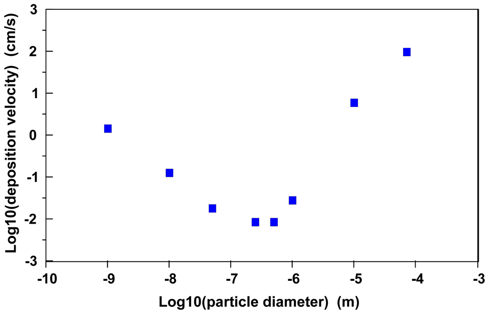
Figure 1 illustrates predicted average air/surface particle atmospheric deposition velocities as a function of particle diameter for particles with a net density of 10 g/cm³ [33]. As this is a fairly high density material, gravitational and impaction processes are likely to be more significant with these particles than would be observed with similarly sized materials of lesser density.

The rightmost portion of the curve in Figure 1 illustrates the effects of gravitational settling and impaction on predicted deposition velocities. Essentially, particles with a diameter much greater than 1 μm approach a deposition velocity equal to the terminal settling velocity for a mass in the atmosphere. The minimum predicted deposition velocities are for particles in the size range 0.1 μm to 1 μm; presumably particles in this size range would exhibit the greatest atmospheric transport. Because of this phenomenon, Hoffman [32] estimates that particles in the 0.1 μm to 1.0 μm size range also are less likely to deposit in the human respiratory system.

The descending portion of the curve on the left side of Figure 1 illustrates the transition to a particle size range where the deposition velocity is largely dominated by diffusive transport across a thin, laminar, stagnant layer in the interfacial region. Equation (3) can be rearranged to define a deposition velocity (v_d) governed by diffusive processes:

If one has paired experimental measurements of the deposition flux [F; g/(cm²s)] and the concentration gradient dC (where dC = g/cm³ _atm–g/cm³ _srf) or the diffusivity and the thin stagnant layer thickness, one can estimate a deposition velocity (v_d) in units of cm/s (e.g., [27]). In addition, if the rate of surface to air transport is insignificant or the initial concentration in the surface region is zero, then one also can simplify dC to equal the atmospheric concentration (g/cm³ _atm—[30,33,34]). Given the diffusivity estimates in Table 1, one also may estimate particle diffusion-limited deposition velocities provided that one has an estimate of the thickness of the thin stagnant layer dz [30].

The leftmost portion of the curve in Figure 1 illustrates that nanoparticle diffusivities become a major variable in predicting atmospheric air/surface deposition velocities. Essentially, maximum deposition velocities will be exhibited by gases in the diffusion-limited regime and minimal deposition velocities will occur with particles in a diameter size range of 0.1 μm to 1 μm.

In the case of air/water deposition, a situation may arise whereby one may have turbulent mixing in both the overlying atmospheric air mass and the underlying water body. In this situation, two thin, diffusive layers may limit intermedium exchange [35,36]) and one therefore needs diffusivities in both media and thicknesses of the two respective diffusive thin layers. Gladyshev [37] suggests that the thin stagnant aqueous layer at the air/water interface may range from 0.01 mm to 0.15 mm for gaseous oxygen exchange.

Traditional fate and transport modelers generally rely on partition coefficients (K_ds; where K_d = C_solid/C_water) to simulate potential toxicant transport and biological exposures in natural waters. For nonpolar uncharged chemicals, it is frequently assumed that partitioning occurs through binding with natural organic matter (NOM) and the associated organic carbon partition coefficients (K_ocs) can be related to experimentally measured octanol-water partition coefficients (K_ows) with a variety of regression relationships [36]. Ionizable toxicants are far more problematic; however, empirically derived partition coefficients for ionizable species also find utility in the fate, transport and exposure modeling community [20].

The fundamental theoretical interpretation of a partition coefficient (K_d) is that equilibrium partitioning occurs: (1) when the chemical potential of the species of interest is the same in both phases; and/or (2) when forward and backward rates of intermedium exchange are equal. As the rate for attaining equilibrium is diffusion limited, the 4 to 13 day equilibration period reported by Jafvert and Kulkarni [21] for the smallest of MNs may represent the minimum required equilibration period for MNs possessing larger dimensions.

Given the limitations of equilibrium partitioning theory for larger MNs in water, classical colloid chemistry may address the issue of colloidal suspension stability with the Derjaguin-Landau-Verwey-Overbeek (DLVO) theory (developed in the 1940s [38]). According to DLVO theory, particles in aqueous suspension experience two opposing energies: (1) attractive energies resulting from London/Van der Waals/Keesom dipole interaction energies; and (2) repulsive electrostatic energies that occur when two electrostatically like-charged particles in water approach one another. In situations where the repulsive electrostatic energies dominate, the suspension remains stable in water. In situations where the electrostatic repulsive energies are minimized such that the attractive energies can dominate, the particles are likely to aggregate, settle out and become immobile. The two variables commonly used to quantify these opposing energies are Hamaker constants (for attractive energies; [39–41]) and zeta potentials (for repulsive energies; [42,43]).

Traditional DLVO theory can be extended through either the adoption of additional non-DLVO energies and/or describing the interaction between particles and dissimilar (environmental) surfaces. Extending DLVO theory requires incorporating one or more additional parameters with their associated uncertainties. Using DLVO theory to interpret interactions between suspended particles and chemically dissimilar environmental surfaces requires knowledge of parameters that is not commonly available (and hence limits the utility of this approach). For these reasons, an approach examining the usefulness (and associated uncertainties) of traditional DLVO theory for making predictions of the likely self-aggregation behavior of colloidal suspensions is currently under investigation [14,15, and the present work].

Hamaker constants are required in DLVO theory. Typically, Hamaker constants for colloidal particles in water range from ~10⁻¹⁹ J (for aluminum and iron oxides) to ~10⁻²¹ J (for some biocolloids). The comparatively large Hamaker constants associated with aluminum and iron oxides help explain why solutions of alum and ferric chloride are commonly used to clarify turbid water samples. The relatively low Hamaker constants frequently observed with biocolloids explains both why biocolloids are sometimes observed in aged natural waters and why erstwhile unstable suspensions remain in aqueous suspension as the result of natural organic matter coatings that may dominate the interfacial properties of the suspended particles.

The understanding of interfacial properties as it relates to estimating zeta potentials is an active area of research. Generally speaking, zeta potentials can be estimated from electrokinetic experimental data [24,42,43] or they can be related to diffuse layer potentials estimated with geochemical speciation models (e.g., Diffuse Layer models [44], Triple Layer models [45]). The zeta potential is understood to be the potential at the “plane of shear” that is located a distance away from the beginning of the diffuse layer and is therefore generally considered have a magnitude that either equals or is less than that of the diffuse layer potential [42,43,45,46].

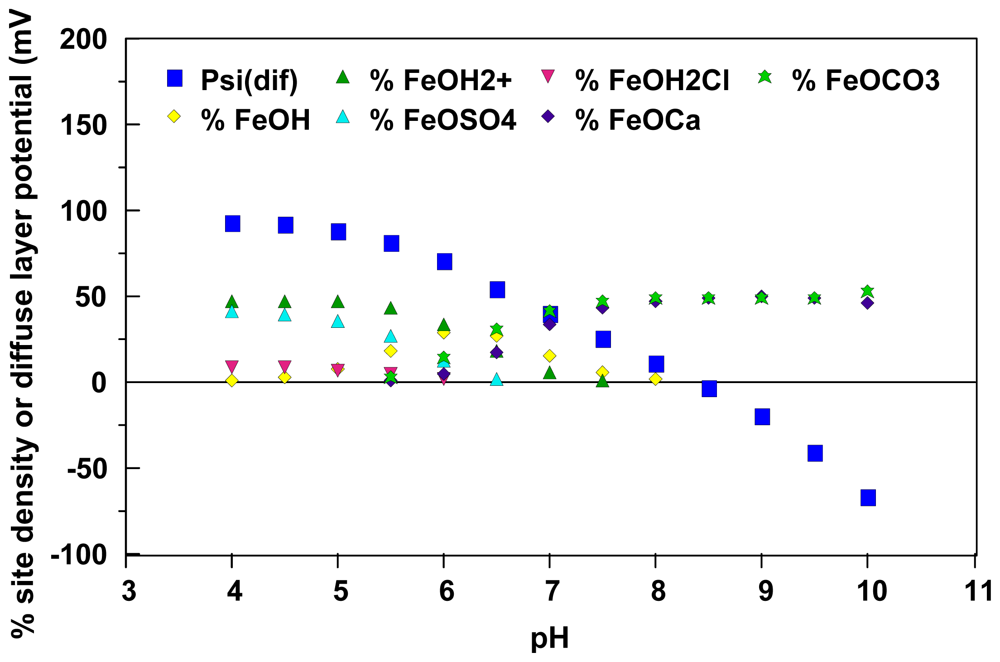
Figure 2 provides mechanistic insight into the observations reported by Degueldre et al. [13] that water chemistry can play a major role in the likely stability of aqueous colloidal suspensions. This figure illustrates both simulated diffuse layer potentials and the relative site distributions of ionizable sites on the surface of colloidal amorphous iron oxide particles suspended in “world average river water” as a function of pH [15]. These simulations were conducted using an enhanced version [15] of the MIT Diffuse Layer Model [44] that is currently in the MINTEQA2 geochemical speciation model [47]. From these simulations, surficial iron oxide sites are likely to be dominated by doubly protonated sites and surface complexed sulfate ions at low pH conditions and are likely to be dominated by surface sites that are complexed with calcium and carbonate ions at high pH conditions. As illustrated in the figure, surface complexation with the ions commonly found in water also can have a significant impact on model-generated diffuse layer potential estimates. In turn, these diffuse layer potential estimates can be interpreted as representing the maximum magnitude of the possible zeta potentials for amorphous iron oxide particles under these conditions.

If one has estimates of both Hamaker constants (from experimental data) and zeta/diffuse layer potentials (either experimentally measured or obtained from electrostatic surface complexation models) for a given colloidal suspension in water, one can make predictions as to whether or not that colloidal suspension will rapidly aggregate in natural waters. Basically, under conditions where the energies of attraction equal and counterbalance the energies of repulsion with distance from the particle surface, mathematically one can define a Critical Coagulation Concentration (CCC). The critical coagulation concentration is the minimum dissolved salt content (or ionic strength I-- I = 1/2∑c_iz_i ²; where c_i is the concentration of ions of valence z_i) needed to lead to the rapid aggregation of a suspension in water. Although like-charged particles in aqueous suspension will experience electrostatic repulsion, the presence of higher dissolved salt concentrations will lead to a partial screening of these electrostatic repulsive energies when ions of opposite charge accumulate between the particles. This ionic strength sensitivity explains the observation that suspended colloidal particles in freshwater rivers may well aggregate once the river water discharges into higher ionic strength estuaries.

Three published room temperature expressions for estimating CCCs at room temperature include [48–50]:

[48]

[49]

[50]

where following traditional colloid chemistry, the variables in equations (5) through (7) are defined by: γ = (EXP(zeΨ/2kT) − 1)/(EXP(zeΨ/2kT) + 1, not to be confused with the interfacial tension given in Equations (1) and (2). Ψ is the zeta potential [V], k is the Boltzmann constant [J/K], T is the absolute temperature [K], e is the charge of the proton [C], z is the counterion valence, and A is the Hamaker constant [J]. These expressions were used to estimate the potential self-aggregation behavior of a number of metal oxide suspensions in water; additional assumptions employed in developing these expressions are discussed in refs. [14,15].

Fowkes [51] published an expression for estimating room temperature critical interfacial potentials as functions of Hamaker constants. Fowkes defined his potential as a surface potential; in this work the requisite interfacial potential in Fowkes’ expression is assumed to be a zeta potential. Using these assumptions, a critical zeta potential can be defined as the minimum magnitude of the zeta potential needed to maintain a stable colloidal suspension in water. In SI units, Fowkes’ expression is:

where Ψ_crit is the magnitude of the minimum interfacial (zeta) potential required to maintain a stable suspension, A₁₂₁ is the Hamaker constant describing the attractive interactions between two particles of phase one in a liquid of phase two (water in this case) and 1/κ represents the ionic-strength-dependent Debye length. Fowkes developed this expression assuming that the attractive and repulsive energies counterbalanced one another when the two particles were a distance of 1/κ apart.

Using Equation (8) one can estimate amorphous iron oxide critical zeta potential values of ±24 mV to ±33 mV for the simulated world average river water data depicted in Figure 2. When one compares the diffuse layer potentials with these critical zeta potentials, it is suggested that maximum coagulation rates are likely to occur between pH values of ~7 to ~9. Johnson and Amirtharajah [52] suggested optimum settling conditions for amorphous iron oxide suspensions in a pH range of 6 to 10. Hence, these findings are consistent with previous observations [44,53,19] that the magnitude of the MIT diffuse layer model diffuse layer potential estimates likely exceed that of the associated zeta potentials (i.e., the shear plane is distant from the beginning of the diffuse layer).

The possibility also exists that “ballpark” estimates may be useful for screening-level assessments of the potential mobility of MNs in natural waters. For example, Sprycha [54] suggests that shear plane charge densities rarely exceed an absolute value of 0.02 C/m². Loux and Anderson [55] suggested that interfacial potentials in environmental aquatic systems are unlikely to exceed an absolute value of 25 mV (due to the ubiquity of multivalent ions in natural waters). Table 2 evaluates some of these “rule of thumb” assertions. Generally speaking, the assumption of a maximum diffuse layer charge density of 0.02 C/m² (with associated potential) or the assumption of a maximum diffuse layer potential of 25 mV would provide useful insight only at the highest ionic strengths where colloidal particles are already considered to likely aggregate. These observations support a contention that more sophisticated approaches will likely be required to assess MN mobility in environmental waters.

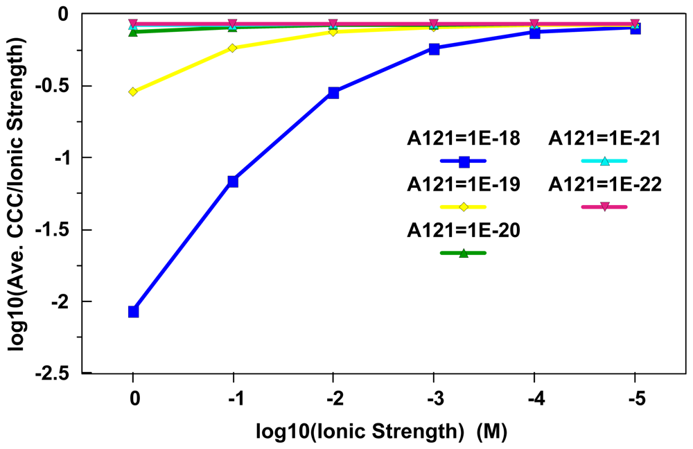
Figure 3 represents a test of consistency between the critical zeta potential concept given by Fowkes [51] and CCC Equation (6) [49]. Essentially, critical zeta potentials were estimated using Equation (6) over a Hamaker constant range of 1×10⁻¹⁸ J to 1×10⁻²² J at ionic strengths ranging from 1×10⁻⁵ M to 1 M. The representative critical zeta potential estimates, Hamaker constants and Debye layer thicknesses were then inserted into Equation (6) to estimate the CCC values needed to reach optimum aggregation rates. Ideal agreement between the two approaches would occur when the expression log₁₀(CCC/Ionic Strength) equals zero. It is perhaps fortuitous that MNs with the lowest Hamaker constants that are likely to be mobile at ionic strengths less than 0.01 M yield an agreement approaching 18% in these stability metrics under these conditions. If one performs a similar exercise with the averages of Equations (5)–(7), the minimum difference approaches 50%. Given that Ackler et al. [40] found that Hamaker constants may differ by as much as a factor of 7; these estimates suggest that experimental uncertainties may in some cases surpass the conceptual uncertainties in these comparisons.

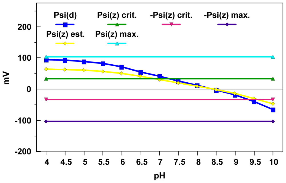
Figure 4 illustrates one approach for converting the diffuse layer potentials illustrated in Figure 2 into estimated zeta potentials (employing procedures delineated in Lyklema and Overbeek [46]). These calculation results are in accord with previous observations that the zeta potential can be significantly less than the diffuse layer potential at higher charge densities. It is well known from electrokinetic studies that zeta potentials typically reach maximum values for a given ionic strength; Lyklema and Overbeek [46] interpreted this phenomenon as resulting from changes in the aqueous viscosity as a function of field strength in the interfacial region.

Using procedures developed by these authors, one can estimate a maximum zeta potential magnitude for the world average river water simulations depicted in Figures 2 and 4 of ≈103 mV. This maximum zeta potential estimate does appear to agree reasonably well with the low pH diffuse layer potential estimates depicted in these figures. When one compares the critical zeta potential magnitude estimates of ≈33 mV obtained using Equation (8) with the zeta potential estimates in Figure 4, one can predict an optimum pH range for aggregation of 6.8 to 9.6. This represents a slight improvement over the range result of 7 to 9.5 given in ref. [15] with respect to capturing the optimum iron oxide pH aggregation range of 6 to 10 determined by Johnson and Amirthirajah [52].