
Critical Dynamics in Stratospheric Potential Energy Variations Prior to Significant (M > 6.7) Earthquakes

 , , ,
, , ,
Abstract
:1. Introduction
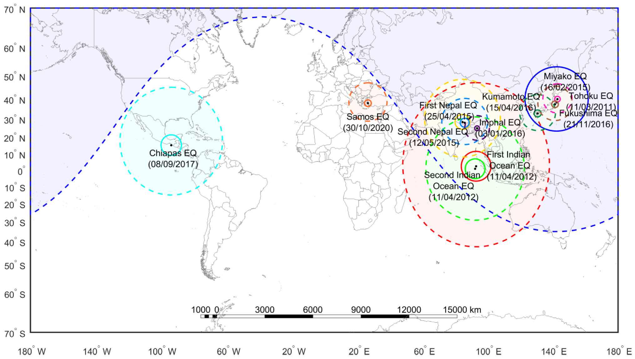
2. Studied EQs
3. Methods and Data
3.1. Computation of Potential Energy (EP) Using SABER/TIMED Temperature Profile
3.2. Natural Time (NT) Analysis Method
4. Analysis Results
5. Conclusions
Author Contributions
Funding
Data Availability Statement
Acknowledgments
Conflicts of Interest
References
- Hayakawa, M.; Molchanov, O.A. Seismo Electromagnetics: Lithosphere-Atmosphere-Ionosphere Coupling; TERRAPUB: Tokyo, Japan, 2002. [Google Scholar]
- Molchanov, O.A.; Hayakawa, M. Seismo Electromagnetics and Related Phenomena: History and Latest Results; TERRAPUB: Tokyo, Japan, 2008. [Google Scholar]
- Pulinets, S.; Ouzounov, D. Lithosphere–atmosphere–ionosphere coupling (LAIC) model—An unified concept for earthquake precursors validation. J. Asian Earth Sci. 2011, 41, 371–382. [Google Scholar] [CrossRef]
- Hayakawa, M. Earthquake Prediction with Radio Techniques; Wiley: Singapore, 2015. [Google Scholar]
- Eftaxias, K.; Potirakis, S.M.; Contoyiannis, Y. Four-Stage model of earthquake generation in terms of fracture-induced electromagnetic emissions a review. In Complexity of Seismic Time Series: Measurement and Application; Chelidze, T., Vallianatos, F., Telesca, L., Eds.; Elsevier: Oxford, UK, 2018; pp. 437–502. [Google Scholar]
- Potirakis, S.M.; Contoyiannis, Y.; Schekotov, A.; Eftaxias, K.; Hayakawa, M. Evidence of critical dynamics in various electromagnetic precursors. Eur. Phys. J. Spec. Top. 2021, 230, 151–177. [Google Scholar] [CrossRef]
- Uyeda, S.; Hayakawa, M.; Nagao, T.; Molchanov, O.; Hattori, K.; Orihara, Y.; Gotoh, K.; Akinaga, Y.; Tanaka, H. Electric and magnetic phenomena observed before the volcano-seismic activity in 2000 in the Izu Island Region, Japan. Proc. Natl. Acad. Sci. USA 2002, 99, 7352–7355. [Google Scholar] [CrossRef] [PubMed]
- Uyeda, S.; Nagao, T.; Kamogawa, M. Short-term earthquake prediction: Current status of seismo-electromagnetics. Tectonophysics 2009, 470, 205–213. [Google Scholar] [CrossRef]
- Uyeda, S. On earthquake prediction in Japan. Proc. Jpn. Acad. Ser. B 2013, 89, 391–400. [Google Scholar] [CrossRef] [PubMed]
- Varotsos, P.; Sarlis, N.V.; Skordas, E.S. Natural Time Analysis: The New View of Time Precursory Seismic Electric Signals, Earthquakes and Other Complex Time Series; Springer: Berlin, Germany, 2011. [Google Scholar]
- Hayakawa, M.; Izutsu, J.; Schekotov, A.; Yang, S.-S.; Solovieva, M.; Budilova, E. Lithosphere–atmosphere–ionosphere coupling effects based on multiparameter precursor observations for February–March 2021 earthquakes (M~7) in the offshore of Tohoku area of Japan. Geosciences 2021, 11, 481. [Google Scholar] [CrossRef]
- Sasmal, S.; Chowdhury, S.; Kundu, S.; Politis, D.Z.; Potirakis, S.M.; Balasis, G.; Hayakawa, M.; Chakrabarti, S.K. Pre-seismic irregularities during the 2020 Samos (Greece) earthquake (M = 6.9) as investigated from multi-parameter approach by ground and space-based techniques. Atmosphere 2021, 12, 1059. [Google Scholar] [CrossRef]
- Pulinets, S.; Ouzounov, D.; Davydenko, D.; Petrukhin, A. Multiparameter monitoring of short-term earthquake precursors and its physical basis. implementation in the Kamchatka Region. E3S Web Conf. 2016, 11, 00019. [Google Scholar] [CrossRef]
- De Santis, A.; Cianchini, G.; Marchetti, D.; Piscini, A.; Sabbagh, D.; Perrone, L.; Campuzano, S.A.; Inan, S. A multiparametric approach to study the preparation phase of the 2019 M7.1 Ridgecrest (California, United States) earthquake. Front. Earth Sci. 2020, 8, 540398. [Google Scholar] [CrossRef]
- Chetia, T.; Sharma, G.; Dey, C.; Raju, P.L. Multi-parametric approach for Earthquake Precursor Detection in assam valley (eastern Himalaya, India) using satellite and Ground Observation Data. Geotectonics 2020, 54, 83–96. [Google Scholar] [CrossRef]
- Piersanti, M.; Materassi, M.; Battiston, R.; Carbone, V.; Cicone, A.; D’Angelo, G.; Diego, P.; Ubertini, P. Magnetospheric–ionospheric–lithospheric coupling model. 1: Observations during the 5 August 2018 Bayan earthquake. Remote Sens. 2020, 12, 3299. [Google Scholar] [CrossRef]
- Hayakawa, M.; Schekotov, A.; Izutsu, J.; Nickolaenko, A.P. Seismogenic effects in ULF/ELF/VLF electromagnetic waves. Int. J. Electron. Appl. Res. 2019, 6, 1–86. [Google Scholar] [CrossRef]
- Phillips, O.M. On the generation of waves by turbulent wind. J. Fluid Mech. 1957, 2, 417. [Google Scholar] [CrossRef]
- Lighthill, J. Waves in Fluids; Cambridge University Press: Cambridge, UK, 2003. [Google Scholar]
- Fritts, D.C.; Alexander, M.J. Gravity wave dynamics and effects in the Middle Atmosphere. Rev. Geophys. 2003, 41. [Google Scholar] [CrossRef]
- Hayakawa, M.; Kasahara, Y.; Nakamura, T.; Hobara, Y.; Rozhnoi, A.; Solovieva, M.; Molchanov, O.; Korepanov, V. Atmospheric gravity waves as a possible candidate for seismo-ionospheric perturbations. J. Atmos. Electr. 2011, 31, 129–140. [Google Scholar] [CrossRef]
- Garmash, S.V.; Linkov, E.N.; Petrova, L.N.; Shved, G.N. Excitation of atmospheric oscillations by seismogravitational vibrations of the earth. Izv. Akad. Nauk. SSSR Fiz. Atmos. Okeana 1989, 35, 1290–1299. [Google Scholar]
- Linkov, E.M.; Petrova, L.N.; Zuroshvili, D.D. Seismogravitational vibrations of the earth and related disturbances of the atmosphere. Dokl. Akad. Nauk. SSSR 1989, 306, 315–317. [Google Scholar]
- Shalimov, S.L. Lithosphere-ionosphere relationship: A new way to predict earthquakes? Epis. Int. Geophys. Newsmag. 1992, 15, 252–254. [Google Scholar] [CrossRef]
- Miyaki, K.; Hayakawa, M.; Molchanov, O.A. The Role of Gravity Waves in the Lithosphere-Ionosphere Coupling, as Revealed from the Subionospheric LF Propagation Data. In Seismo-Electromagnetics: Lithosphere-Atmosphere-Ionosphere Coupling; Hayakawa, M., Molchanov, O., Eds.; TERRAPUB: Tokyo, Japan, 2002; pp. 229–232. [Google Scholar]
- Korepanov, V.; Hayakawa, M.; Yampolski, Y.; Lizunov, G. AGW as a seismo-ionospheric coupling responsible agent. Phys. Chem. Earth A/B/C 2009, 34, 485–495. [Google Scholar] [CrossRef]
- Nakamura, T.; Korepanov, V.; Kasahara, Y.; Hobara, Y.; Hayakawa, M. An evidence on the lithosphere-ionosphere coupling in terms of atmospheric gravity waves on the basis of a combined analysis of surface pressure, ionospheric perturbations and ground-based ULF Variations. J. Atmos. Electr. 2013, 33, 53–68. [Google Scholar] [CrossRef]
- Biswas, S.; Kundu, S.; Ghosh, S.; Chowdhury, S.; Yang, S.-S.; Hayakawa, M.; Chakraborty, S.K.; Chakrabarti, S.; Sasmal, S. Contaminated effect of geomagnetic storms on pre-seismic atmospheric and ionospheric anomalies during Imphal earthquake. Open J. Earthq. Res. 2020, 9, 383–402. [Google Scholar] [CrossRef]
- Kundu, S.; Chowdhury, S.; Ghosh, S.; Sasmal, S.; Politis, D.Z.; Potirakis, S.M.; Yang, S.-S.; Chakrabarti, S.K.; Hayakawa, M. Seismogenic anomalies in atmospheric gravity waves as observed from SABER/TIMED satellite during large earthquakes. J. Sens. 2022, 2022, 1–23. [Google Scholar] [CrossRef]
- Potirakis, S.M.; Schekotov, A.; Asano, T.; Hayakawa, M. Natural time analysis on the ultra-low frequency magnetic field variations prior to the 2016 Kumamoto (Japan) earthquakes. J. Asian Earth Sci. 2018, 154, 419–427. [Google Scholar] [CrossRef]
- Potirakis, S.M.; Schekotov, A.; Contoyiannis, Y.; Balasis, G.; Koulouras, G.; Melis, N.; Boutsi, A.; Hayakawa, M.; Eftaxias, K.; Nomicos, C. On possible electromagnetic precursors to a significant earthquake (MW = 6.3) occurred in Lesvos (Greece) on 12 June 2017. Entropy 2019, 21, 241. [Google Scholar] [CrossRef]
- Potirakis, S.M.; Karadimitrakis, A.; Eftaxias, K. Natural time analysis of critical phenomena: The case of pre-fracture electromagnetic emissions. Chaos 2013, 23, 023117. [Google Scholar] [CrossRef]
- Potirakis, S.M.; Contoyiannis, Y.; Asano, T.; Hayakawa, M. Intermittency-induced criticality in the lower ionosphere prior to the 2016 Kumamoto earthquakes as embedded in the VLF propagation data observed at multiple stations. Tectonophysics 2018, 722, 422–431. [Google Scholar] [CrossRef]
- Politis, D.Z.; Potirakis, S.M.; Contoyiannis, Y.F.; Biswas, S.; Sasmal, S.; Hayakawa, M. Statistical and criticality analysis of the lower ionosphere prior to the 30 October 2020 Samos (Greece) earthquake (M6.9), based on VLF electromagnetic propagation data as recorded by a new VLF/LF receiver installed in Athens (Greece). Entropy 2021, 23, 676. [Google Scholar] [CrossRef]
- Potirakis, S.M.; Contoyiannis, Y.; Melis, N.S.; Kopanas, J.; Antonopoulos, G.; Balasis, G.; Kontoes, C.; Nomicos, C.; Eftaxias, K. Recent seismic activity at Cephalonia (Greece): A study through candidate electromagnetic precursors in terms of non-linear dynamics. Nonlinear Process. Geophys. 2016, 23, 223–240. [Google Scholar] [CrossRef]
- Hayakawa, M.; Schekotov, A.; Potirakis, S.M.; Eftaxias, K. Criticality features in ULF Magnetic Fields prior to the 2011 Tohoku earthquake. Proc. Jpn. Acad. Ser. B 2015, 91, 25–30. [Google Scholar] [CrossRef]
- Ghosh, S.; Chowdhury, S.; Kundu, S.; Sasmal, S.; Politis, D.Z.; Potirakis, S.M.; Hayakawa, M.; Chakraborty, S.; Chakrabarti, S.K. Unusual surface latent heat flux variations and their critical dynamics revealed before strong earthquakes. Entropy 2022, 24, 23. [Google Scholar] [CrossRef]
- Dobrovolsky, I.P.; Zubkov, S.I.; Miachkin, V.I. Estimation of the size of earthquake preparation zones. Pure Appl. Geophys. 1979, 117, 1025–1044. [Google Scholar] [CrossRef]
- Bowman, D.D.; Ouillon, G.; Sammis, C.G.; Sornette, A.; Sornette, D. An observational test of the critical earthquake concept. J. Geophys. Res. Solid Earth 1998, 103, 24359–24372. [Google Scholar] [CrossRef] [Green Version]
- Shuai, J.; Zhang, S.D.; Huang, C.M.; Yi, F.; Huang, K.M.; Gan, Q.; Gong, Y. Climatology of global gravity wave activity and dissipation revealed by Saber/Timed Temperature Observations. China Technol. Sci. 2014, 57, 998–1009. [Google Scholar] [CrossRef]
- Remsberg, E.E.; Marshall, B.T.; Garcia-Comas, M.; Krueger, D.; Lingenfelser, G.S.; Martin-Torres, J.; Mlynczak, M.G.; Russell, J.M.; Smith, A.K.; Zhao, Y.; et al. Assessment of the quality of the version 1.07 temperature-versus-pressure profiles of the middle atmosphere from timed/saber. J. Geophys. Res. Atmos. 2008, 113, D17. [Google Scholar] [CrossRef]
- Yan, X.; Arnold, N.; Remedios, J. Global observations of gravity waves from high resolution dynamics limb sounder temperature measurements: A year long record of temperature amplitude and vertical wavelength. J. Geophys. Res. Atmos. 2010, 115, D10. [Google Scholar] [CrossRef]
- Yamashita, C.; England, S.L.; Immel, T.J.; Chang, L.C. Gravity wave variations during elevated stratopause events using SABER Observations. J. Geophys. Res. Atmos. 2013, 118, 5287–5303. [Google Scholar] [CrossRef]
- Thurairajah, B.; Bailey, S.M.; Cullens, C.Y.; Hervig, M.E.; Russell, J.M. Gravity Wave activity during recent stratospheric sudden warming events from Sofie Temperature Measurements. J. Geophys. Res. Atmos. 2014, 119, 8091–8103. [Google Scholar] [CrossRef]
- Yang, S.-S.; Hayakawa, M. Gravity wave activity in the stratosphere before the 2011 Tohoku earthquake as the mechanism of lithosphere-atmosphere-ionosphere coupling. Entropy 2020, 22, 110. [Google Scholar] [CrossRef]
- Varotsos, P.A.; Sarlis, N.V.; Skordas, E.S. Long-range correlations in the electric signals that precede rupture. Phys. Rev. E 2002, 66, 011902. [Google Scholar] [CrossRef]
- Varotsos, P.A.; Sarlis, N.V.; Tanaka, H.K.; Skordas, E.S. Similarity of fluctuations in correlated systems: The case of Seismicity. Phys. Rev. E 2005, 72, 041103. [Google Scholar] [CrossRef]
- Varotsos, P.A.; Sarlis, N.V.; Skordas, E.S. Spatio-temporal complexity aspects on the interrelation between seismic electric signals and seismicity. Pract. Athens Acad. 2001, 76, 294–321. [Google Scholar]
- Abe, S.; Sarlis, N.V.; Skordas, E.S.; Tanaka, H.K.; Varotsos, P.A. Origin of the usefulness of the natural-time representation of complex time series. Phys. Rev. Lett. 2005, 94, 170601. [Google Scholar] [CrossRef]
- Baldoumas, G.; Peschos, D.; Tatsis, G.; Chronopoulos, S.K.; Christofilakis, V.; Kostarakis, P.; Varotsos, P.; Sarlis, N.V.; Skordas, E.S.; Bechlioulis, A.; et al. A prototype photoplethysmography electronic device that distinguishes congestive heart failure from healthy individuals by applying natural time analysis. Electronics 2019, 8, 1288. [Google Scholar] [CrossRef] [Green Version]
- Varotsos, P.A.; Sarlis, N.V.; Skordas, E.S.; Nagao, T.; Kamogawa, M. The unusual case of the ultra-deep 2015 Ogasawara earthquake (Mw 7.9): Natural Time Analysis. EPL 2021, 135, 49002. [Google Scholar] [CrossRef]
- Sarlis, N.V.; Skordas, E.S.; Varotsos, P.A. A remarkable change of the entropy of seismicity in natural time under time reversal before the super-giant M9 Tohoku earthquake on 11 March 2011. EPL 2018, 124, 29001. [Google Scholar] [CrossRef]
- Hayakawa, M.; Potirakis, S.M.; Saito, Y. Possible relation of air ion density anomalies with earthquakes and the associated precursory ionospheric perturbations: An analysis in terms of criticality. Int. J. Electron. Appl. Res. 2018, 5, 56–75. [Google Scholar] [CrossRef]
- Yang, S.-S.; Potirakis, S.M.; Sasmal, S.; Hayakawa, M. Natural Time Analysis of global navigation satellite system surface deformation: The case of the 2016 Kumamoto earthquakes. Entropy 2020, 22, 674. [Google Scholar] [CrossRef]
- Varotsos, P.A.; Sarlis, N.V.; Skordas, E.S.; Tanaka, H.K.; Lazaridou, M.S. Entropy of seismic electric signals: Analysis in natural time under time reversal. Phys. Rev. E 2006, 73, 031114. [Google Scholar] [CrossRef]
- Sarlis, N.V.; Skordas, E.S.; Varotsos, P.A. Similarity of fluctuations in systems exhibiting self-organized criticality. EPL 2011, 96, 28006. [Google Scholar] [CrossRef]
- Potirakis, S.M.; Contoyiannis, Y.; Schekotov, A.; Asano, T.; Hayakawa, M. Analysis of the ultra-low frequency magnetic field fluctuations prior to the 2016 Kumamoto (Japan) earthquakes in terms of the method of critical fluctuations. Physica A Stat. Mech. Appl. 2019, 514, 563–572. [Google Scholar] [CrossRef]
- Contoyiannis, Y.; Potirakis, S.M.; Eftaxias, K.; Hayakawa, M.; Schekotov, A. Intermittent criticality revealed in ULF Magnetic Fields prior to the 11 march 2011 Tohoku earthquake (Mw = 9). Physica A Stat. Mech. Appl. 2016, 452, 19–28. [Google Scholar] [CrossRef]
- Potirakis, S.M.; Asano, T.; Hayakawa, M. Criticality analysis of the lower ionosphere perturbations prior to the 2016 Kumamoto (Japan) earthquakes as based on VLF electromagnetic wave propagation data observed at multiple stations. Entropy 2018, 20, 199. [Google Scholar] [CrossRef] [Green Version]


| Date | Time (UT) | Depth (km) | Epicenter Latitude | Epicenter Longitude | Magnitude (MW) | EQ Class | EPZ Radius (km) | CZ Radius (km) | Epicenter Location | Country/ Region |
|---|---|---|---|---|---|---|---|---|---|---|
| 11 March 2011 | 05:46:24 | 29 | 38.297° N | 142.373° E | 9.1 | Great | 8185 | 1674.9 | Tohoku * | Japan |
| 11 April 2012 | 08:38:36 | 20 | 2.327° N | 93.063° E | 8.6 | Great | 4989 | 1009.3 | Indian Ocean−1 * | Indo-Australian Plate |
| 11 April 2012 | 10:43:10 | 25.1 | 0.802° N | 92.463° E | 8.2 | Great | 3357 | 672.9 | Indian Ocean−2 * | Indo-Australian Plate |
| 16 February 2015 | 23:06:28 | 23 | 39.856° N | 142.881° E | 6.7 | Strong | 760 | 147.2 | Miyako | Japan |
| 25 April 2015 | 06:11:25 | 8.2 | 28.231° N | 84.731° E | 7.8 | Major | 2259 | 448.7 | Gorkha−1 * | Nepal |
| 12 May 2015 | 07:05:19 | 15 | 27.809° N | 86.066° E | 7.3 | Major | 1377 | 270.3 | Gorkha−2 * | Nepal |
| 15 April 2016 | 16:25:06 | 10 | 32.791° N | 130.754° E | 7.0 | Major | 1023 | 199.5 | Kumamoto * | Japan |
| 21 November 2016 | 20:59:49 | 9 | 37.393° N | 141.387° E | 6.9 | Strong | 936 | 180.3 | Fukushima | Japan |
| 3 January 2016 | 23:05:22 | 55 | 24.804° N | 93.651° E | 6.7 | Strong | 760 | 147.2 | Imphal ** | India |
| 8 September 2017 | 04:49:19 | 47.4 | 15.022° N | 93.899° W | 8.2 | Great | 3357 | 672.9 | Chiapas * | Mexico |
| 30 October 2020 | 11:51:27 | 21 | 37.897° N | 26.784° E | 7.0 | Major | 1023 | 199.5 | Samos *** | Greece |
| EQ Name and Magnitude (MW) | EP Enhancement Time (No. of Days before the EQ) | Maximum EP Altitude/ Altitude Range (km) | Analyzed Altitude Range |
|---|---|---|---|
| Tohoku * (9.1) | 4–6 | 43 | min: 42.040 km step: 0.067 km max: 44.050 km |
| Indian Ocean−1 & Indian Ocean−2 * (8.6 & 8.2) | 2–6 | 34–37 | min: 32.007 km step: 0.067 km max: 38.037 km |
| Miyako (6.7) | 9–11 | 38–42 | min: 38.027 km step: 0.067 km max: 41.779 km |
| Gorkha−1 * (7.8) | 13–14 | 35–36 | min: 33.000 km step: 0.067 km max: 37.087 km |
| Gorkha−2 * (7.3) | 1–3 | 34–36 | min: 33.010 km step: 0.067 km max: 37.432 km |
| Kumamoto * (7.0) | 8–9 | 43 | min: 40.033 km step: 0.067 km max: 44.99 km |
| Fukushima (6.9) | 2–4 | 44–46 | min: 41.037 km step: 0.067 km max: 45.995 km |
| Imphal ** (6.7) | 7–10 | 44–46 | min: 43.000 km step: 0.067 km max: 47.020 km |
| Chiapas * (8.2) | 7 | 42–46 | min: 41.037 km step: 0.067 km max: 45.995 km |
| Samos *** (7.0) | 5–7 | 46–48 | min: 45.117 km step: 0.067 km max: 49.539 km |
| EQ Name | Criticality Altitude (km) | Criticality Date (No. of Days before EQ) | Date of EQ Occurrence | Other Extreme Phenomena after the Occurrence of Criticality | Selected Time Period for the Analysis | Selected Spatial Region for the Analysis |
|---|---|---|---|---|---|---|
| Tohoku | 43.849–44.050 | 08 March 2011 (3) | 11 March 2011 | 17–23 March 2011 were disturbed due to three low pressure cyclonic systems | 15 February 2011– 21 March 2011 | (20°, 60°) N, (120°, 160°) E |
| Indian Ocean−1 & Indian Ocean−2 * | 32.007–34.486 | 07 April 2012 (4) | 11 April 2012 | A tropical low-pressure area of 19U was formed during 16–25 April 2012. Also, equatorial KWs. | 13 March 2012– 21 April 2012 | (–15°S, 10° N), (70°, 110°) E |
| Miyako | 38.228, 38.429, 38.764, 39.769, 39.836, 39.903, 39.970, 40.037, 40.104, 40.171, 40.707, 41.042, 41.779 | 07 February 2015– 13 February 2015 (3–9) | 16 February 2015 | - | 17 January 2015– 26 February 2015 | (25°, 50°) N, (130°, 160°) E |
| Gorkha−1 | 33.000, 33.067, 33.268, 33.469, 33.938, 34.407, 35.010, 35.144, 35.613, 36.082, 36.484, 36.752, 37.087 | 15 April 2015–24 April 2015 (1–10) | 25 April 2015 | - | 10 April 2015– 20 April 2015 | (20°, 40°)N, (70°, 110°)E |
| Gorkha−2 | 33.010, 33.268, 33.814, 35.556, 35.958, 36.360, 36.762, 37.030, 37.432 | 26 April 2015–4 May 2015, (8–16) | 12 May 2015 | - | 10 April 2015– 20 May 2015 | (20°, 40°)N, (70°, 110°)E |
| Kumamoto | 40.033–40.435 | 06 April 2016–13 April 2016 (2–9) | 15 April 2016 | 14 April–19 March 2016 were disturbed due to a few frontal systems | 15 March 2016– 25 April 2016 | (15°, 40°)N, (120°, 140°)E |
| Fukushima | 41.908, 42.109, 42.176, 42.243, 42.980, 43.449, 43.516, 43.918, 45.660, 45.928, 45.995 | 12 November 2016–15 November 2016 (6–9) | 21 November 2016 | - | 21 October 2016– 01 December 2016 | (25°, 50°)N, (125°, 150°)E |
| Imphal | 43.000, 43.603, 44.206, 45.010, 45.479, 45.948, 46.484, 46.819 | 26 December 2015–29 December 2015 (5–8) | 03 January 2016 | - | 15 December 2016– 13 January 2016 | (15°, 35°)N, (70°, 110°)E |
| Chiapas | 45.660–45.995 | 29 August 2017 (10) | 08 September 2017 | Hurricane “Katia” (05–09 September 2017) in the region (22°, 25°)N, (94°, 98°)W Also, equatorial KWs | 08 August 2017– 18 September 2017 | (5° S, 25° N), (70°, 110°)W |
| Samos | - | - | 30 October 2020 | - | 30 September 2020– 30 November 2020 | (30°, 50°)N, (10°, 40°)E |
Publisher’s Note: MDPI stays neutral with regard to jurisdictional claims in published maps and institutional affiliations. |
© 2022 by the authors. Licensee MDPI, Basel, Switzerland. This article is an open access article distributed under the terms and conditions of the Creative Commons Attribution (CC BY) license (https://creativecommons.org/licenses/by/4.0/).
Share and Cite
Politis, D.Z.; Potirakis, S.M.; Kundu, S.; Chowdhury, S.; Sasmal, S.; Hayakawa, M. Critical Dynamics in Stratospheric Potential Energy Variations Prior to Significant (M > 6.7) Earthquakes. Symmetry 2022, 14, 1939. https://doi.org/10.3390/sym14091939
Politis DZ, Potirakis SM, Kundu S, Chowdhury S, Sasmal S, Hayakawa M. Critical Dynamics in Stratospheric Potential Energy Variations Prior to Significant (M > 6.7) Earthquakes. Symmetry. 2022; 14(9):1939. https://doi.org/10.3390/sym14091939
Chicago/Turabian StylePolitis, Dimitrios Z., Stelios M. Potirakis, Subrata Kundu, Swati Chowdhury, Sudipta Sasmal, and Masashi Hayakawa. 2022. "Critical Dynamics in Stratospheric Potential Energy Variations Prior to Significant (M > 6.7) Earthquakes" Symmetry 14, no. 9: 1939. https://doi.org/10.3390/sym14091939