Article

Friendship of Stock Market Indices: A Cluster-Based Investigation of Stock Markets

1
Department of Finance, Budapest University of Technology and Economics, Magyar tudosok krt. 2., 1117 Budapest, Hungary
2
Department of Economics, Janos Selye University, Hradná ul. 21., 94501 Komarno, Slovakia
*
Author to whom correspondence should be addressed.
J. Risk Financial Manag. 2018, 11(4), 88; https://doi.org/10.3390/jrfm11040088
Submission received: 3 November 2018 / Revised: 7 December 2018 / Accepted: 11 December 2018 / Published: 13 December 2018
(This article belongs to the Special Issue Mathematical Finance with Applications)

Abstract

:
This paper introduces a spectral clustering-based method to show that stock prices contain not only firm but also network-level information. We cluster different stock indices and reconstruct the equity index graph from historical daily closing prices. We show that tail events have a minor effect on the equity index structure. Moreover, covariance and Shannon entropy do not provide enough information about the network. However, Gaussian clusters can explain a substantial part of the total variance. In addition, cluster-wise regressions provide significant and stationer results.

Graphical Abstract

1. Introduction

The global stock market structure has to be well understood to diversify risk and manage cross-border equity portfolios. Appropriate portfolio construction is rather complicated. The linear dependence structure of the network is not stable (Erdős et al. 2011; Song et al. 2011; Maldonado and Anthony 1981). Moreover, exogenous shocks have major impact on the correlation structure; hence, uncorrelated assets could start moving together (Heiberger 2014). Therefore, correlation-based techniques could cause unwanted variance peaks.
Institutional economic surveys (like MSCI 2018) provide qualitatively identified network structures e.g., emerging markets and developed markets to stabilize their classification.
The main goal of this study is to provide more suitable quantitative techniques, generalize the widely used correlation-based portfolio construction framework, discover the equity index network and make diversification reliable.
The baseline concept follows the Sharpe (1964) Capital Asset Pricing Model (CAPM), in which similarity measures are calculated from correlations between logarithmic returns (Yalamova 2009). The anomalies of CAPM indicate a two-dimensional mean-beta framework that gives only a simplified picture of the real market structure. In order to explain the residuals, financial variables appeared in the famous regression (Fama and French 1996).
In this paper, we carry out a graph theory-based approach to unveil embedded network level information (Shi and Malik 2000). We propose non-linear similarity kernels that are able to deal with higher-order terms. We introduce novel jump-based similarity to investigate the effect of shocks. In addition, we test whether relative entropy of the distribution functions, that captures non-Gaussian behavior, conveys network level information. We also investigate the widely used Gaussian smoothing and correlation (Luxburg 2007). We compare different spectral clustering techniques and introduce the usage of the normalized Newman–Girvan cut (Bolla 2011).
Analyzing historical data supports the a priori assumption that clusters are homogenously connected. Thus, normalized Laplacian based techniques (Takumasa 2015) are not applicable. However, the proposed Newman-Girvan cut brings suitable, stationary clustering results. We calculate correlation, jump, relative entropy and Gaussian-based similarities. The figures show that Newman–Girvan cut outperforms normalized Laplacian technique. Analyzing the spectral property of the jump-based similarity matrix unveils that exogenous shocks have minor effect on the network. Thus, our novel results imply that shocks do not convey sufficient information about the equity index graph. Regression analysis demonstrates the stationarity and explanatory power of the clusters. Moreover, we shed some light on the node level equity index structure. We unveil that the index network has scale free properties. Nevertheless, we show that geographical and qualitative categorizations are in line with clusters.
The article structured as follows: in Section 2 we introduce our spectral clustering-based concept. In Section 3 we analyze the equity index graph, compare different similarity matrices and clustering techniques. Section 4 summarizes the article.

2. Materials and Methods

2.1. Data

The current study presents a detailed analysis of 59 stock indices. We apply USD denominated stock splits and dividend-adjusted daily closing prices between 26 September 1990 and 21 September 2015; data is provided by Thomson Reuters.
Our selection criteria for covered stock indices is based on their classification in the International Monetary Fund (IMF) Economic Outlook 2015, and the MSCI WORLD Index composition in 2015. In our analysis we allocate approximately the same weight to each region, despite an unequal number of countries and market capitalization. We rebalance the sample by choosing approximately ten indices from each IMF group. We are also interested in the role of well diversified indices e.g., MSCI WORLD and EURO STOXX600, which have also been analyzed.
In order to underline the highly different characteristics of individual stock indices, we present some monthly descriptive statistics in Table 1.

2.2. Methodology

In the 20th Century, the appearance of large, complex data sets brought new challenges to developing methods which could be used to understand complicated structures. The key concept is to classify data points according to various similarity functions. The problem is computationally extremely challenging. However, spectral clustering techniques provide optimal, lower dimensional representation of multidimensional data sets. The idea is twofold: on the one hand, similarly to principal component analysis we could calculate lower dimensional representation of the data points from the eigenvalues and eigenvectors of the similarity matrix. On the other hand, we could represent the data structure as a weighted graph and cut the graph along the different clusters. This approach leads to penalized cut optimization problems. Linear algebra and cluster analysis provide powerful methods to find the optimal representations and minimized cuts.

2.2.1. Similarity Matrix

If we would like to cluster different items, first the measurement of similarity has to be decided. In this study similarity of two stock indices ( i , j ) will be denoted by W i , j . The goal is to penalize differences and reward similarities. Logarithmic returns are easy to handle and maintain all price process information.
r i ( t ) = ln ( S i ( t ) / S i ( t 1 ) ) ,
where S i ( t ) represents the price of index i . The current study analyses multiple similarity approaches.
First, the Markowitz-based squared correlation is considered a similarity metric.
W i , j = Corr 2 ( r i , r j ) ,
We argue this approach because logarithmic returns are not normally distributed, hence non-linear effects may also be important. However, as correlation is linear, squared correlation similarities only take into account linear dependences.
The problem of higher-order moments can be easily solved by using symmetric and positive-definite kernel functions. The idea comes from the functional analysis. Data can be transformed into a reproducing kernel Hilbert space (RKHS), where applying the usual statistics provides the same outcomes as can be attained by using non-linear statistics in the original Hilbert space (Berlinet and Christine 2011); and, in practice, the Gaussian-kernel is widely used (Leibon et al. 2008).
W i , j = exp ( r i r j 2 ) ,
We notice that, if the sets of the relevant information and sensitivities are similar, then the relative entropy of the distribution of return processes is small. Otherwise, we can say stock indices are sensitive to different sets of information in a different manner (Ormos and Zibriczky 2014). This means that the similarity function has to be monotonically decreasing in symmetric Kullback–Leibler distance, and so we can construct a similarity measure such that:
W i , j = 2 / ( 2 + [ KL ( p ( r i ) p ( r j ) ) + KL ( p ( r j ) p ( r i ) ) ] ) ,
where p ( r i ) denotes the probability distribution function of logarithmic returns of index i and KL ( p ( r i ) p ( r j ) ) = def p ( r i = x ) ln ( p ( r i = x ) / p ( r j = x ) ) the relative entropy of indices i and j.
Another perspective argues that large deviations are riskier, hence similarities should be defined with tail distributions. We calculate the differences of the return series and count the number of at least two standard deviation peaks. This logic implies that indices are similar if their price processes jump together. Similarity function has to be decreasing in the number of large deviations, hence we propose the following metric:
W i , j = 1 / ( 1 + t = 1 T δ ( |   z i ( t ) z j ( t ) | > 2 ) ) ,
where z i represents the normalized return of index i .
In the current study we compare each approach.

2.2.2. Normalized Modularity

The equity index structure is strongly connected. We cannot say that events in Africa do not have any effect on European markets, hence we have to find methods which can be used to cluster dense graphs.
Let G ( V N × 1 , W N × N ) be a weighted graph, where V denotes the set of vertices and W represents the weights of the edges. A k-partition of graph G ( V , W ) can be defined as the partition of vertices such that a = 1 k V a = V and V i V j = δ i , j V i ,   i , j { 1 , , k } .
The W i , j value represents the strength of the connection between nodes ( i , j ) . If we assume that nodes are independently connected, then the guess of weight W i , j will be the product of the average connection strength of i and j. The average connection strength d i and d j are given by W ,
d i = 1 N u = 1 N W i , u ,
Thus, W i , j d i d j captures the information of the network structure (Bolla 2011). If we want to maximize the sum of information in each cluster, we get:
max P k P k a = 1 k i , j V a ( W i , j d i d j ) ,
where P k stands for specific k-partition in P k , which represents the set of all possible k-partitions.
Let M : = W d d T denotes the modularity matrix of G ( V , W ) . If we would like to get clusters with similar volumes, then we have to add a penalty to Equation (6), hence we get the normalized Newman–Girvan cut.
max P k P k a = 1 k 1 Vol ( V a ) i , j V a ( W i , j d i d j ) ,
where Vol ( V a ) = u V a d u .
Let us define the so called normalized modularity matrix:
M D : = D 1 / 2 M D 1 / 2 ,
If we would like to cluster a weighted graph G ( V , W ) , then eigenvectors of its modularity ( M ) and normalized modularity matrices ( M D ) can be used. Modularity and normalized modularity matrices are symmetric and 0 is always in the spectrum of M D :
M D = i = 1 N λ i u i = i = 1 N 1 λ i u i ,
where 1 > λ 1 λ 2 λ N 1 denote the eigenvalues of M D .
If we would like to maximize Equation (7), then we can use the k-means clustering algorithm on the optimal k-dimensional representation of vertices,
( D 1 2 u 1 , , D 1 2 u k ) T ,
where u 1 , , u k denote the corresponding eigenvalues of | λ 1 ( M D ) | | λ k ( M D ) | . Moreover, if the normalized modularity matrix has large positive eigenvalues, then the graph has well-separated clusters, otherwise clusters are strongly connected.
Another natural approach is to minimize the normalized cut (Luxburg 2007).
m i n P k P k a = 1 , b = a + 1 k 1 , k ( 1 Vol ( V a ) + 1 Vol ( V b ) ) W i , j ,
The optimization problem is similar to Equation (7). However, instead of the normalized-modularity matrix the normalized Laplace matrix provides the solution (Shi and Malik 2000).
L D : = D 1 2 ( D W ) D 1 2 ,
This technique works when clusters are well separated, otherwise normalized modularity gives better results.

2.2.3. Algorithm

In empirical analysis, the following steps are the backbone of the calculation (Filippone et al. 2007).
  • Constructing the similarity matrix ( W ) .
  • Calculating the normalized modularity matrix ( M D ) .
  • Based on the spectral gap, determining the number of clusters and optimal k-dimensional representation.
  • Appling k-means clustering.

2.2.4. Assessment of Clustering Methods

The relevance of different clustering techniques can be tested in multiple ways. The most common metrics follow a regression-based logic. In this framework we suppose that variance has two components: the within, and the between cluster components. Therefore, the explanatory power of given clusters can be described as:
j = 1 k j = 1 N i ( X i , j X ¯ ) 2     i = 1 k j = 1 N i ( X i , j X i ¯ ) 2 i , j = 1 N i ,   N j ( X i , j X ¯ ) 2 ,
where k represents the number of clusters, N i shows the size of clusters and X ¯ , X ¯ i stands for the total and cluster wise average (Zhao 2012). The formula penalizes dispersions within clusters, hence dense clusters would give a number close to 1 . Moreover, calculating the ratios with a different number of clusters highlights the optimal number of clusters.

3. Results

This study presents a broad analysis of the equity index network structure. Logarithmic returns of 59 stock indices are clustered in different ways. Our investigations reveal stock indices are homogenously connected, and large price changes have limited effect on the network structure.

3.1. Similarity Metrics

Defining similarity is a key aspect in clustering. In general, it is not usually possible to find an optimal kernel, but different approaches can be tested and compared to specific data sets.
This study analyzes correlation, jump, entropy, and Gaussian-based similarity kernels. When calculating the similarity matrices, we expect strongly connected indices have coefficients close to one, whereas loosely connected close to zero. Level plots (Figure 1) give a feeling about the network structure which seems to be homogeneous; thus, clusters could not be well separated.
Figure 1 displays the correlation, Gaussian-kernel, relative entropy and jump-based similarity structure of the equity index graph, in which the whiter the color the stronger the connection between the indices. Indices are sorted alphabetically and ( i , j ) represents the similarity between index i and j .
Different similarity measures imply similar patterns, which is in line with our a priori intuition. However, the spectra of normalized Laplace and normalized modularity matrices help us to find the most adequate kernel function: the wider the spectral gap, the better the clustering property. This means, we have to find similarity metrics, which in turn implies large gaps in the spectrum of normalized Laplacian and modularity matrix (Chung 1997).
Empirical evidences (Figure 2 and Figure 3) show relative entropy, and Gaussian-kernel can also be used to cluster the stock index network while correlation and jump-based similarities are not promising.
A correlation-based similarity approach implies roughly uniform eigenvalue density on [ 0 ,   1 ] . This means, a lot of gaps appear in the spectrum, hence we could not comment on the optimal number of clusters. Moreover, lower dimensional representations will not contain all the information as some of the large eigenvalues are not considered. These hurdles highlight the problems of squared correlation similarity matrices.
Counting at least two standard deviation jumps results in a small number of eigenvalues with large multiplicity. Therefore, lower dimension representation cannot be used to cluster the data points. Accordingly, jumps are random and do not reflect the network structure; thus we could say all the clusters are exposed to the same systematic risk. Thus, the results provide evidence of spillover effect. Moreover, we show that shocks and market collapses have a minor effect on the equity index graph i.e., network structure of equity indices.
Gaussian and relative entropy-based similarity matrices infer promising figures, especially in the case of normalized modularity. Here, we get large well separated eigenvalues necessary to transform the data into a lower dimensional space.
Notice that these results are in line with Figure 1 because the normalized Laplacian minimizes the normalized cut (Equation (10)), which in turn, is small if, and only if, the clusters are loosely connected. Whereas, the modularity approach maximizes the information of clustering, hence, it can also be used in a homogeneous network structure as well.
Investigating the spectra, especially the positions of spectral gaps, gives some guidance on the optimal number of clusters. Considering the previous results, the spectra of Gaussian and relative entropy-based normalized modularity matrices are suitable. Figure 4 shows indices could be put into 2, 3, or 5 clusters.
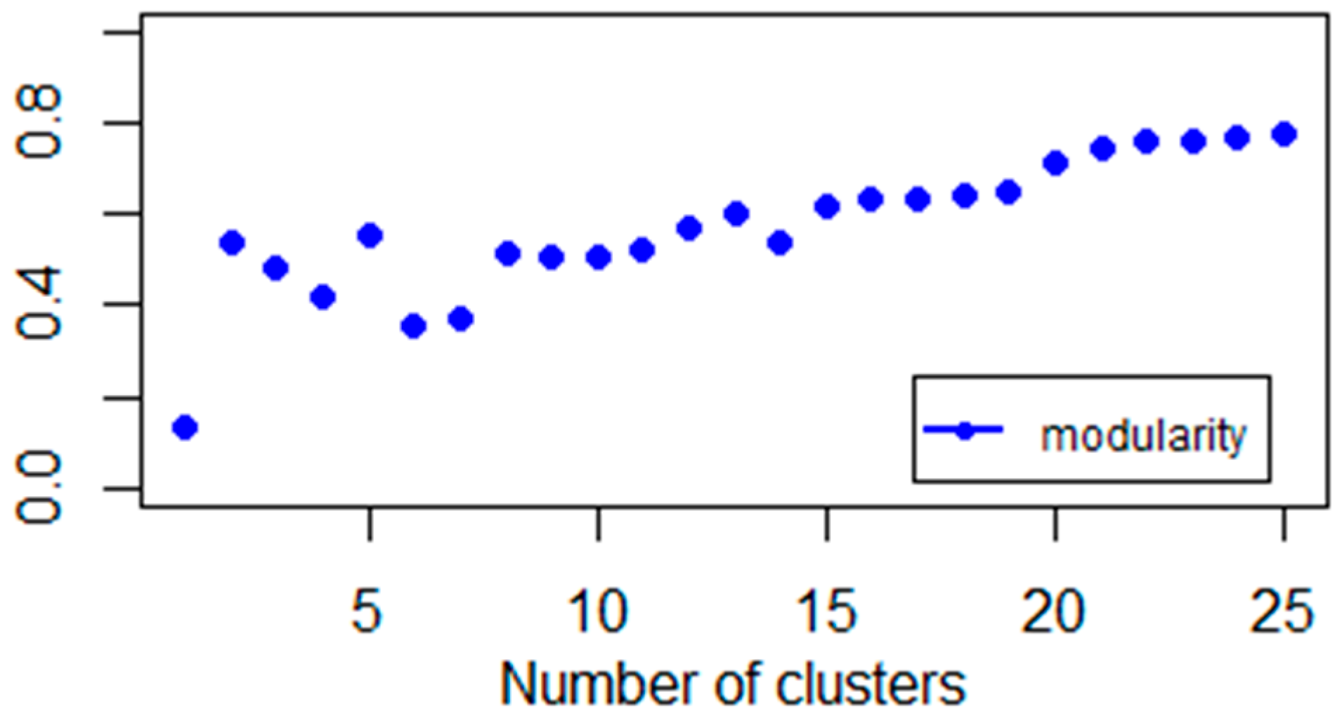
In order to identify the spectrum gap, we apply the elbow method to identify the optimal number of clusters. This approach is rather computationally intensive, because of the percentage of variance explained as a function of clusters has to be estimated (Equation (12)); thus, the whole process has to be repeated many times. However, in our case, as we have 59 stock indices, the elbow method can also be used. Figure 5, Figure 6 and Figure 7 provide evidence for using 2, 3, 4, or 5 clusters.
Analyzing the Gaussian similarity kernel shows that if we randomly generate data, then we would get similarities smaller than 0.2, with probability more than 0.99.
This observation (Figure 6) implies that we have to filter out similarities less than 0.2 from the adjacency matrix.
Figure 2, Figure 3 and Figure 4 show the Gaussian-kernel infers the clearest spectrum property. The relative entropy-based kernel also gives usable results, whereas, jump and correlation-based approaches are ineffective.

3.2. Comparing Normalized Modularity and Laplacian

We propose the use of an accuracy ratio-based (Engelmann et al. 2003) measure to compare the efficiency of different clustering techniques. Calculating the area between the variance explanation function of the random and the different spectral clustering methods generates an appropriate statistic.
Considering this metric (Zhao 2012), it can be seen that the Gaussian-kernel over-performs relative to the entropy-based approach; this is because in each case its variance explanation function is steeper.
Henceforth, the Gaussian-kernel based normalized modularity matrix is used.

3.3. Equity Index Network Structure

Spectral gap (Figure 4) and variance analyses (Figure 5 and Figure 7) imply equity indices can be studied by using 2, 3, and 5 clusters. The explanatory power of two clusters is 38%. This means roughly one-third of the total variance comes from the sample heterogeneity. If we increase the number of clusters and investigate the three cluster cases, we get a similar explanatory power. However, a spectral gap appears between the third and fourth eigenvalues (Figure 4), so, theoretically, we propose the three clusters. The next gap is between the fifth and sixth eigenvalues. The explanation power of five clusters is 52%. This means, half of the total variance of data can be explained by five clusters.
This result (Figure 8) also suggests that additional clusters have little explanatory power, which is in line with spectrum properties.
In practice, mean-variance plots can be used to represent risks and rewards. Intuitively, indices with similar risk and return can be believed to be similar. This approach applies a k-means algorithm to cluster the two-dimensional (mean, standard deviation) representation of logarithmic returns.
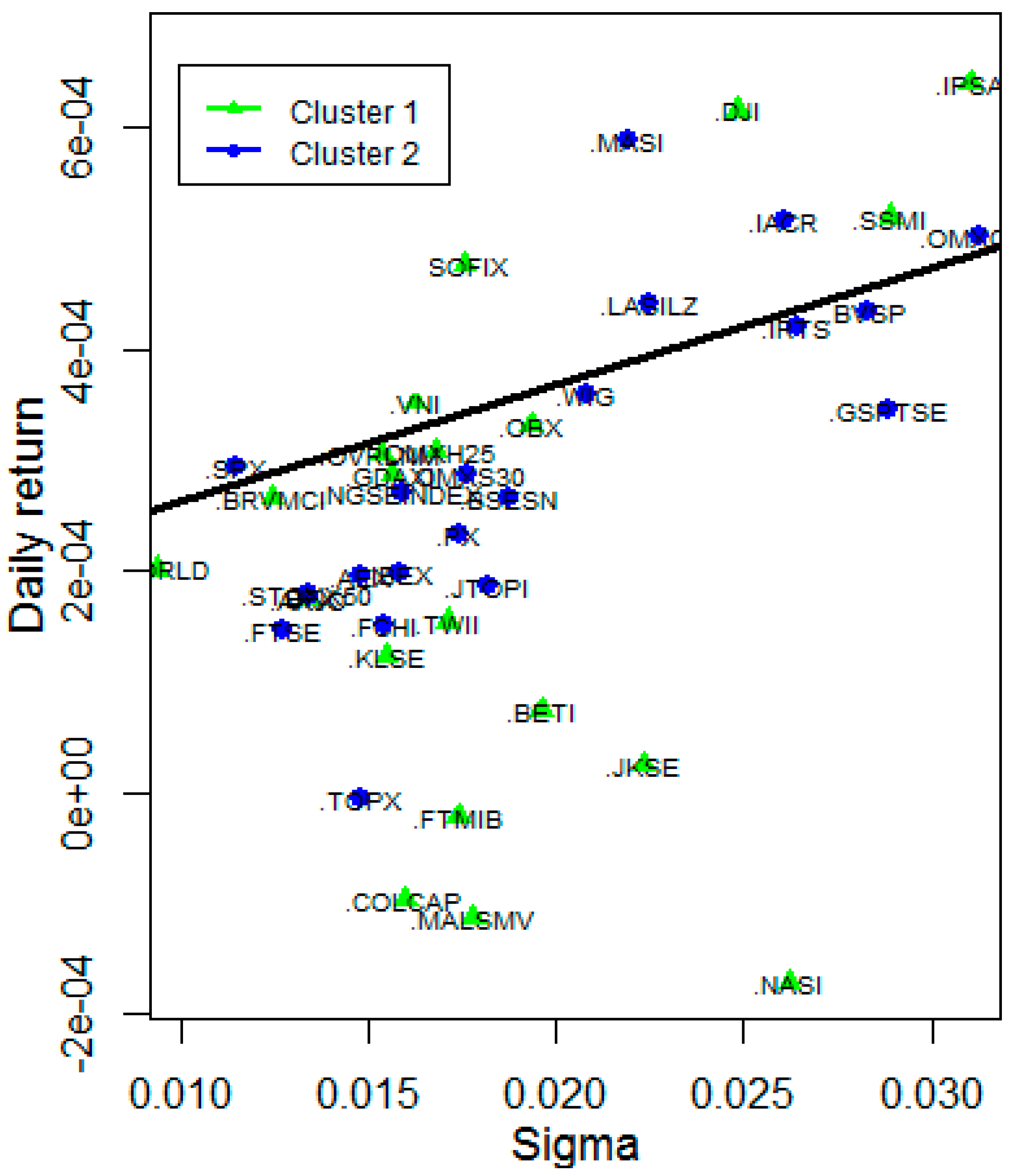
We have seen this naïve method does not give optimal cuts. However, if we calculate Gaussian similarities and normalized modularity matrix based representation, then we get clusters with a higher variance explanatory power. We have seen stock indices can be put into 2, 3, or 5 clusters. If we plot the mean-variance representation of indices we get Figure 9, Figure 10 and Figure 11, for 2 and 5 clusters, respectively.
In Figure 9 we can see clusters that are optimizing the modularity cut are concave in a mean-variance framework. If we have a closer look at the indices in Appendix A (Table A1) we could say that a qualitative approach also works, because east-west geographical clustering would imply almost similar results.
Putting the indices into three different clusters (Figure 10) gives a complicated structure, but we could still state that the first cluster is dominated by European countries, the second by American, and the third is a mixture of indices from the rest of the world. Thus, applying geographical diversification is in line with cluster property. The network generated by simple index returns incorporates geographical information.
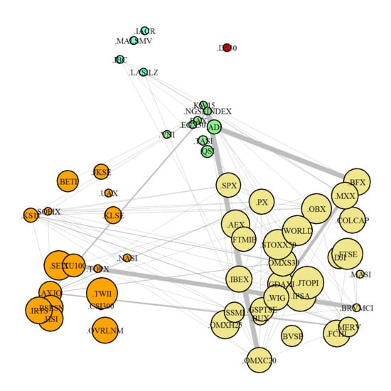
Calculating five different clusters helps us to gain a deeper understanding of the network. The first surprising result is that despite the penalty of different cluster sizes, the Dhaka Stock Exchange (.DS30) is separated into cluster three. In addition, cluster four contains only two African and two American indices. Another interesting result is the first cluster, which includes the Arabian indices except Morocco. Cluster two primarily comprises developed, while cluster five is dominated by emerging market names. Hence, we could notice that spectral clustering-based classification is similar to qualitative categorizations. However, these results also suggest that a portfolios constructed using only geographical scope can integrate indices which behaves significantly differently compared to real regional regimes.
In order to compare our quantitative approach with geographical and MSCI classifications, we run the following regressions:
r = β 0 + β 1 σ + β 2 c l u s t e r +   ϵ ,
The regressions (Table 2) show that spectral clustering provides statistically reliable figures, while geographical- and MSCI-based clusters are not statistically significant.
The outcomes highlight the difficulty of diversification, because the correlation structure of the network is quite homogeneous. Moreover, geographical and other qualitative diversification techniques do not give us statistically significant results. However, indices can be clustered by spectral methods. This means indices in the same cluster are affected by the same risk factor, hence, only cluster wise diversification can be used to eliminate non-systematic global risk.

3.4. Equity Index Graph

Clustering helps us to globally analyze the network. However, the local structure can be better understood by node-specific attributes. Our aim is to find the most influential markets. Hubs can be identified as vertices with the largest vertex weights. Vertex weight of node i can be defined as the sum of the edge weights.
V i : = j = 1 N W i , j δ ( W i j > 0.2 ) ,
Calculating the histograms, we get Figure 12.
The outcomes show that essentially cluster wise histograms differ. In each cluster, there are vertices whose connection numbers substantially differ from the cluster wise mean (Figure 12). Note that the vertex connection density of an Erdő-Rényi graph is binomial, hence hubs and separated nodes cannot be generated (Erdős and Rényi 1960). This implies that preferential attachment processes should be used to model the network structure (Barabási and Albert 1999).
However, the randomness of vertex weights is twofold: one factor is the number of connections, while the other factor is edge weights.
In order to distinguish the effects, we calculate the vertex weights as the sum of connections;
V i c o u n t : = j = 1 N δ ( W i j > 0.2 ) ,
Calculating the histogram of counting-weights we get Figure 13.
We could say clusters 1 and 2 contain hubs, whereas, the vertex-count distribution in cluster 5 is more balanced. There is no hub, but there are vertices with more than 40, and less than 10 connections. The results show that the shape of the cluster wise vertex connection differs, hence, the vertex weight distribution is also a mixed distribution.
Comparing Figure 12 and Figure 13 shows that counting implies higher skewness, while having less effect on the shape. When analyzing edge weights, it turns out that they are not uniformly distributed. In addition, different clusters have different edge weight densities.
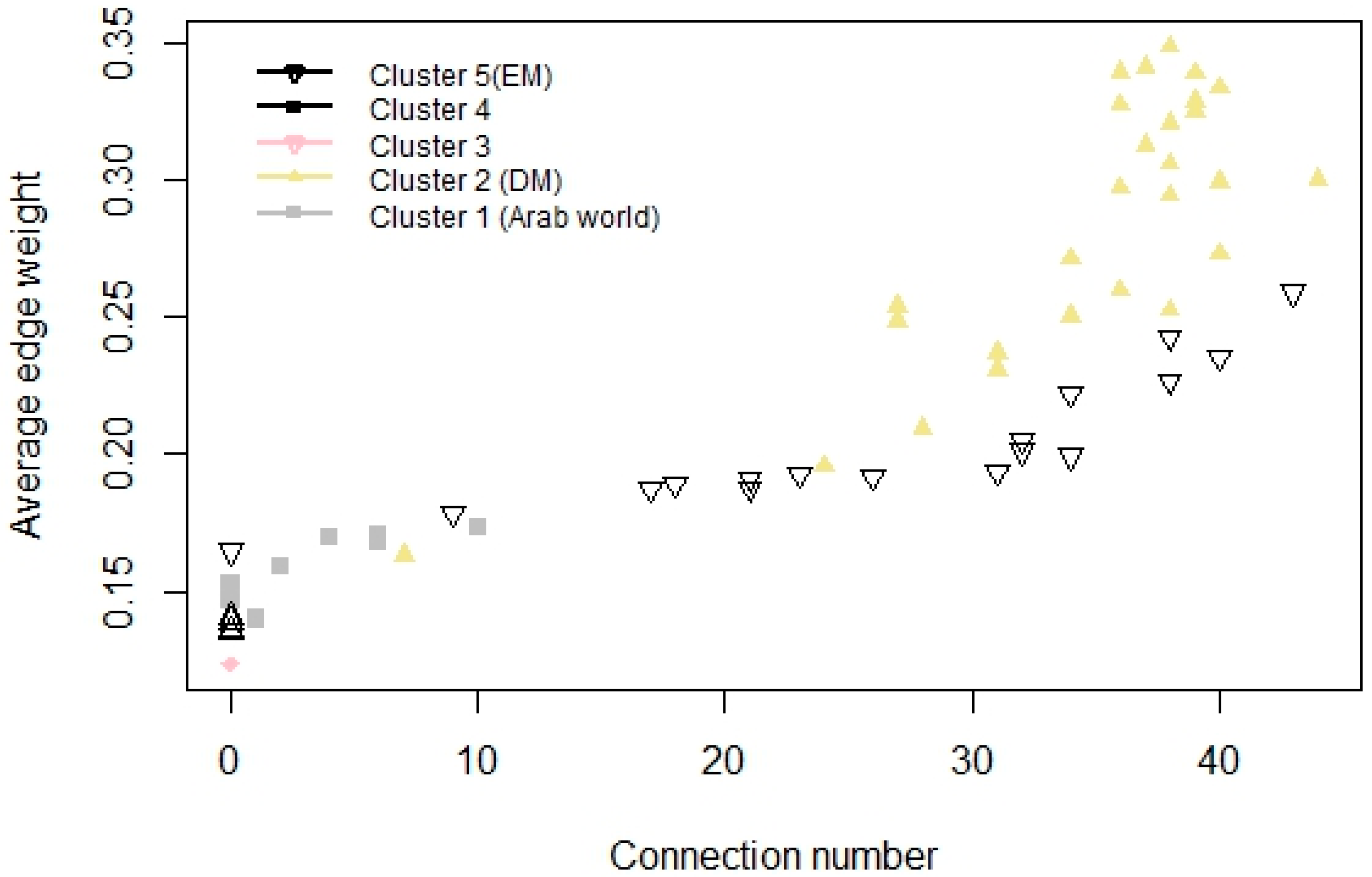
Moreover, it also can be seen (Figure 14), that if the average connection strength is higher, the vertex has more connections; this is true cluster-wise as well.
All of this implies that spectral clustering techniques can be used to distinguish subgraphs. Moreover, the number of connections of an index and its average edge weight, follow the preferential attachment process.

3.5. Risk and Reward

To understand the connection between risk and reward, we can use the mean-standard deviation framework. When calculating the regressions we arrive at Table 3. The outcomes imply that the total sample regression does not provide reliable figures, nevertheless, cluster-wise regressions are significant. This points to the conclusion that the relationship between risk and return, cluster wise has different behavior.
Figure 11 and Table 3 show higher standard deviations, implying higher returns, because regression lines slope upwards. In addition, it also turns out that connections between returns and standard deviations are strong in Arabian and developed market cases. Nevertheless, emerging markets show different statistics: index returns in the fifth cluster are not linear in standard deviation, hence emerging market returns cannot be estimated in the Markowitz framework.

3.6 Time Stability

Making investment decisions vastly depends on the time stability of our strategy. Therefore, we have to check the stationarity of our clustering method. By splitting the time series by years we get 25 periods. Calculating the stability of explained percentage variance of clustering could be a good proxy of time stability. Stationarity can be analyzed by the augmented Dicky–Fuller (ADF) test.
Note that, the analysis covers 25 years’ data, hence we get 25 non-overlapping periods. The t-values (Table 4) show that the variance explanation power process could be stationer, but because of the small sample size the ADF p-value of 0.32. To gain a better understanding of the results, we can compare them with the test statistics of randomly generated 25 long standard normal samples (Figure 15).
However, we also have to study the time stability of cluster wise mean-standard deviation regressions. Splitting the data into one-year periods, clustering them and calculating regressions shed some light on the robustness of clusters (Figure 16).
The results show that cluster wise mean-variance regressions are stationary in cluster 1 and 2. Nevertheless, cluster 3 and 4 are outliers and clusters 5 mostly covers emerging market names. Thus, the Gaussian-based normalized modularity clustering technique can be used to filter out outliers and find robust clusters.

4. Discussion

Spectral clustering techniques can be used to discover the equity index structure. On the one hand, clusters help us to overcome the hardship of heterogeneity and make diversification more efficient. In our paper we shed some light on the relations between spectral, geographical and qualitative clustering. It also turned out that Gaussian-kernel based clusters are more suitable than geographical and qualitative categorizations. In addition, spectral cluster-wise linear regressions give time stationary and significant results.
On the other hand, we stress that correlation does not convey enough information about the network; hence linear dependency-based diversification is not optimal (Sharpe 1964; Maldonado and Anthony 1981). We compared various similarity kernels and spectral clustering methods to demonstrate the inadequacy of a normalized Laplacian approach (Takumasa 2015) and underpin the applicability of the proposed Newman–Girvan cut. Moreover, we highlighted that daily closing prices incorporate the network level information. The results unveiled that tail events have little effect on the dense network structure, in other words, market shocks have no effect on the cluster components; thus, index co-movements are not affected by large price changes.
All of these imply spectral clustering can eliminate non-linear effects, thus regular mean-standard deviation representation gives cluster-wise reliable figures. Instead of qualitative categorization, we suggest that portfolio managers should use Gaussian-based normalized modularity clusters to diversify global non-systematic risk.
An interesting field of further research would be analyzing the evolution of the network to identify patterns that could help us to understand the life cycle of hubs and the vulnerability of the current equity network.

Author Contributions

Conceptualization, L.N. and M.O.; Methodology, L.N. and M.O.; Validation, L.N. and M.O.; Formal Analysis, L.N. and M.O.; Investigation, L.N. and M.O.; Writing-Original Draft Preparation, L.N. and M.O.; Writing-Review & Editing, L.N. and M.O.; Visualization, L.N.; Supervision, M.O.

Funding

Research fund was provided by Pallas Athéné Domus Educationis.

Acknowledgments

The authors would like to gratefully acknowledge the valuable comments and suggestions of three anonymous referees that contributed to a substantially improved paper. Mihály Ormos acknowledges the support of the János Bolyai Research Scholarship of the Hungarian Academy of Sciences and the support of the Pallas Athéné Domus Educationis Foundation. The views expressed are those of the authors and do not necessarily reflect the official opinion of the Pallas Athéné Domus Educationis Foundation.

Conflicts of Interest

The authors declare no conflict of interest. The funders had no role in the design of the study; in the collection, analyses, or interpretation of data; in the writing of the manuscript; or in the decision to publish the results.

Appendix A

Table A1. Clusters of stock indices.
CountryTwo ClustersThree ClustersFive Clusters
United Arab Emirates231
Saudi Arabia231
Qatar211
Kuwait211
Egypt231
Bahrain211
Vietnam211
Nigeria211
Dow Jones122
Denmark112
Switzerland112
Canada122
Mexico122
Chile122
Argentina122
Hungary112
Morocco212
S&P 500122
MSCI World122
Czech Republic112
Togo212
Spain112
Norway112
Luxembourg112
France112
South Africa132
Euro Stocks112
Sweden112
UK112
Netherlands112
Finland112
Poland132
Germany112
Belgium112
Italy112
Brazil122
Colombia132
Bangladesh213
Costa Rica214
Zambia214
Malawi214
Venezuela214
South Korea235
Hong Kong235
Thailand235
China235
Kenya235
India235
Namibia235
Turkey235
Indonesia235
Malaysia235
Russia235
Australia235
Taiwan235
Japan235
Ukraine235
Bulgaria215
Romania235
Notes: This table contains the list of indices and clustering results for 2, 3, and 5 clusters.

References

  1. Barabási, Albert L., and Albert Réka. 1999. Emergence of Scaling in Random Networks. Science 26: 509–12. [Google Scholar] [CrossRef]
  2. Berlinet, Alain, and Thomas-Agnan Christine. 2011. Reproducing Kernel Hilbert Spaces in Probability and Statistics. Berlin: Springer Science & Business Media, pp. 1–108. ISBN 978-1441990969. [Google Scholar]
  3. Bolla, Marianna. 2011. Penalized version of Newman-Girvan modularity and their relation to normalized cuts and k-means clustering. Physical Review E 84: 016108. [Google Scholar] [CrossRef] [PubMed]
  4. Chung, Fan R. G. 1997. Spectral Graph Theory. Providence: American Mathematical Society, No. 92. pp. 14–81. ISBN 978-0821803158. [Google Scholar]
  5. Engelmann, Bernd, Evelyn Hayden, and Dirk Tasche. 2003. Measuring the Discriminative Power of Rating Systems. Banking and Financial Supervision. Frankfurt: Deutsche Bundesbank. [Google Scholar]
  6. Erdős, Péter, and Rényi Alfréd. 1960. On the Evolution of Random Graphs. Acta Mathematica Hungarica 5: 17–61. [Google Scholar]
  7. Erdős, Péter, Mihály Ormos, and Dávid Zibriczky. 2011. Non-parametric and semi-parametric asset pricing. Economic Modelling 28: 1150–62. [Google Scholar] [CrossRef]
  8. Fama, Eugene, and Kenneth R. French. 1996. Multifactor explanations of asset pricing anomalies. The Journal of Finance 51: 55–84. [Google Scholar] [CrossRef]
  9. Maurizio, Filippone, Francesco Camastra, Francesco Masulli, and Stefano Rovetta. 2007. A survey of kernel and spectral methods for clustering. Pattern Recognition 41: 176–90. [Google Scholar] [CrossRef]
  10. Heiberger, Raphael H. 2014. Stock network stability in times of crisis. Physica A: Statistical Mechanics and Its Applications 393: 376–81. [Google Scholar] [CrossRef]
  11. Gregory, Leibon, Scott Pauls, Daniel Rockmore, and Robert Savell. 2008. Topological Structures in the Equities Market Network. PNAS 105: 20589–94. [Google Scholar] [CrossRef]
  12. Von Luxburg, Ulrike. 2007. Tutorial on Spectral Clustering. Statistics and Computing 17: 395–416. [Google Scholar] [CrossRef]
  13. Maldonado, Rita, and Saunders Anthony. 1981. International portfolio diversification and the inter-temporal stability of international stock market relationships, 1957–1978. Financial Management 10: 54–63. [Google Scholar] [CrossRef]
  14. MSCI. 2018. Market Classification. Available online: https://www.msci.com/market-classification (accessed on 3 November 2018).
  15. Ormos, Mihály, and Dávid Zibriczky. 2014. Entropy-Based Financial Asset Pricing. PLoS ONE 9: E115742. [Google Scholar] [CrossRef] [PubMed]
  16. Shi, Jianbo, and Jitendra Malik. 2000. Normalized cuts and image segmentation. IEEE Pattern Analysis and Machine Intelligence 22: 888–905. [Google Scholar] [CrossRef] [Green Version]
  17. Sharpe, William F. 1964. Capital asset prices: A theory of market equilibrium under conditions of risk. Journal of Finance 19: 425–42. [Google Scholar]
  18. Song, Dong-Ming, Michele Tumminello, Wei-Xing Zhou, and Rosario N. Mantegna. 2011. Evolution of worldwide stock markets, correlation structure, and correlation-based graphs. Physical Review E 84: 026108. [Google Scholar] [CrossRef] [PubMed]
  19. Takumasa, Sakakibara, Tohgoroh Matsuib, Atsuko Mutoha, and Nobuhiro Inuzuka. 2015. Clustering mutual funds based on investment similarity. Procedia Computer Science 60: 881–90. [Google Scholar] [CrossRef]
  20. Yalamova, Rossitsa. 2009. Correlations in Financial Time Series during Extreme Events-Spectral Clustering and Partition Decoupling Method. Paper presented at World Congress on Engineering, London, UK, July 1–3; Volume 2, pp. 1376–78. [Google Scholar]
  21. Zhao, Yanchang. 2012. R and Data Mining: Examples and Case Study. Cambridge: Academic Press, pp. 49–59. [Google Scholar]
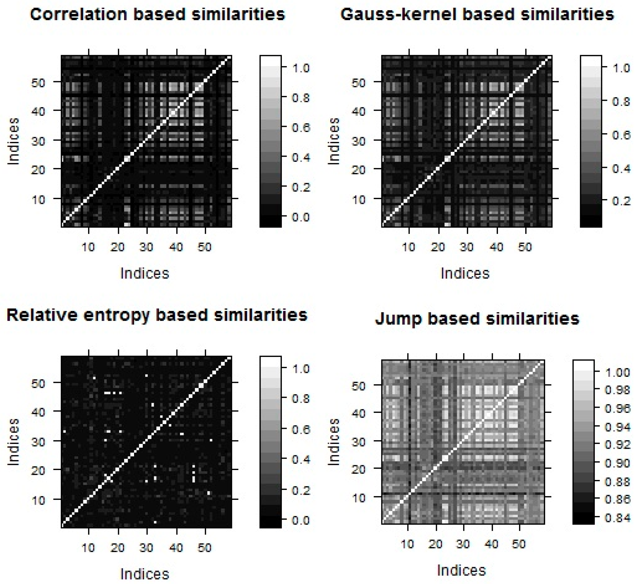
Figure 1. Level plots of daily similarity matrices.
Jrfm 11 00088 g001
Figure 2. Eigenvalues of normalized modularity matrix in decreasing order.
Jrfm 11 00088 g002
Figure 3. Eigenvalues of normalized Laplacian matrix in decreasing order.
Jrfm 11 00088 g003
Figure 4. Largest eigenvalues of Gaussian- and relative entropy-based normalized modularity matrices.
Jrfm 11 00088 g004
Figure 5. Explained percentage variance of Gaussian-kernel based clusters of representations.
Jrfm 11 00088 g005
Figure 6. Histogram of 10,000 Gaussian similarities which are generated from i.i.d. 250 dim. standard normal samples.
Jrfm 11 00088 g006
Figure 7. Explained percentage variance of Gaussian-kernel based clusters after zero out similarities less than 0.2.
Jrfm 11 00088 g007
Figure 8. Explained percentage variance of Gaussian-kernel based clusters.
Jrfm 11 00088 g008
Figure 9. Two Gaussian-kernel based normalized modularity clusters (part of the total graph).
Jrfm 11 00088 g009
Figure 10. Three Gaussian-kernel based normalized modularity clusters, edges with weights stronger than 0.5.
Jrfm 11 00088 g010
Figure 11. Five Gaussian-kernel based normalized modularity clusters.
Jrfm 11 00088 g011
Figure 12. Histogram of vertex weights, five Gaussian cluster, two nodes are connected if their Gaussian similarity is stronger than 0.2.
Jrfm 11 00088 g012
Figure 13. Histogram of vertex count-weights, five Gaussian cluster, two nodes are connected if their similarity is stronger than 0.2.
Jrfm 11 00088 g013
Figure 14. Cluster-wise connection number and average connection strength.
Jrfm 11 00088 g014
Figure 15. Histogram of ADF statistics of 10,000 independent 25 dim. standard normal sample.
Jrfm 11 00088 g015
Figure 16. ADF test of cluster wise time shifted regressions.
Jrfm 11 00088 g016
Table 1. Descriptive statistics of monthly returns.
IndexMeanVarianceSkewness
.CSI3000.0180.056−0.336
.XU10000.026−0.809
.DJI0.0120.009−0.819
.UAX−0.0340.037−0.721
.WORLD0.0040.002−1.889
Notes: Table 1 shows the descriptive statistics of the monthly returns, where CSI300, XU100, DJI, UAX, and WORLD represent the Shanghai Composite 300, Brose Istanbul 100, Dow Jones, Ukraine UX index, and the MSCI World index respectively.
Table 2. Regression statistics.
MethodCoeff. of Clusterp-Value
Geographical−0.0000360.394
MSCI−0.0000410.293
Spectral−0.0001120.027
Notes: This table shows the daily linear regression coefficients and p statistics of geographical, MSCI, and spectral clusters. Returns are regressed on standard deviations and clusters.
Table 3. Descriptive statistics of daily linear regressions.
Clustersp-Value of Interceptp-Value of s.d. R 2
Total Sample0.620.120.05
First cluster0.620.020.68
Second cluster0.290.000.59
Fifth cluster0.930.710.01
Notes: This table shows the p statistics and R 2 values of daily linear regressions. Returns are regressed on standard deviations. Calculation is done for total, only the first, second and fifth clusters.
Table 4. Augmented Dicky–Fuller (ADF) statistic of explained percentage variance process.
ADF t-ValueADF p-Value
−2.670.32
Notes: This table shows the ADF t and p statistics of yearly percentage variance process.