Abstract
This paper offers an empirical characterization of the relation between the international price of oil and exchange rates that is both useful and reliable. Our characterization is useful because it rests on information of asset prices that are determined in functioning asset markets. Our characterization is reliable because its maintained assumptions are not rejected by the data. Four features differentiate our work from previous analyses. First, our reliance on bilateral rates opens previously ignored financial arbitrage opportunities between oil prices and exchange rates. Second, our emphasis on statistical testing makes our characterization empirically reliable. Specifically, we use a vector-error correction modeling strategy in which both oil prices and exchange rates are endogenous. This framework allows testing for the existence of an arbitrage relation, for the direction of causality, for parameter constancy, for white noise residuals, and for forecast accuracy. Third our reliance on data through 2020 makes our analysis timely. Fourth, to emphasize the advantages of our approach, we compare our results to those derived for formulations relying on effective exchange-rate indexes.
1. Introduction
This paper offers an empirical characterization of the relation between movements in the price of oil and movements in bilateral exchange rates. Four features differentiate our work from previous analyses. First, our reliance on bilateral rates opens up previously ignored financial arbitrage opportunities between oil prices and exchange rates.1 Second, our emphasis on statistical testing makes our characterization empirically reliable. To this end, we use a vector-error correction modeling strategy in which both oil prices and exchange rates are endogenous. This framework allows testing for the existence of an arbitrage relation, for the direction of causality, for parameter constancy, for white noise residuals, and for forecast accuracy. Third our reliance on data through 2020 makes our analysis timely. Specifically, we compare models’ forecasts from January 2019 to April 2020, when the price of oil was negative for the first time.2 Fourth, to emphasize the advantages of our approach, we compare our results to those derived for formulations relying on effective exchange-rate indexes.
Section 2 shows the relevant empirical studies of the relation between the price of oil and exchange rates.3 Half of the studies rely on samples that exclude developments since 2008 and two thirds of all studies rely on effective exchange-rate indexes. Section 3 describes the pitfalls of using real effective exchange-rate indexes. For this paper, the main pitfall is that for the effective exchange-rate index to be helpful, all the bilateral rates need to change in the same direction and proportion, which is not observed in foreign exchange markets. Section 4 develops our empirical application using the currencies included in the IMF’s Special Drawing Right (SDR): The U.S. dollar, the euro, the yen, the pound sterling, and the renminbi.4 For estimation, we use monthly observations from January 1999 (the introduction of the Euro) to April 2020 (the collapse of oil prices).5 The results show a statistically reliable arbitrage relation between oil prices and bilateral exchange rates.
2. Previous Work
The theoretical work in this area began with Krugman (1980) and Golub (1983). They focused on how bilateral exchange rates responded to exogenous changes in the price of oil. The subsequent empirical literature (Table 1A) has retained the two-country framework by using effective exchange-rate indexes.6 Finally, even though China is the largest economy in the world7 and the renminbi is now included in the SDR, the role of China has been largely neglected in this literature.8

Table 1.
(A) Design Characteristics of Selected Studies (by publication date). (B) Reported Statistical Tests of Selected Studies (by publication date).
For estimation, the literature reports little or no evidence on the reliability of their findings (Table 1B).9 Key questions regarding parameter constancy, residuals’ properties, forecast accuracy, and stationarity are generally not reported. Why, then, should we rely on their conclusions if we cannot assess their statistical reliability?
3. Real Effective Exchange Rates
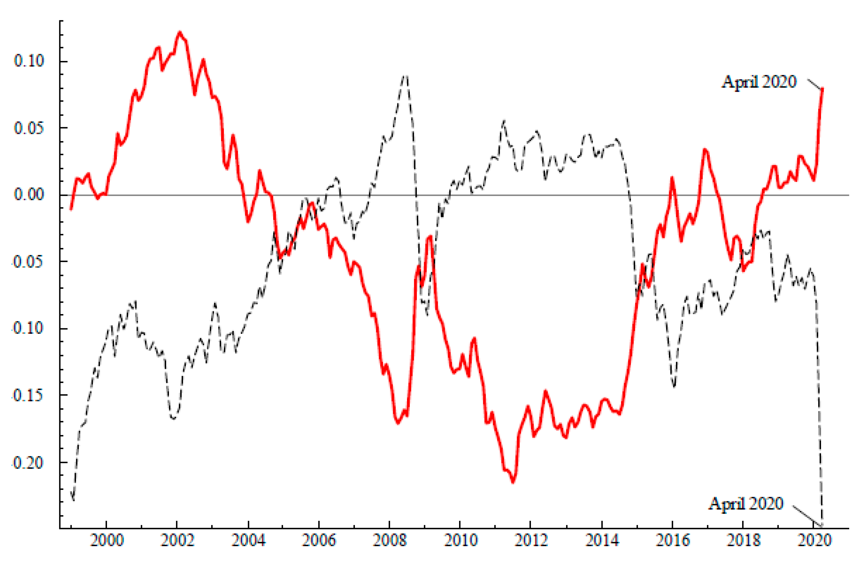
Figure 1 shows the relation between the real price of oil and the Fed’s real effective exchange-rate index. That there is a strong relation is clear: Since 1999, real appreciations of the dollar are associated with declines in the real price of oil, even during the unprecedented changes of the first quarter of 2020. What is not clear is how this information helps the management of financial risks, given that there is no financial market in which the Fed’s measure of the dollar is internationally traded. To see how aggregation can create such a correlation we now focus on the measurement of the Fed’s index.

Figure 1.
The dashed line is the West Texas Intermediate (WTI) price of oil delineated by the U.S. CPI; the solid line is the Federal Reserve’s broad measure for real effective exchange rate (FX/$). Variables are expressed in logarithms. The mean and range of the series are matched.
3.1. Measurement
The Federal Reserve Board’s measure of the real effective exchange rate uses chained aggregation of 26 bilateral exchange rates. These exchange rates are adjusted for differentials in CPI movements relative to U.S. CPI; the selected currencies are associated with the bulk of U.S. trade. The formula is
where is the nominal price of the U.S. dollar in terms of the ith currency, is the consumer price index for the jth country, and is the “total” trade share (Leahy 1998).10 is the share of U.S. non-oil imports from the ith country, is the share of U.S. of non-oil exports to the ith country, is the share of imports of the ith country coming from the kth country, and is the share of imports of the ith country coming from the jth country (Leahy 1998).11 To measure the level of D, one selects a base period in which = 100 with the level of the index for all other periods defined recursively. Note, however, that for the purposes of this paper, aggregation of bilateral exchange rates implies the existence of an active market for D.
3.2. Limitations
By construction, movements in owe to changes in both exchange rates and weights:
Thus, the first limitation is that movements in the effective exchange rates cannot be uniquely mapped into movements in bilateral rates. This consideration undermines the usefulness of Figure 1 for hedging strategies and managing financial risks.
Second, movements in the effective value of the dollar owe to changes in both exchange rates and weights, and thus one cannot identify whether the relation in Figure 1 is between oil prices and trade weights or between oil prices and exchange rates. Specifically, if all the bilateral real exchange rates were unchanged, then
Thus, one cannot identify whether the relation of Figure 1 is between oil prices and trade weights or between oil prices and exchange rates.12 In brief, for practitioners interested in the question of “how do we know?” the identification problems associated with effective exchange-rate indexes cannot be avoided: How do we know that the relation is between the price of oil and exchange rates and not between the price of oil and weights of the aggregate? How do we know that a particular currency is responsible for a movement in D and not a combination of other currencies?
Third, and just as an illustration, suppose that where P is the real price of oil. Then the ceteris paribus effect of a change in the ith currency on lnP is which depends on how much the country (or countries) with the ith currency trade with the United States. If that trade is zero, then that currency is irrelevant for oil prices regardless of the importance of that country for the international oil market.13 Avoiding this limitation involves assuming that all currencies change by the same proportion, which contradicts the data on exchange rates (Figure 2).
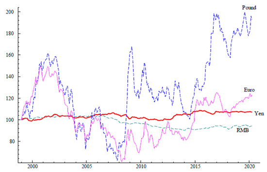
Figure 2.
Bilateral Real Exchange Rates for the Currencies in the Special Drawing Right (SDR). Series are set 1999 = 100.
Fourth, the weights are not independent of oil prices, especially the weights for the third country effects 14 Data for these shares come from the IMF’s Direction of Trade and include the value of trade in oil. To the extent that movements in the value of oil trade are dominated in the short run by movements in oil prices, then reliance on effective exchange rates uses the price of oil to explain the price of oil. Finally, the weights for non-oil bilateral trade are not measured on a value added basis. To the extent that non-oil imports include goods that were produced with oil, then the weights are contaminated by oil prices.15
4. Analysis
4.1. Unconditional Correlations
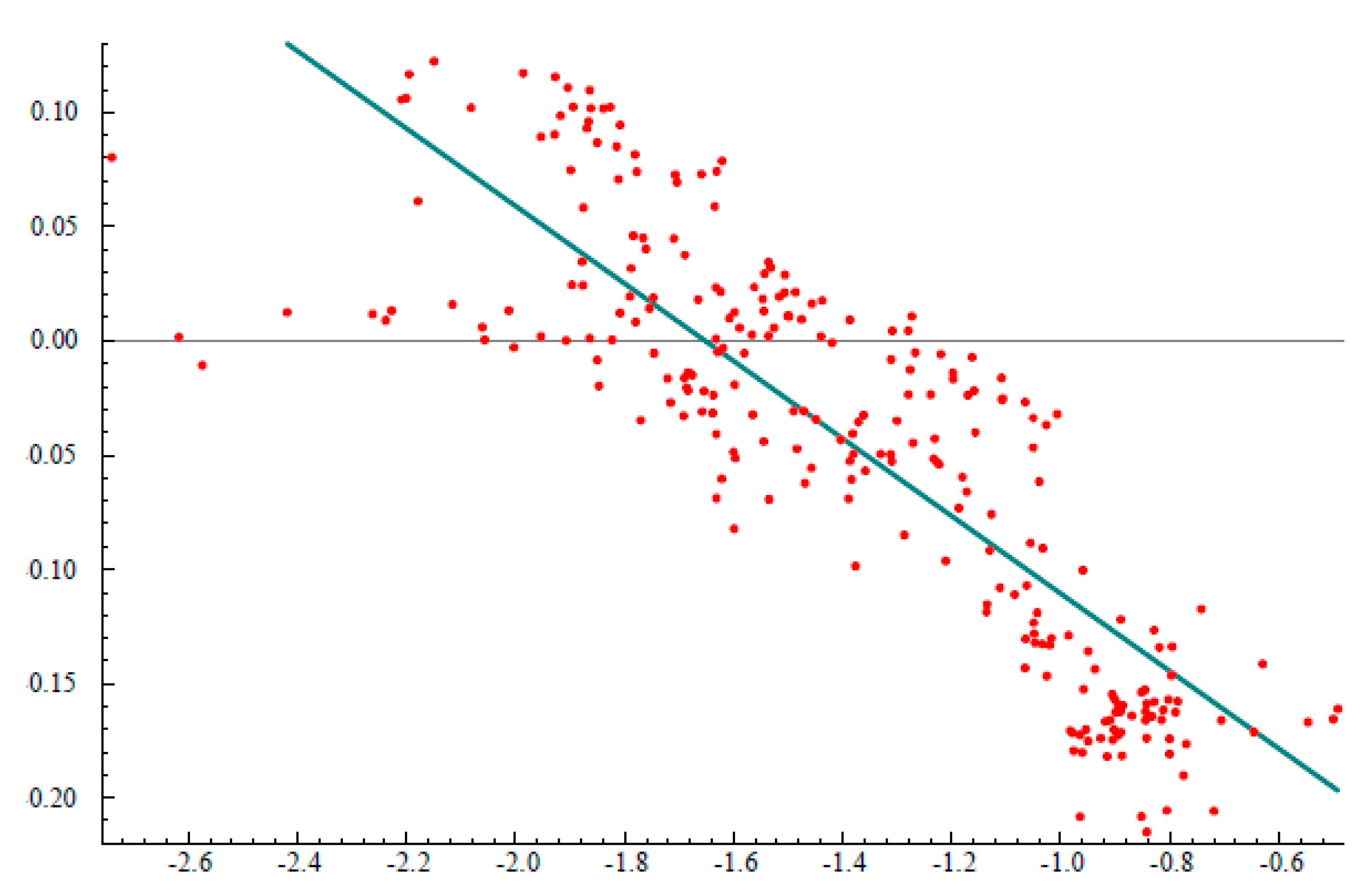
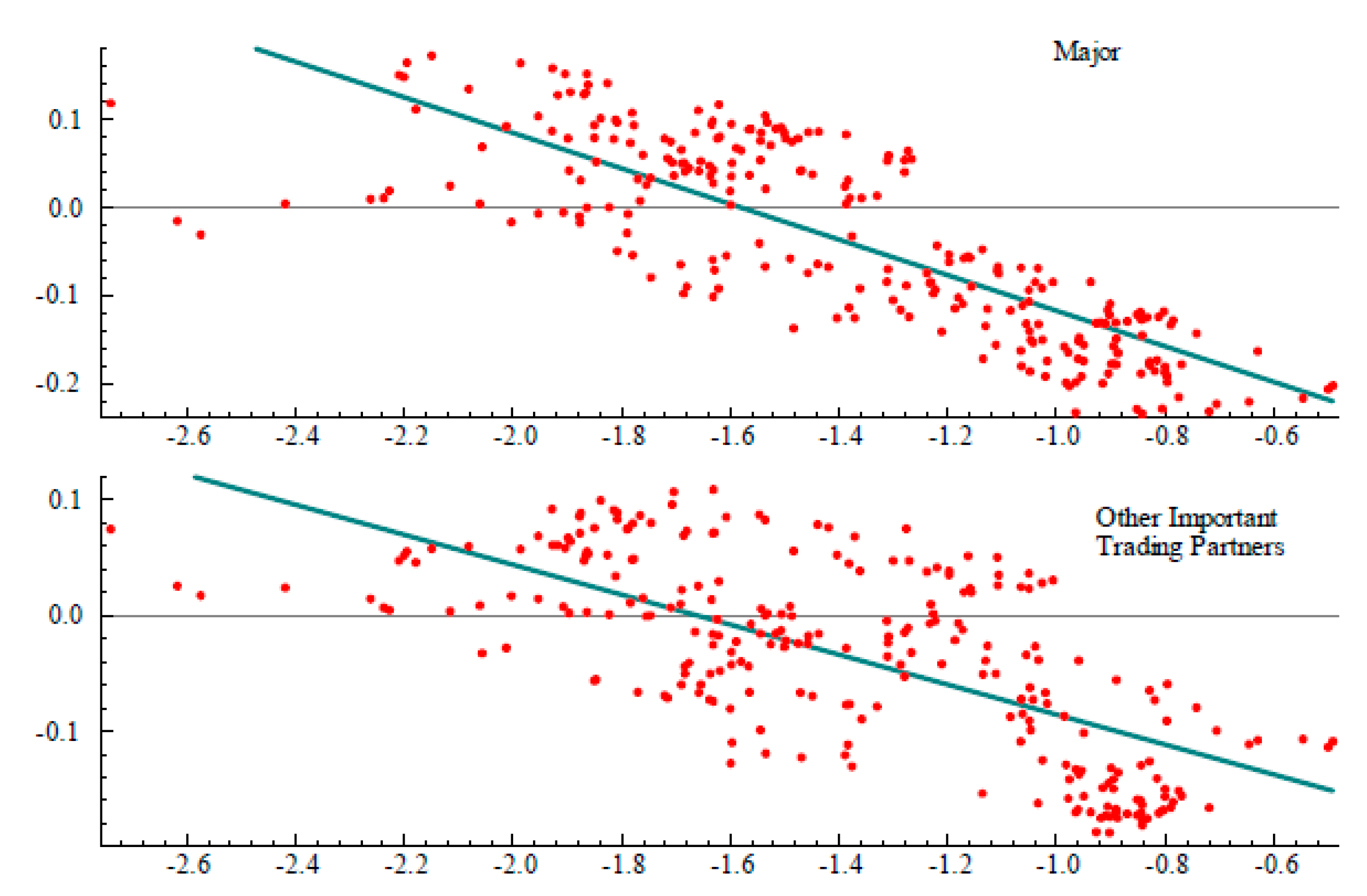
Figure 3 shows the scatter plot between the broad real effective exchange-rate index and the real price of oil. There is no question about the strength of this correlation. To examine whether this correlation is sensitive to the currency mix, Figure 4 shows the scatter plot using the Federal Reserve’s effective exchange-rate indexes for Major Currencies and for Other Important Trading Partners. Again, the evidence shows a strong and inverse association between the real price of oil and these two real effective exchange-rate indexes.
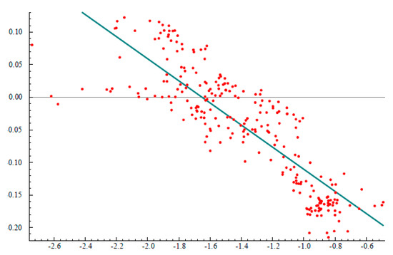
Figure 3.
The horizontal axis represents the WTI price of oil deflated by the U.S. CPI; the vertical axis represents the Federal Reserve’s broad measure for the real effective exchange rate. Variables are expressed in logarithms.
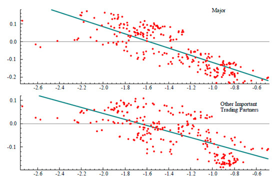
Figure 4.
The horizontal axis represents the WTI price of oil deflated by the U.S. CPI; the vertical axis for the top panel represents the Federal Reserve’s measure for the real effective exchange rate for the major currencies. The vertical axis for the bottom panel represents the Federal Reserve’s measure for real effective exchange rate for the Other Important Trading Partners’ currencies. Variables are expressed in logarithms.
But if we consider the relation between the real price of oil and each of the bilateral currencies (Figure 5), then we find that the unconditional correlations are sensitive to the currency. Indeed, the relation for the yen is absent and the one for the renminbi is driven by outliers. This result emphasizes that reliance on the effective exchange-rate index embodies a fallacy of composition: that what holds for D holds exactly for each of its components.
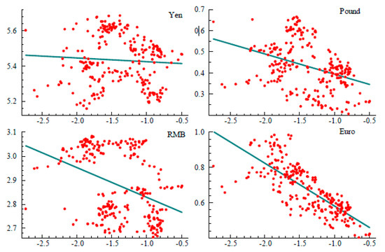
Figure 5.
The horizontal axis represents the WTI price of oil deflated by the U.S. CPI; the vertical axis for each panel represents the bilateral exchange rate adjusted by movements in that currency’s CPI relative to the U.S. CPI. Variables are in logarithms.
4.2. Vector Error Correction Framework
We use a vector error correction model treating both oil prices and exchange rates as en- dogenous. Specifically,
where and is a polynomial of order 6 in the lag operator L and is a matrix of unknown coefficients; the specification includes seasonal dummies. This approach has two advantages: it addresses the spurious regression critique and differentiates between short- and long-run responses to shocks. In addition, Equation (1) allows us to conduct out-of-sample forecasts, to evaluate the properties of the residuals, and to test the assumed constancy of the parameters.
Empirically, the existence of an arbitrage relation depends on the rank of . If the rank equals one, then
and y = 0 represents the arbitrage condition, with being the associated coefficients; characterizes responsiveness of y to deviations from the arbitrage condition. We assess the sensitivity of the results using three alternative measures of the dollar:
- Model 1:
- Effective Broad yt = (pt dt)’
- Model 2:
- Effective, Major and Other Trading Partners yt = (pt dmt dot)’
- Model 3:
- Bilateral rates yt
where variables in lower case denote logarithms and
- p is the real price of oil
- d is the broad measure of the dollar
- dt is the measure of the dollar for the major currencies
- do is the measure for other important trading partners
- is the price-adjusted price of the dollar in terms of the yen
- is the price-adjusted price of the dollar in terms of the euro
- is the price-adjusted price of the dollar in terms of the pound
- is the price-adjusted price of the dollar in terms of the renminbi.
For model 3, the no-arbitrage condition y = 0 can be re-written as
Importantly, this equation is not determining p in terms of or the other way around. Rather, this equation is the long-run, no-arbitrage equilibrium relation between p and the . Thus, shocks that create arbitrage opportunities which then trigger changes in all of the endogenous variables as indicated in Equation (1). We now proceed to examine whether the rank of is one.
4.2.1. Time-Series Properties
Stationarity: A necessary condition for cointegration is Π·y = 0 which implies that y is non-stationary. To test stationarity, we use monthly observations from January 1999 to April 2020 and rely on Augmented Dickey Fuller tests. Appendix A.2 shows that one cannot reject the hypothesis that log-levels of the variables are integrated of order one.
Granger Causality: A property of interest is whether exchange rates Granger-cause the price of oil or the other way around. For example, model 3 has five equations and each variable has six lags. The null hypothesis that exchange rates do not Granger cause the price of oil involves excluding all the exchange rates from the equation for the price of oil; this exclusion involves zeroing 24 coefficients. Similarly, the null hypothesis that the price of oil does not Granger-cause exchange rates involves setting the six coefficients for oil prices to zero in each of the four exchange rate equations for a total of 24 zero restrictions. These two hypotheses are tested with a χ2(n) test where n is the number of restrictions; Table 2 displays the results.

Table 2.
Granger Causality Tests: 1999:1–2020:4.
According to the results, exchange rates Granger-cause the real price of oil for the three models. In other words, excluding exchange rates from the equation for the price of oil carries a statistically significant loss of information. The results also indicate that the price of oil Granger-causes the real bilateral exchange rates but not the real effective exchange rates. In other words, models using bilateral exchange rates embody global interdependencies in which real oil prices and real bilateral rates are jointly determined.
4.2.2. Cointegration
Having established that the series are integrated of order one, we now estimate the rank of using Johansen’s Trace and Max tests, corrected for degrees of freedom (Johansen 1988). This method begins by testing whether the rank of is zero. If this hypothesis is not rejected, then the arbitrage relation between oil prices and exchange rates is absent. If this hypothesis is rejected, then Johansen tests whether the rank of is one. If this hypothesis cannot be rejected, then the rank of is one and there is just one linear combination of the levels of the real price of oil and real exchange rates that is stationary-that is, the no-arbitrage condition.16
For estimation, we use monthly data from January 1999 to December 2018; observations from January 2019 to April 2020 are reserved for out-of-sample forecasting. The estimation results are shown in Table 3.

Table 3.
p-Values for Johansen’s Rank Tests 1999:1–2018:12.
The evidence rejects the null hypothesis that the rank of is zero for all three models. Further, the evidence cannot reject the null hypothesis that the rank of is one for all three models. Taken together, these results suggest the existence of one cointegration relation between the real price of oil and real exchange rates, however measured. The associated cointegration coefficient estimates are shown in Table 4.

Table 4.
Cointegration Results—1999:1–2018:12-Johansen Method.
The adjustment coefficients (the αs) for the oil price is significant and negative in all cases and they vary from −0.12 to −0.14, meaning that the adjustment to the long run is less than one year if all else is constant. The adjustment coefficients associated with exchange rates are negligible and insignificant. This result owes to volatility of exchange rates exceeding the volatility of oil prices.
The cointegration coefficients (the βs) for the effective exchange rates are significant (models 1 and 2): a one percent real appreciation in the dollar is associated with a decline in the real price of oil ranging from a nearly four percent for model 1 to a 2.6 percent decline for model 2 when using dm; note that the coefficient for the measure of Other Trading Partners is barely significant. If taken at face value, this result suggests that the renminbi is not a relevant asset price for arbitrage, even though China has the third largest share of world oil consumption.17
The coefficient estimates for model 3 reveal several features of interest. First, the no-arbitrage equation is
which indicates that real appreciations of these currencies are associated with a decline in the price of oil.18 Second, only the coefficients for the euro and the renminbi are significant; this result is not surprising given the importance of these two economies for both the oil and the foreign-exchange markets. Indeed, the Euro area and China are the largest oil consumers (after the United States) and account for a 29% of world oil consumption in 2019. Third, the significance of the estimate for the renminbi contrasts with the results of model 2, which implies that the renminbi is not relevant for arbitrage. Fourth, there is a significant asymmetry in the coefficients for the euro and the renminbi: the coefficient for is nearly twice the coefficient for . This asymmetry implies that identical percent changes in these two exchange rates have a differential effect on the price of oil because of the greater extent to which the euro is used in financial transactions globally.19 In other words, the differential in the coefficient estimates reflects the greater economic importance of the euro relative to the renminbi.20
Finally, and at the risk of stating the obvious, differences in coefficient estimates across models are not due to differences in sample periods or estimation methods or econometric specifications: these design features are identical for the three models. Instead, the differences in estimates are due to the pitfalls of aggregation.
Residuals Properties: Table 5 reports the test results associated with the maintained assumptions used in estimation: serial independence, normality, and homoskedasticity. The results show that the residuals generally satisfy these assumptions but, to be sure, there are exceptions; this consideration needs to be considered when assessing the usefulness of the results.

Table 5.
p-Values for statistical properties of residuals 1999:1–2018:12.
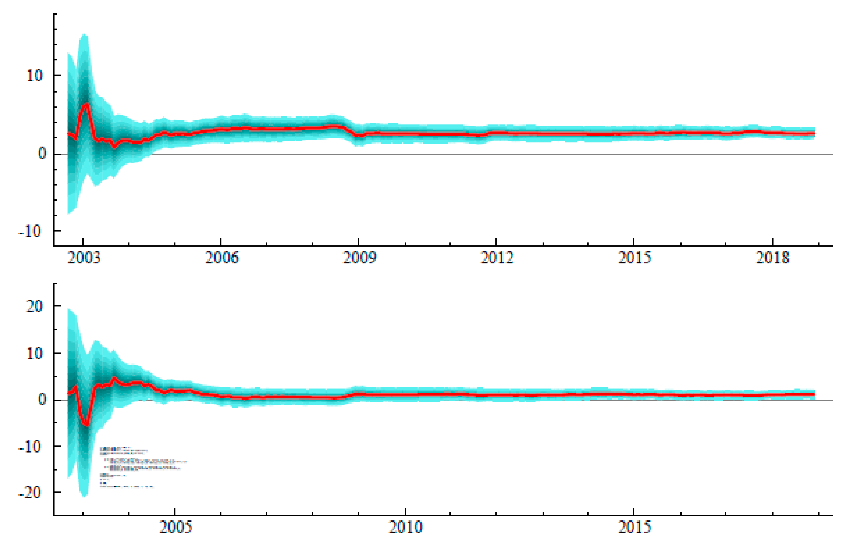
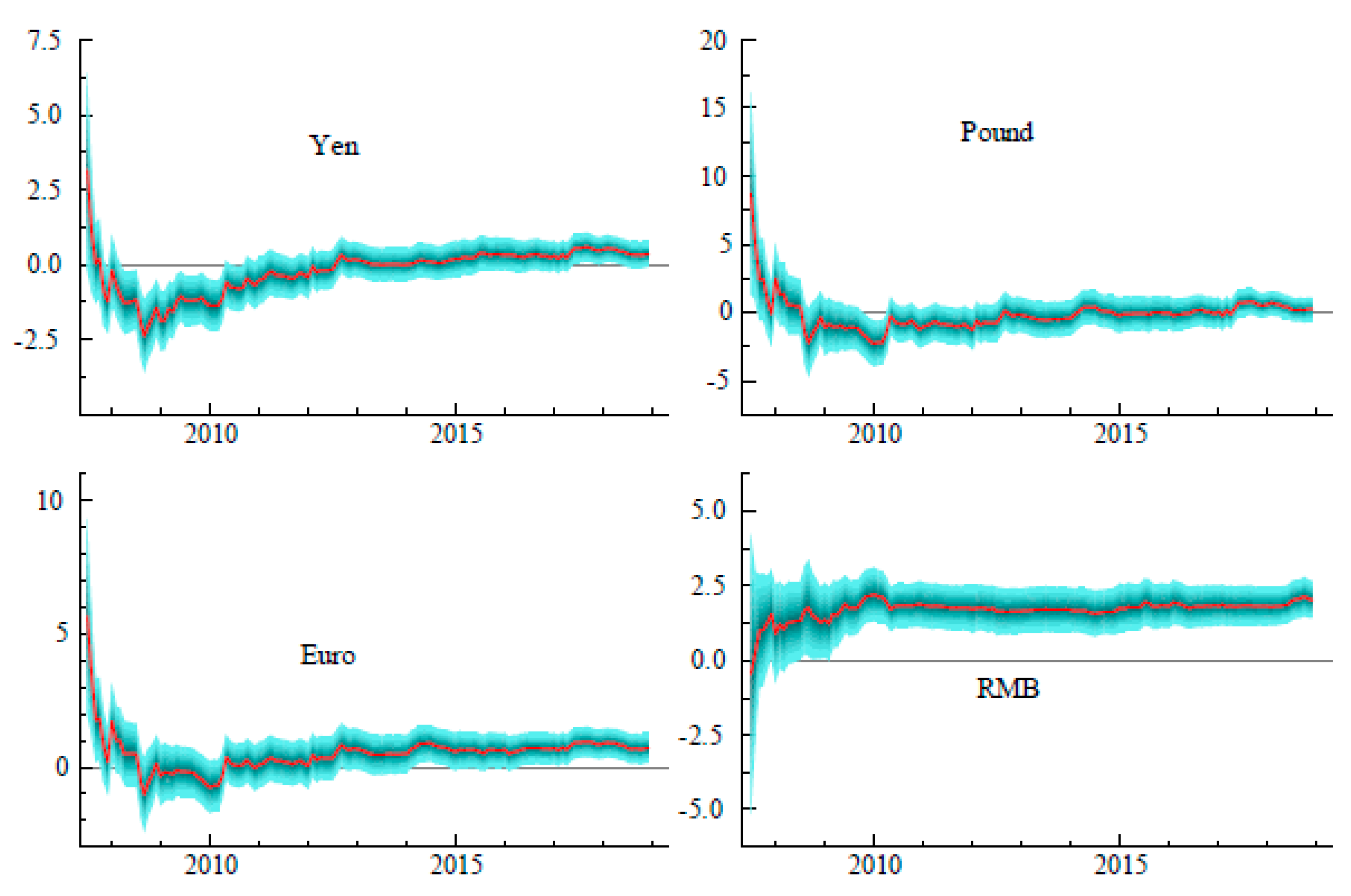
Parameter Constancy. To assess the assumed parameter constancy, we estimate the βs recursively. We begin with an initial sample size and then increase that sample size one observation at a time. Figure 6, Figure 7 and Figure 8 show the recursive 95 percent confidence intervals for the estimated βs: All of the parameter estimates are consistent with their assumed constancy.21
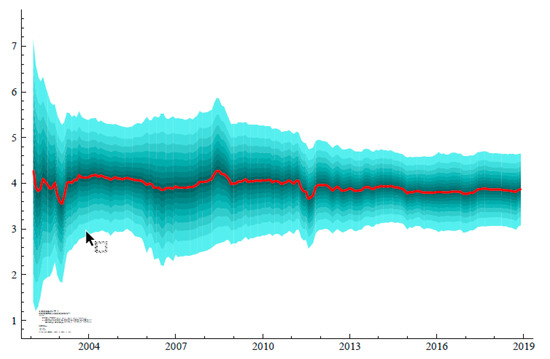
Figure 6.
Recursive Estimate of Coefficient for the Broad Real Effective Exchange Rate. Bands represent twice the standard deviation of the estimate.
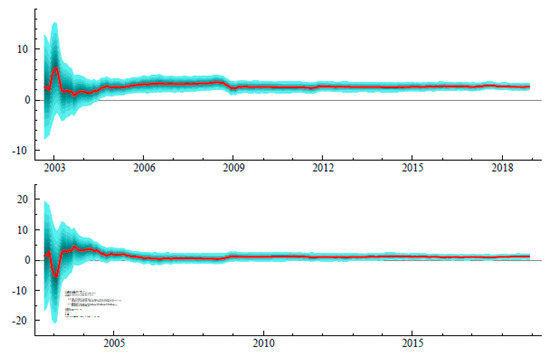
Figure 7.
Recursive Estimate of Coefficient for the Major (top panel) and Other Important Trading Partners (bottom panel) Real Effective Exchange Rates. Bands represent twice the standard deviation of the estimate.
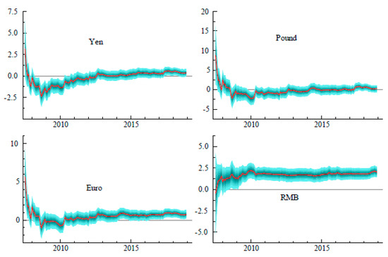
Figure 8.
Recursive Estimate of Coefficient for Bilateral Exchange Rates. Bands represent twice the standard deviation of the estimate.
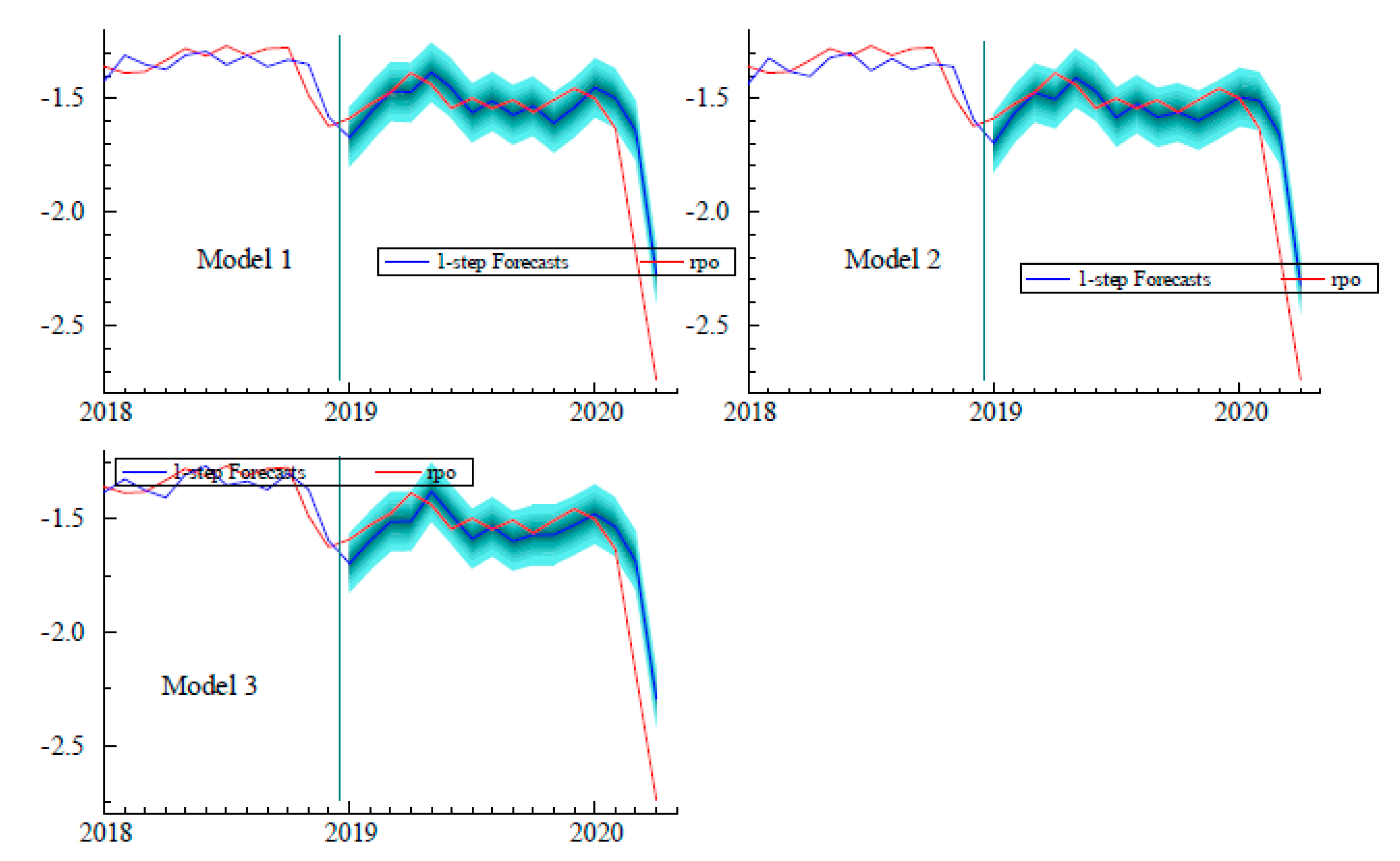
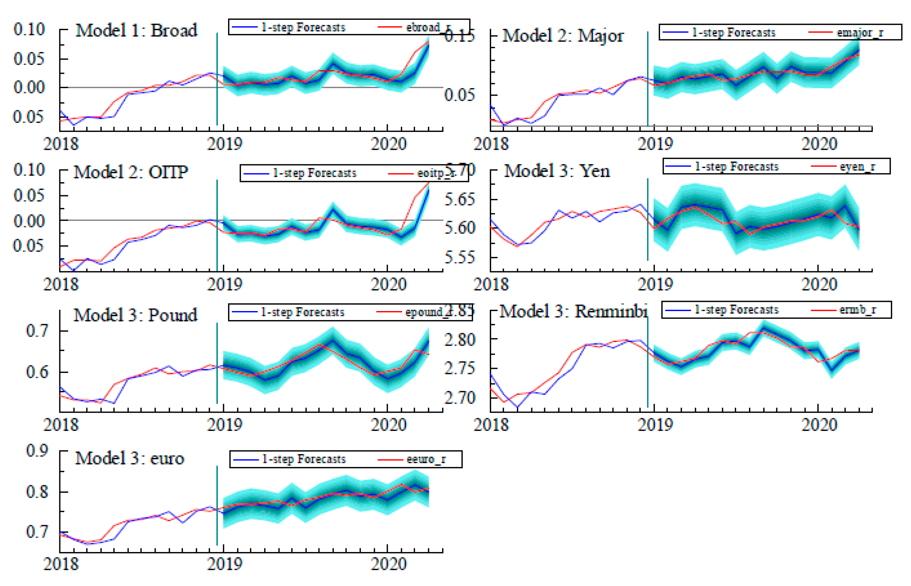
Predictive Accuracy. Projections for oil prices and bilateral exchange rates play a role in the formulation of U.S. monetary policy.22 However, for some practitioners, the pitfalls of real effective exchange rates might be acceptable if using them increases predictive accuracy. Figure 9 and Figure 10 show the 95 percent confidence bands of the models’ forecasts from January 2019 to April 2020.23
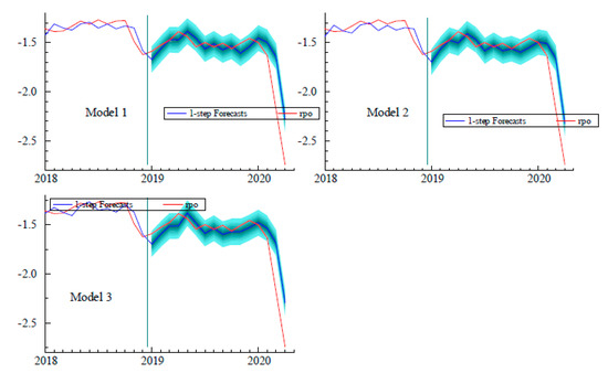
Figure 9.
Out-of-sample 1-step ahead forecasts for the real price of oil. Sensitivity to Model Specification.
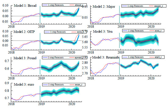
Figure 10.
Out-of-sample l-step ahead forecasts for exchange rates. Sensitivity to Model Specification.
Inspection of the results reveals several features of interest. First, the predictive accuracy for exchange rates of models using real effective exchange-rate indexes is worse than the predictive accuracy of the model based on bilateral rates. Indeed, the forecasts for model 3 show that the bilateral exchange rates are well within the 95 percent confidence bands, whereas the forecasts for models 1 and 2 are outside their bands starting in 2020. Second, the forecast for the real oil price is comparable across models: predictions are close to the actual price through February 2020. Third, the models show a significant decline in the predicted price of oil but not as large as the one observed in the market. As a result, there is a significant overprediction for March and April of 2020.
This overprediction is not likely to be the result of forecast errors in the exchange rates spilling over to the forecast for the price of oil. The prediction errors of the exchange-rate indexes cannot account for the nearly 50 percent overprediction of the price of oil in those models. Likely then, the overprediction for the price of oil is due to developments in the oil market as such. The models used here, however, cannot identify whether the decline in the price of oil owes to a contraction in oil demand, due to the contraction in economic activity, and/or to an expansion in oil supply, owing to the political tensions between Saudi Arabia and Russia during April 2020. Identifying the separate contributions involves using a structural Vector Autoregressive model such as the one developed by Kilian (2009) 24.
5. Conclusions
This paper offers an empirical characterization of the relation between the international price of oil and exchange rates that is both useful and reliable. Our characterization is useful because it rests on information about asset prices that are determined in functioning asset markets.25 Our characterization is reliable because its maintained assumptions are not rejected by the data. To be sure, our work has several limitations. First, the number of observations is not large, which means that both statistical estimates and forecast evaluation will benefit from expanding the sample. Second, using monthly observations limits the applicability of the findings to address high-frequency financial decisions. Until these, and other, limitations are addressed, the findings have an undeniably tentative character and need to be treated as preliminary ones.
Author Contributions
Conceptualization, J.M.; methodology, J.M.; investigation, J.M. and S.M.; data curation, S.M.; writing—original draft preparation, J.M.; writing—review and editing, J.M. All authors have read and agreed to the published version of the manuscript.
Funding
This research received no external funding.
Acknowledgments
We are truly grateful to four anonymous referees for several rounds of comments and to the editorial board.
Conflicts of Interest
The authors declare no conflict of interest.
Appendix A
Appendix A.1. Data Sources and Transformations
All the data come from the St. Louis Federal Reserve database Fred: https://fred.stlouisfed.org/Variables in upper case represent the mnemonics used in the Fred data base. Numerical entries represent the values of these variables in January 2000.
- d = log(TWEXBPA/99.84)
- dm = log(TWEXMPA/98.189)
- do = log(TWEXOPA/l10.784)
- p = po − pus
- po = log(MCOILWTICO
- pus = log(CPIAUCNS)
- = log(EXJPUS*CPIAUCNS/JPNCPIALLMINMEI
- = log((l/EXUSUK)*CPIAUCNS/CP0000GBM086NEST)
- = log(EXCHUS*CPIAUCNS/CHNCPIALLMINMEI)
- = log((l/EXUSEU)*CPIAUCNS/CP0000EZl9M086NEST)
- Nominal Yen/dollar DEXJPUS
- Nominal China: DEXCHUS
- Nominal Euro: DEXUSEU
- Nominal UK: DEXUSUK
- US CPI: CPIAUCNS
- Japanese CPI: JPNCPIALLMINMEI
- Chinese CPI: CHNCPIALLMINMEI
- euro CPI: CP0000EZ19M086NEST
- UK CPI CP0000GBM086NEST
Beginning in January of 2020, the Federal Reserve initiated a new weighting scheme which uses total trade, including oil. The revised series are indistinguishable from the series used in this paper. See von Beschwitz et al. (2019). For the new weights see https://www.federalreserve.gov/releases/h10/weights/default.htm
Appendix A.2. Augmented Dickey-Fuller Test Results
The equation for the augmented ADF test includes a constant and six lags of the change of the variable being examined.

Table A1.
Augmented Dickey Fuller Tests—1999:1–2020:4.
Table A1.
Augmented Dickey Fuller Tests—1999:1–2020:4.
| Levels of Logarithms | |||||||||
| ADF | (T = 249, Constant; 5% = −2.87, 1% = −3.46) | ||||||||
| Lag | £/$ | rmb/$ | €/$ | ¥/$ | D | Dm | Do | p | |
| 6 | −1.48 | −0.71 | −1.71 | −1.31 | −1.35 | −1.38 | −1.16 | −1.42 | |
| 5 | −1.58 | −0.81 | −1.60 | −1.38 | −1.31 | −1.33 | −1.15 | −1.50 | |
| 4 | −1.72 | −0.88 | −1.59 | −1.58 | −1.27 | −1.40 | −1.09 | −1.44 | |
| 3 | −1.67 | −0.91 | −1.50 | −1.71 | −1.15 | −1.15 | −1.11 | −1.51 | |
| 2 | −1.50 | −0.93 | −1.50 | −1.85 | −1.07 | −1.17 | −1.02 | −1.67 | |
| 1 | −1.39 | −0.97 | −1.63 | −1.66 | −1.30 | −1.31 | −1.25 | −1.59 | |
| 0 | −0.91 | −0.71 | −1.23 | −1.23 | −0.70 | −0.76 | −0.72 | −0.77 | |
| Difference of Logarithms | |||||||||
| (T = 248, Constant; 5% = −2.87, 1% = −3.46) | |||||||||
| Lag | ∆£/$ | ∆rmb/$ | ∆€/$ | ∆¥/$ | ∆D | ∆Dm | ∆Do | ∆p | |
| 6 | −6.414 ** | −6.307 ** | −5.771 ** | −6.602 ** | −5.996 ** | −6.050 ** | −5.630 ** | −4.956 ** | |
| 5 | −6.228 ** | −7.664 ** | −5.616 ** | −7.400 ** | −5.221 ** | −5.539 ** | −5.417 ** | −5.282 ** | |
| 4 | −6.472 ** | −7.144 ** | −6.450 ** | −7.944 ** | −5.754 ** | −6.118 ** | −5.886 ** | −5.164 ** | |
| 3 | −6.589 ** | −7.288 ** | −7.156 ** | −7.940 ** | −6.430 ** | −6.437 ** | −6.849 ** | −6.159 ** | |
| 2 | −7.479 ** | −7.816 ** | −8.663 ** | −8.282 ** | −7.920 ** | −8.474 ** | −7.658 ** | −6.614 ** | |
| 1 | −9.327 ** | −8.879 ** | −10.36 ** | −8.875 ** | −10.08 ** | −9.899 ** | −10.29 ** | −6.805 ** | |
| 0 | −12.65 ** | −10.24 ** | −12.19 ** | −12.25 ** | −10.47 ** | −11.28 ** | −10.66 ** | −9.471 ** | |
| Sample Statistics | |||||||||
| ∆£/$ | ∆rmb/$ | ∆€/$ | ∆¥/$ | ∆D | ∆Dm | ∆Do | ∆p | ||
| Monthly Growth Rates 1990:2−2020:4 255 Obs. | |||||||||
| Mean | 0.001 | −0.001 | 0.001 | 0.001 | 0.000 | 0.001 | 0.000 | −0.001 | |
| Std.Devn. | 0.021 | 0.010 | 0.023 | 0.023 | 0.012 | 0.016 | 0.011 | 0.098 | |
| Skewness | 0.400 | 0.086 | −0.080 | −0.030 | 0.438 | −0.113 | 1.329 | −1.799 | |
| Excess Kurtosis | 1.143 | 0.690 | 0.429 | 0.596 | 1.653 | 0.590 | 4.923 | 7.329 | |
| Minimum | −0.057 | −0.033 | −0.068 | −0.073 | −0.034 | −0.048 | −0.032 | −0.561 | |
| Maximum | 0.077 | 0.035 | 0.070 | 0.072 | 0.056 | 0.058 | 0.062 | 0.210 | |
| Median | 0.000 | −0.001 | 0.001 | 0.000 | 0.000 | 0.002 | −0.001 | 0.013 | |
| Normality | test (p-val) | 0.0018 ** | 0.0432 * | 0.211 | 0.082 | 0.0000 ** | 0.082 | 0.0000 ** | 0.0000 ** |
Note: * significant at the 5% significance level, ** significant at the 1% significance level.
References
- Amano, Robert, and Simon van Norden. 1998. Oil Prices and the Rise and Fall of the US Real Exchange Rate. Journal of International Money and Finance 17: 299–316. [Google Scholar] [CrossRef]
- Beckmann, Joscha, Robert Czudaj, and Vipin Arora. 2017. The Relationship between Oil Prices and Exchange Rates: Theory and Evidence; EIA Working Paper Series; Washington, DC: EIA, June.
- Benassy-Quere, Aganes, Valerie Mignon, and Alexis Penot. 2005. China and the Relationship between the Oil Price and the Dollar. CEPII Working Paper No 2005–16. Paris: CEPII, October. [Google Scholar]
- Breitenfellner, Andreas, and Jesus Crespo Cuaresma. 2008. Crude Oil Prices and the USD/EUR Exchange Rate. In Monetary Policy and the Economy. Wien: Oesterreichische Nationalbank (Austrian Central Bank), Q4/08, OeNB. pp. 102–21. [Google Scholar]
- Cheng, Kevin. 2008. Dollar Depreciation and Commodity Prices. In World Economic Outlook. Washington, DC: IMF, chp. 3. [Google Scholar]
- Doornik, Jurgen, and David Hendry. 2013. Empirical Econometric Modeling Vols. I and II. London: Timberlake Consultants. [Google Scholar]
- Federal Reserve Bank of New York. 2020. Oil Price Dynamics Report. Available online: https://www.newyorkfed.org/research/policy/oil_price_dynamics_report.html (accessed on 23 July 2020).
- Fratzscher, Marcel, Daniel Schneider, and Ine van Robays. 2014. Oil Prices, Exchange Rates and Asset Prices. ECB Working Paper l689. Frankfurt: ECB, July. [Google Scholar]
- Golub, Stephen. 1983. Oil Prices and Exchange Rates. Economic Journal 93: 576–93. [Google Scholar] [CrossRef]
- Grisse, Christian. 2010. What Drives the Oil-Dollar Correlation? New York: Federal Reserve Bank of New York. [Google Scholar]
- Huang, Bwo-Nung, Chi-Chuan Lee, Yu-Fang Chang, and Chien-Chiang Lee. 2020. Dynamic Linkage Between Oil Prices and Exchange Rates: New Global Evidence. Empirical Economics April. [Google Scholar] [CrossRef]
- Johansen, Soren. 1988. Statistical Analysis of Cointegration Vectors. Journal of Economic Dynamics and Control 12: 231–54. [Google Scholar]
- Kilian, Lutz. 2009. Not all oil price shocks are alike: Disentangling Demand and Supply Shocks in the Crude Oil Market. American Economic Review 99: 1059–69. [Google Scholar] [CrossRef]
- Krugman, Paul. 1980. Oil and the Dollar. NBER Working Paper No. 554. Cambridge: NBER. [Google Scholar]
- Leahy, Michael P. 1998. New Summary Measures of the Foreign Exchange Value of the Dollar; Washington, DC: Federal Reserve Bulletin, October.
- Reboredo, Juan, Miguel Rivera-Castro, and Gilney Zebende. 2014. Oil and US Dollar Exchange-rate Dependence: A Detrended Cross-correlation Approach. Energy Economics 42: 132–39. [Google Scholar] [CrossRef]
- Truman, Edwin. 2019. Federal Reserve Board Oral History Project: Interview with Edwin Truman. Available online: https://www.federalreserve.gov/aboutthefed/files/edwin-m-truman-interview-20091130.pdf (accessed on 23 July 2020).
- von Beschwitz, Bastian, Christopher Collins, and Deepa Datta. 2019. Revisions to the Federal Reserve Dollar Indexes. Available online: https://www.federalreserve.gov/econres/notes/feds-notes/revisions-to-the-federal-reserve-dollar-indexes-20190115.htm (accessed on 23 July 2020).
- Yousefi, Ayoub, and Tony S. Wirjanto. 2005. A Stylized Exchange Rate Pass-through Model of Crude Oil Price Formation. OPEC Review 29: 177–87. [Google Scholar] [CrossRef]
| 1. | For an early treatment of oil as a financial asset, see Fratzscher et al. (2014). |
| 2. | As noted in the June 2020 Monetary Policy Report of the Federal Reserve, “On April 20, the price of front-month oil futures contracts for West Texas Intermediate (WTI) closed at negative $38 per barrel. These WTI futures contracts are settled by physical delivery; as worries about the lack of available storage space intensified, prices spiraled downward. Few contracts were actually traded at these negative prices, and prices recovered in the following days.” See https://www.federalreserve.gov/monetarypolicy/files/202006l2_mprfullreport.pdf. |
| 3. | For a recent and thorough review of this literature see Beckmann et al. (2017). |
| 4. | More than 90 percent of international foreign exchange reserves are held in assets denominated in these currencies. See the IMF’s Currency Composition of Official Foreign Exchange Reserves. In terms of the global oil market, these five countries account for 55 percent of world oil consumption in 2019. |
| 5. | A switch to daily data would preclude measuring the variables in real terms because there are no official data for daily CPIs. |
| 6. | Breitenfellner and Cuaresma (2008) trace the origins of this relation. |
| 7. | Using PPP exchange rates. See the IMF’s World Economic Outlook. |
| 8. | Important exceptions are Benassy-Quere et al. (2005), Cheng (2008), and Huang et al. (2020). |
| 9. | Important exceptions are Amano and van Norden (1998), and Yousefi and Wirjanto (2005). |
| 10. | We are using the U.S. official measure of the external value of the dollar which uses weights that are updated every year. The measures of the IMF and the BIS update their weights with less frequency. See Truman (2019, pp. 126–31) for the history of this index. |
| 11. | Appendix A.1 contains all the data sources and transformations used in this paper. |
| 12. | In this sense, D is unlike the CPI in which the weights do not change from year to year. The obvious solution to this limitation is to use an effective exchange rate in which the weights do not vary from year to year as the indexes from the IMF and the BIS. Nevertheless, even if the weights were literally fixed, the reliance on the resulting aggregates still requires us to assume the existence of a market for D and would not remove the identification issues raised above. |
| 13. | Specifically, the 2020 weights for Russia and Saudi Arabia, two large oil producers are 0.53 percent and 0.49 percent, respectively. See https://www.federalreserve.gov/releases/hl0/weights/default.htm. |
| 14. | Note that using fixed weights would address that issue but it would not provide a financial market for the "fixed-weight external value of the dollar.” Further, movements in a fixed-weight index cannot, by construction, identify which currencies are responsible for those movements. |
| 15. | One of the referees noted that one could use the volatility spillover measure. This suggestion reinforces the point of the paper about using bilateral exchange rates. The volatility of the effective exchange rates is not meaningful, given that offsetting changes in exchange rates would induce a seemingly stable average. |
| 16. | Following the suggestion of one of the referees, the intercept c is included in the cointegration vector . |
| 17. | Indeed, the Euro area and China are the largest oil consumers (after the United States) and account for 29 percent of world oil consumption in 2019; if we include both Japan and the United Kingdom, that share increases to 34 percent. Source: International Energy Agency as reported in https://en.wikipedia.org/wiki/List_of_countries_by_oil_consumption. |
| 18. | Again, note that this equation is not determining p in terms of or the other way around. Instead, it is showing the relation among five endogenous variables that is consistent with no-arbitrage relation in these markets. In response to a shock, all the variables in the model respond according to Equation (1). These responses stop as soon as arbitrage opportunities are fully exploited. |
| 19. | For example, based on the IMF’s COFER data, the euro accounts for 20 percent of the world’s official foreign exchange reserves, whereas the renminbi accounts for 2 percent. Using an alternative indicator, the turnover of OTC foreign exchange instruments in 2019 for the euro is $2.l trillion and $285 billion dollars for the renminbi. See https://stats.bis.org/statx/srs/table/dll.3. |
| 20. | These observations benefited greatly from the comments by a referee. |
| 21. | We could not reject dynamic stability based on impulse responses. These results are available on request. |
| 22. | See the Minutes of the Federal Open Market Committee from May 2020 at https://www.federalreserve.gov/monetarypolicy/files/fomcminutes20200429.pdf. Further, the Federal Reserve Bank of New York’s Oil Price Dynamics Report does not rely on effective exchange rates but instead on bilateral rates (Federal Reserve Bank of New York 2020). |
| 23. | The estimation sample ends in December 20l8, meaning that forecasts are based on those estimates without further update. The “one-step-ahead” refers to the practice of financial forecasters of starting their forecasts from the most recent data. As for the length of the horizon, one year is arbitrary but it is the horizon over which analysts focus, such as the Federal Reserve Bank of New York’s Oil-price Dynamics Report. |
| 24. | We appreciate the comments from a referee on the lack of identification associated with our model. |
| 25. | For example, one could combine futures and options contracts. The futures contract would be for a given price of oil; the option contract would have strike prices determined by a long-run relation between the price of oil and the dollar. Moreover, the Federal Reserve Bank of New York releases its weekly analysis of the price of oil and they use bilateral exchange rates. |
© 2020 by the authors. Licensee MDPI, Basel, Switzerland. This article is an open access article distributed under the terms and conditions of the Creative Commons Attribution (CC BY) license (http://creativecommons.org/licenses/by/4.0/).

