Modelling Returns in US Housing Prices—You’re the One for Me, Fat Tails
Abstract
1. Introduction
2. Related Literature
3. Data
4. Methodological Framework
5. Empirical Analysis
5.1. Within-Sample Estimation Results
5.2. Out-of-Sample Analysis
5.3. Discussion of the Results
6. Conclusions
Author Contributions
Funding
Institutional Review Board Statement
Informed Consent Statement
Data Availability Statement
Acknowledgments
Conflicts of Interest
Appendix A
| (1) | (2) | (3) | (4) | (5) | ||
|---|---|---|---|---|---|---|
| Mean equation [AR(5)] | 0.028 | 0.031 | 0.033 | 0.028 | 0.026 | |
| (0.032) | (0.003) | (0.000) | (0.004) | (0.010) | ||
| 1.909 | 1.970 | 1.937 | 1.970 | 1.970 | ||
| (0.000) | (0.000) | (0.000) | (0.000) | (0.000) | ||
| −0.919 | −0.897 | −0.838 | −0.909 | −0.915 | ||
| (0.000) | (0.000) | (0.000) | (0.000) | (0.000) | ||
| −0.234 | −0.469 | −0.538 | −0.454 | −0.438 | ||
| (0.018) | (0.000) | (0.000) | (0.000) | (0.000) | ||
| 0.430 | 0.640 | 0.717 | 0.638 | 0.627 | ||
| (0.000) | (0.000) | (0.000) | (0.000) | (0.000) | ||
| −0.192 | −0.249 | −0.284 | −0.250 | −0.248 | ||
| (0.000) | (0.000) | (0.000) | (0.000) | (0.000) | ||
| GARCH equation | 0.001 | 0.001 | 0.001 | 0.001 | ||
| (0.003) | (0.010) | (0.008) | (0.006) | |||
| 0.215 | 0.124 | 0.192 | 0.188 | |||
| (0.000) | (0.001) | (0.000) | (0.000) | |||
| 0.742 | 0.724 | 0.759 | 0.762 | |||
| (0.000) | (0.000) | (0.000) | (0.000) | |||
| Degrees of freedom | 6.734 | 6.958 | ||||
| [1.948] | [2.020] | |||||
| Skewness parameter | −0.065 | |||||
| (0.283) | ||||||
| ARCH-test | 115.610 | 8.634 | 8.082 | 8.094 | 8.032 | |
| (0.000) | (0.734) | (0.778) | (0.777) | (0.783) | ||
| JB-test | 1817.200 | 49.303 | 9.748 a | 1.758 a | 0.201 a | |
| (0.000) | (0.000) | (0.008) | (0.415) | (0.904) | ||
| N | 537 | 537 | 537 | 537 | 537 |
Appendix B
| Mean | Variance | Skewness | Kurtosis | Jarque–Bera | ADF | KPSS | N |
|---|---|---|---|---|---|---|---|
| 0.739 | 18.405 | −0.246 | 3.757 | 26.785 | −3.322 | 0.149 | 789 |
| Normal distribution | 0.010 | 3.449 | 1.706 | 2.022 | 1.011 | 1.011 |
| 0.025 | 2.906 | 1.706 | 1.704 | 0.852 | 0.852 | |
| 0.050 | 2.439 | 1.706 | 1.430 | 0.715 | 0.715 | |
| Unconditional returns | 0.010 | 4.423 | 1.784 | 2.479 | 1.103 | 1.375 |
| 0.025 | 3.413 | 1.784 | 1.913 | 1.003 | 0.910 | |
| 0.050 | 2.795 | 1.784 | 1.566 | 0.815 | 0.751 |
| (1) | (2) | (3) | (4) | (5) | ||
|---|---|---|---|---|---|---|
| Mean equation [AR(5)] | 0.010 | 0.022 | 0.023 | 0.023 | 0.023 | |
| (0.524) | (0.134) | (0.000) | (0.092) | (0.106) | ||
| 1.392 | 1.407 | 1.409 | 1.419 | 1.419 | ||
| (0.000) | (0.000) | (0.000) | (0.000) | (0.000) | ||
| −0.328 | −0.352 | −0.316 | −0.364 | −0.364 | ||
| (0.000) | (0.000) | (0.000) | (0.000) | (0.000) | ||
| −0.078 | −0.069 | −0.097 | −0.070 | −0.069 | ||
| (0.231) | (0.283) | (0.000) | (0.294) | (0.297) | ||
| 0.103 | 0.102 | 0.069 | 0.106 | 0.105 | ||
| (0.100) | (0.098) | (0.001) | (0.094) | (0.085) | ||
| −0.101 | −0.100 | −0.077 | −0.102 | −0.102 | ||
| (0.005) | (0.005) | (0.000) | (0.005) | (0.004) | ||
| GARCH equation | 0.003 | 0.002 | 0.003 | 0.003 | ||
| (0.078) | (0.180) | (0.158) | (0.158) | |||
| 0.087 | 0.077 | 0.105 | 0.105 | |||
| (0.000) | (0.001) | (0.000) | (0.000) | |||
| 0.898 | 0.859 | 0.886 | 0.886 | |||
| (0.000) | (0.000) | (0.000) | (0.000) | |||
| Degrees of freedom | 9.672 | 9.676 | ||||
| [2.882] | [3.810] | |||||
| Skewness parameter | 0.004 | |||||
| (0.080) | ||||||
| ARCH-test | 96.036 | 29.762 | 28.187 | 28.455 | 28.439 | |
| (0.000) | (0.003) | (0.005) | (0.005) | (0.005) | ||
| JB-test | 11.867 | 20.310 | 17.761 a | 0.105 a | 0.067 a | |
| (0.006) | (0.000) | (0.000) | (0.949) | (0.967) | ||
| N | 789 | 789 | 789 | 789 | 789 |
| RMSE | DM | KS | AD | KL | |
|---|---|---|---|---|---|
| Normal—Homoscedastic | 0.435 | - | 0.093 | 5.419 | 0.038 |
| Normal—GARCH | 0.432 | 1.864 | 0.065 | 2.501 | 0.021 |
| Laplace—GARCH | 0.434 | 0.183 | 0.112 | 14.240 | 0.068 |
| Student-t—GARCH | 0.431 | 2.003 | 0.058 | 2.152 | 0.015 |
| Skew-t—GARCH | 0.431 | 2.007 | 0.060 | 2.070 | 0.016 |
| 1 | The real prices are Shiller’s (2015); the CPI has been used as the deflator. As can be seen when comparing our main results to those in Appendix B, the results using real returns are qualitatively similar. Most importantly, we found that the Student-t GARCH and Skew-t GARCH specifications are the only ones whose residuals pass the Jarque–Bera test for normality. These two models also have the best out-of-sample forecast performance. |
| 2 | The measures are related to each other and the quantiles of the distribution by the formula
|
| 3 | Fagiolo et al. (2008) found the Laplace distribution useful when modelling the fat tails of GDP growth rates. The Student-t distribution has been used more widely in the empirical literature; see, for example, Cúrdia et al. (2014); Clark and Ravazzolo (2015); Cross and Poon (2016); and Kiss and Österholm (2020). |
| 4 | |
| 5 | As pointed out by Diebold (2015), the Diebold and Mariano (1995) test in its standard form is a reasonable choice even if we employ nested models, for which the original assumptions of the test do not formally hold. This is further supported by the fact that the test performs relatively well in such larger training and evaluation samples as the one we use in our analysis (Clark and McCracken 2013). |
| 6 | The KL divergence has been used in a number of applications in the context of density forecasts—typically though with a somewhat different focus; see, for example, Cogley et al. (2005); Robertson et al. (2005); Hall and Mitchell (2007); Diks et al. (2010) and Mitchell and Wallis (2011). |
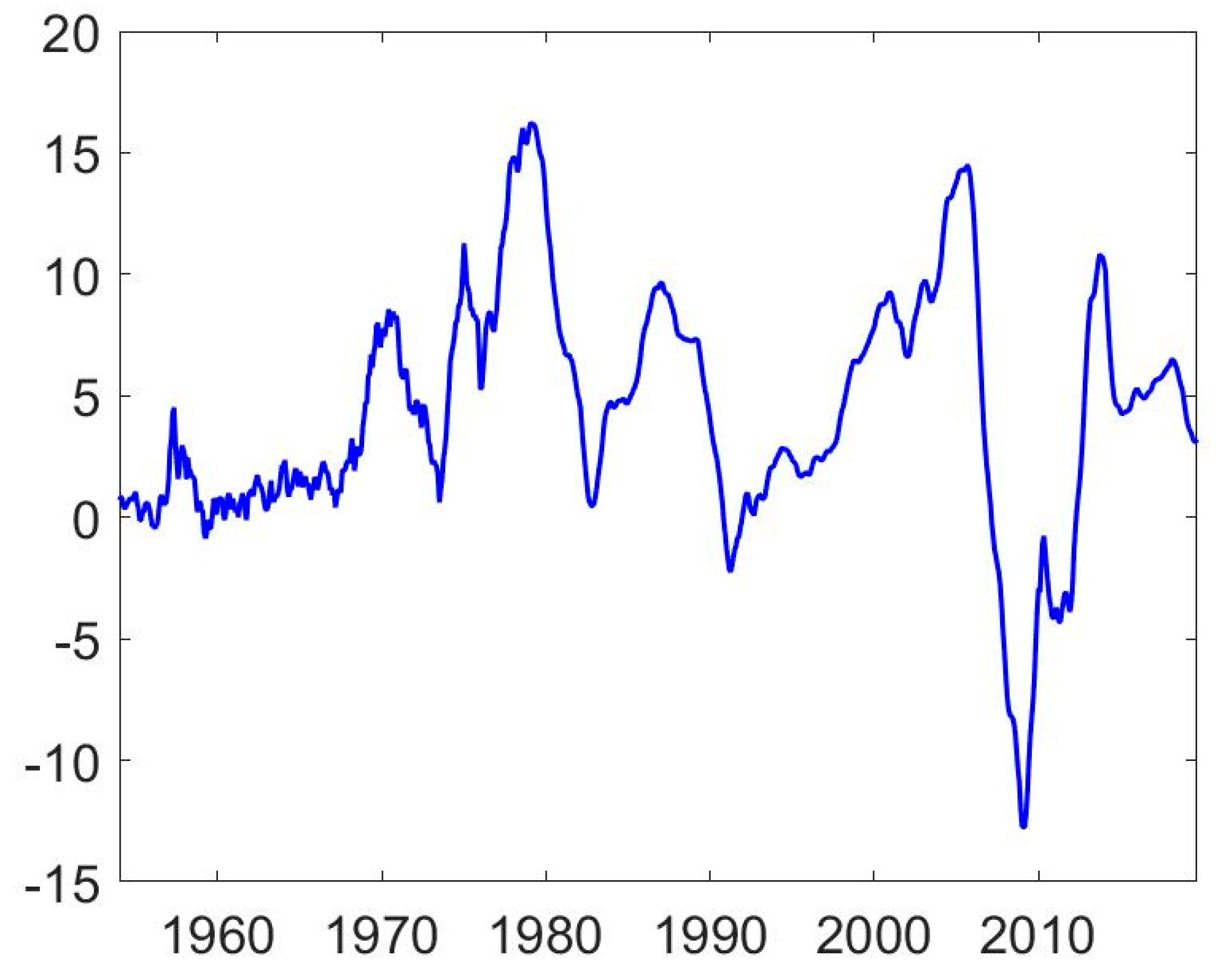
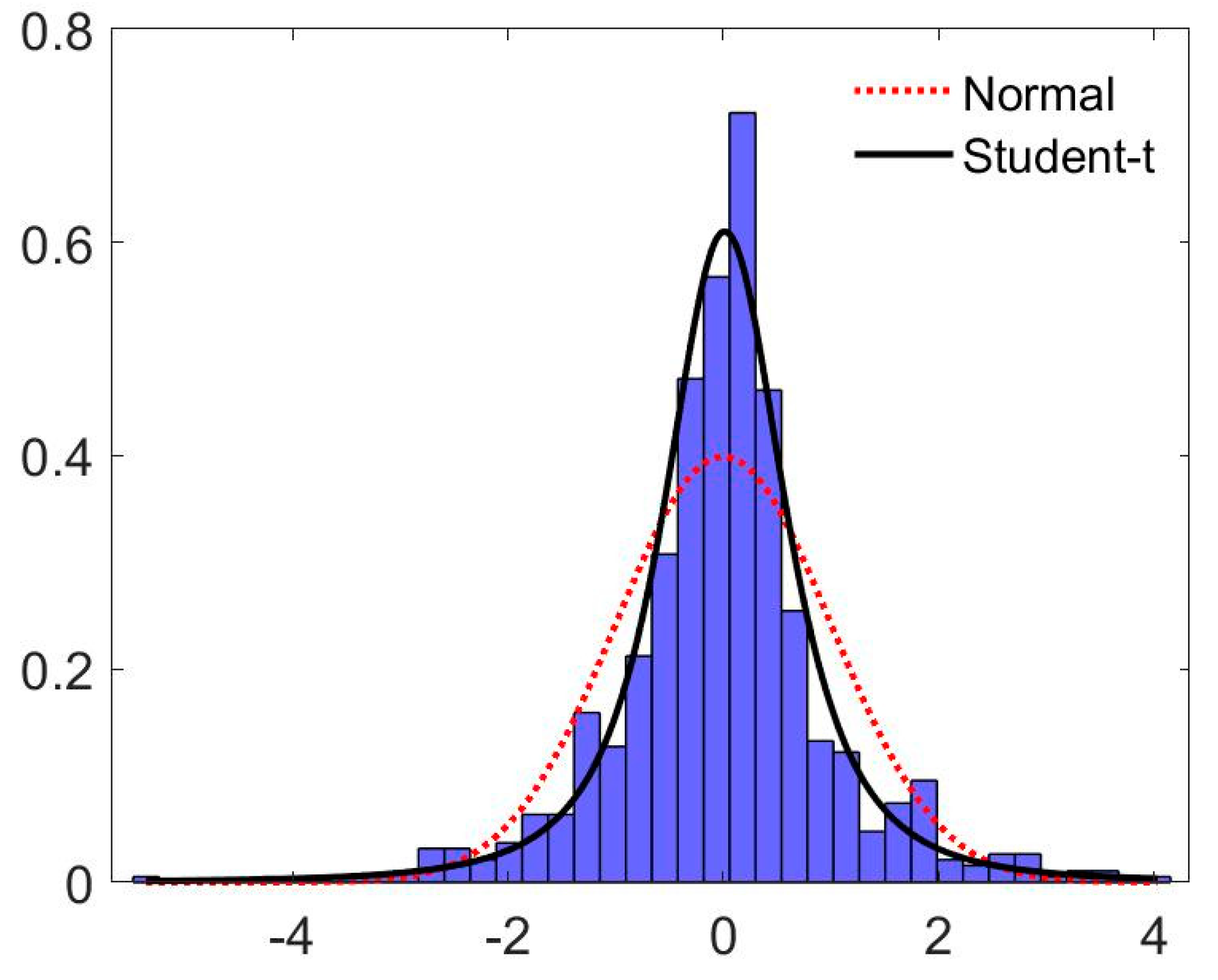
| 7 | Figure 1 suggests that the time-series behaviour of the return series may have changed around 1975. In fact, the Shiller (2015) dataset changes source in January 1975. Therefore, we also estimate the model on the shorter subsample, namely, January 1975 to September 2019. The results collected in Table A1 in Appendix A are qualitatively very similar to full sample estimates. |
| 8 | We also assessed the robustness of our results to the presence of different regimes, in particular the boom and bust cycle between 2002 and 2009. We did this by allowing for a different constant and dynamics in the mean equation during this period, using a time dummy and interactions. Unreported results (available upon request from the authors) show very similar results to our baseline. Capturing non-Gaussianity in the innovations remains a salient and important feature of the model. |
| 9 | In fact, the parameters and sum up to unity for the normal-GARCH, Student-t-GARCH and Skew-t-GARCH specifications. However, looking at the results using the Laplace distribution and the shorter sample, integrated volatility does not seem to be a robust feature of the data, therefore we do not impose it in any of the specifications with conditional heteroscedasticity. |
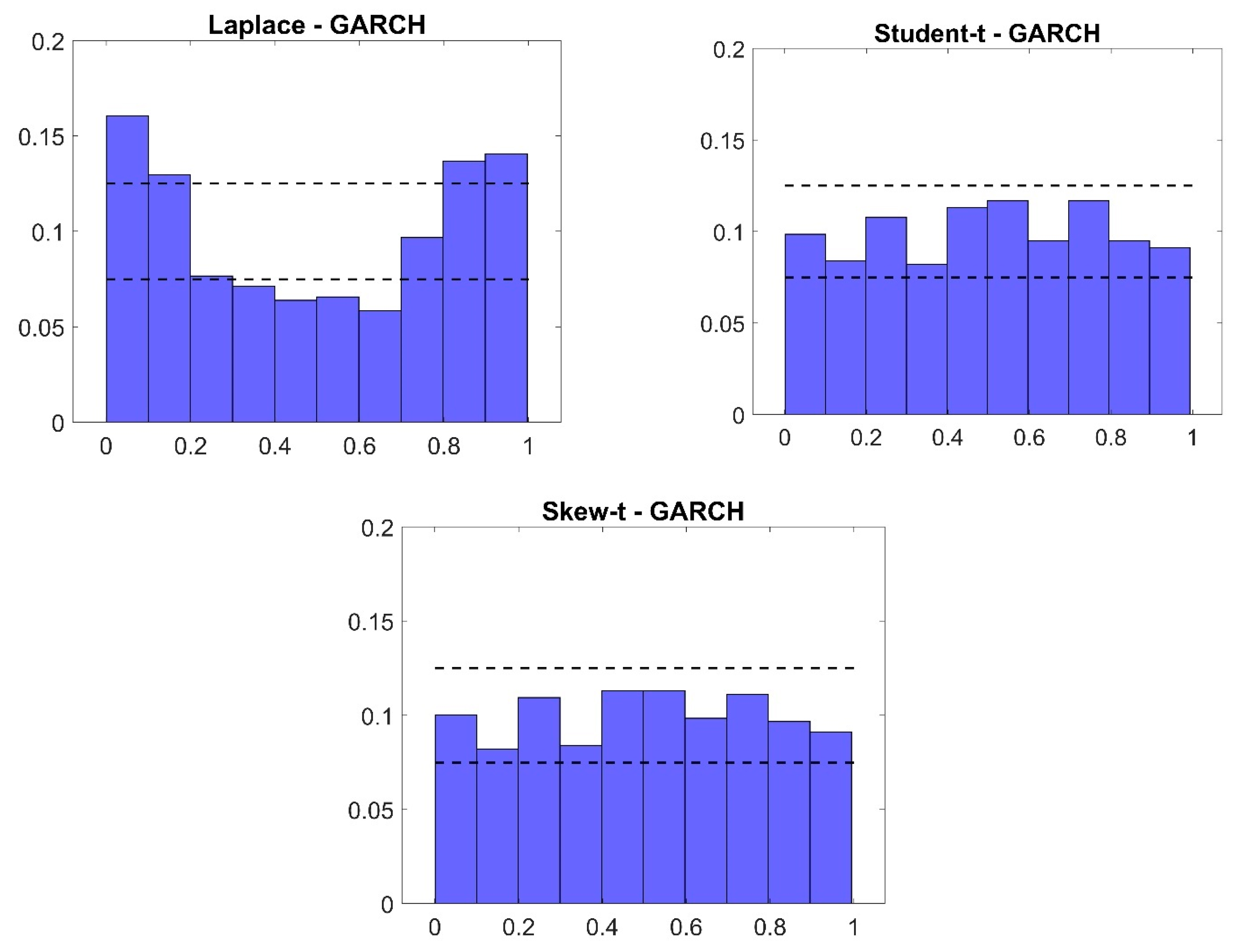
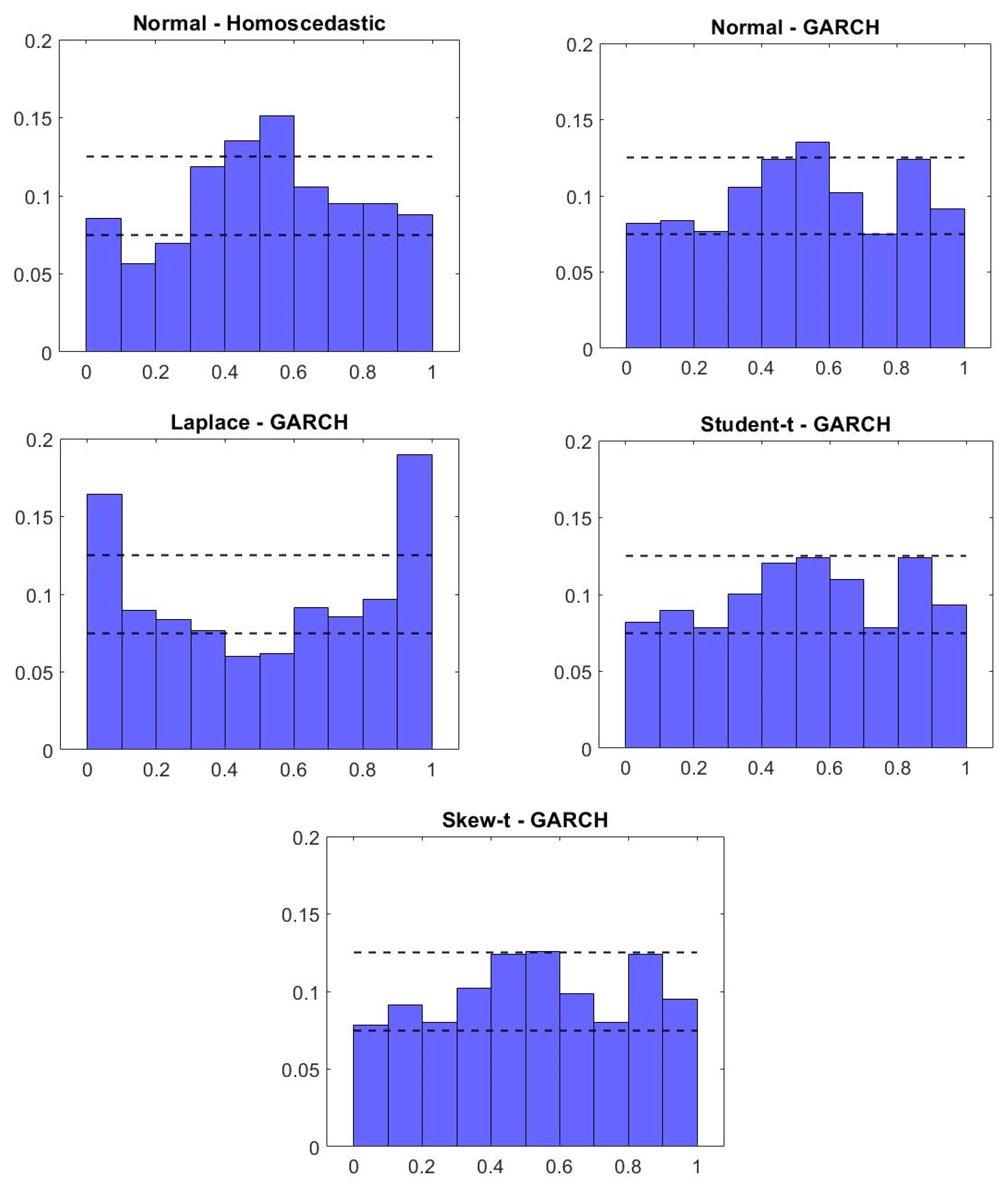
| 10 | The Jarque–Bera tests are based on , the PIT series of the standardised residuals, for which is standard normally distributed (where is the inverse cumulative distribution function of the standard normal distribution). We test this by applying the Jarque–Bera test on . |
| 11 | That is, we first estimate the models on the sample January 1953 to January 1974 and make predictions for February 1974. We then expand the sample to January 1953 to February 1974, re-estimate the models and predict March 1974. We continue in this manner until we reach the end of the sample, where we estimate the models using data from January 1953 to August 2019 and make predictions for September 2019. |
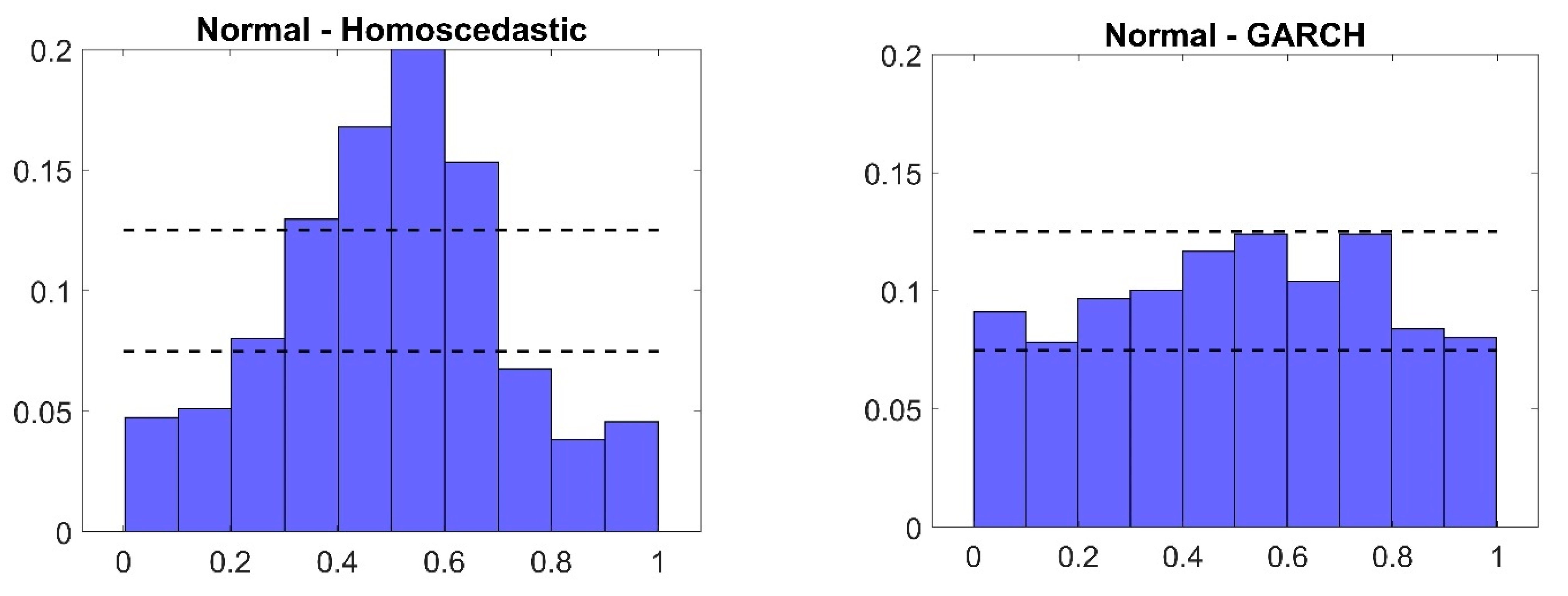
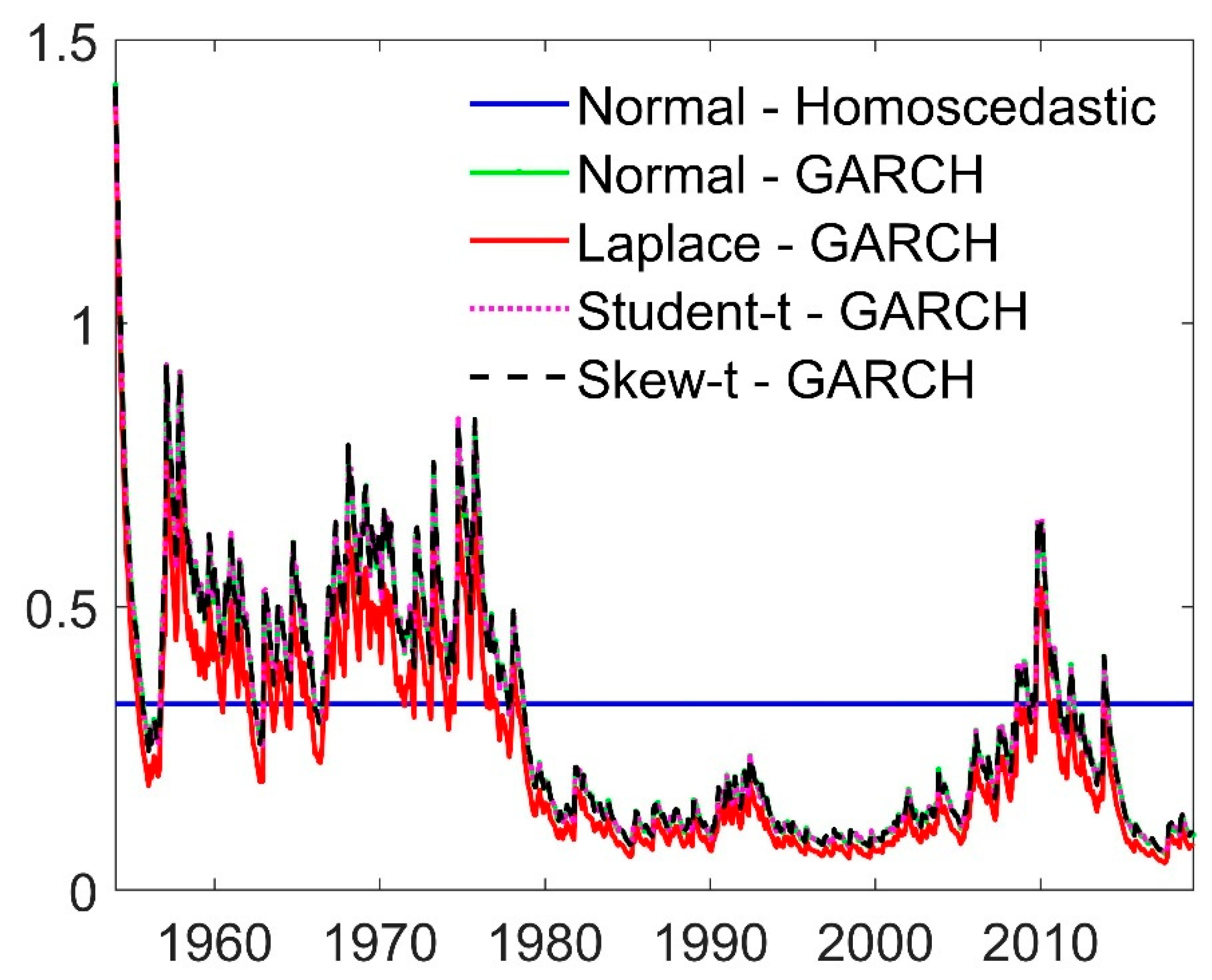
| 12 | This finding is concordant with the fact that our within-sample analysis indicates that the unconditional volatility overestimates the conditional one in the larger part of the out-of-sample evaluation period; see Figure 4. |
| 13 | Non-Gaussianity is also important for identifying a housing-price shock in a VAR model. Lanne et al. (2017) show that it is possible to identify an otherwise unidentified structural VAR model by deviating from the Gaussian assumption. That helps solve the problem discussed in Musso et al. (2011), namely, that housing-price shocks are not identified in a VAR model with Gaussian error terms. |
References
- Acemoglu, Daron, and Andrew Scott. 1997. Asymmetric business cycles: Theory and time-series evidence. Journal of Monetary Economics 40: 501–33. [Google Scholar] [CrossRef]
- Acolin, Arthur. 2020. Housing wealth and consumption over the 2001–2013 period: The role of the collateral channel. Journal of Housing Research 29: 68–88. [Google Scholar] [CrossRef]
- Adrian, Tobias, Federico Grinberg, Nellie Liang, and Shehereya Malik. 2018. The Term Structure of Growth-at-Risk. Working Paper 18/180. Washington, DC, USA: International Monetary Fund. [Google Scholar]
- Adrian, Tobias, Nina Boyarchenko, and Domenico Giannone. 2019. Vulnerable growth. American Economic Review 109: 1263–89. [Google Scholar] [CrossRef]
- Ahamada, Ibrahim, and Jose Luis Diaz Sanchez. 2013. A Retrospective Analysis of the House Prices Macro-Relationship in the United States. World Bank Policy Research Working Paper 6549. Available online: https://ssrn.com/abstract=2303105 (accessed on 15 July 2021).
- Anderson, Theodore W., and Donald A. Darling. 1952. Asymptotic theory of certain goodness of fit criteria based on stochastic processes. Annals of Mathematical Statistics 23: 193–212. [Google Scholar] [CrossRef]
- Ascari, Guido, Giorgio Fagiolo, and Andrea Roventini. 2015. Fat-tail distributions and business-cycle models. Macroeconomic Dynamics 19: 465–76. [Google Scholar] [CrossRef]
- Bekaert, Geert, and Alexander Popov. 2019. On the link between the volatility and skewness of growth. IMF Economic Review 67: 746–90. [Google Scholar] [CrossRef]
- Bollerslev, Tim. 1986. Generalized autoregressive conditional heteroskedasticity. Journal of Econometrics 31: 307–27. [Google Scholar] [CrossRef]
- Campbell, John Y., and Joao F. Cocco. 2007. How do house prices affect consumption? Evidence from micro data. Journal of Monetary Economics 54: 591–621. [Google Scholar] [CrossRef]
- Case, Karl E., and Robert J. Shiller. 1989. The efficiency of the market for single-family homes. The American Economic Review 79: 125–37. [Google Scholar]
- Catte, Pietro, Nathalie Girouard, Robert Price, and Christophe André. 2004. Housing Markets, Wealth and the Business Cycle. OECD Economics Working Paper 394. Available online: https://doi.org/10.1787/534328100627 (accessed on 15 May 2021).
- Chiang, Ming-Chu, I-Chun Tsai, and Cheng-Feng Lee. 2012. The Downside Risk of US and UK Housing Markets. Journal of Real Estate Portfolio Management 18: 257–72. [Google Scholar] [CrossRef]
- Chung, Hess, Jean-Philippe Laforte, David Reifschneider, and John C. Williams. 2012. Have we underestimated the likelihood and severity of zero lower bound events? Journal of Money, Credit and Banking 44: 47–82. [Google Scholar] [CrossRef]
- Clark, Todd E., and Michael McCracken. 2013. Advances in forecast evaluation. In Handbook of Economic Forecasting. Edited by Graham Elliott and Allan Timmermann. Amsterdam: Elsevier, vol. 2, pp. 1107–201. [Google Scholar]
- Clark, Todd E., and Francesco Ravazzolo. 2015. Macroeconomic forecasting performance under alternative specifications of time-varying volatility. Journal of Applied Econometrics 30: 551–75. [Google Scholar] [CrossRef]
- Cogley, Timothy, and Thomas J. Sargent. 2005. Drifts and volatilities: Monetary policies and outcomes in the post WWII US. Review of Economic Dynamics 8: 262–302. [Google Scholar] [CrossRef]
- Cogley, Timothy, Sergei Morozov, and Thomas J. Sargent. 2005. Bayesian fan charts for UK inflation: Forecasting and sources of uncertainty in an evolving monetary system. Journal of Economic Dynamics and Control 29: 1893–925. [Google Scholar] [CrossRef]
- Cross, Jamie, and Aubrey Poon. 2016. Forecasting structural change and fat-tailed events in Australian macroeconomic variables. Economic Modelling 58: 34–51. [Google Scholar] [CrossRef]
- Cúrdia, Vasco, Marco Del Negro, and Daniel L. Greenwald. 2014. Rare shocks, great recessions. Journal of Applied Econometrics 29: 1031–52. [Google Scholar] [CrossRef]
- Diebold, Francis X. 2015. Comparing predictive accuracy, twenty years later: A personal perspective on the use and abuse of Diebold-Mariano tests. Journal of Business and Economic Statistics 33: 1–9. [Google Scholar] [CrossRef]
- Diebold, Francis X., and Robert S. Mariano. 1995. Comparing predictive accuracy. Journal of Business and Economic Statistics 13: 134–44. [Google Scholar]
- Diebold, Francis X., Todd A. Gunther, and Anthony S. Tay. 1998. Evaluating density forecasts with applications to financial risk management. International Economic Review 39: 863–83. [Google Scholar] [CrossRef]
- Diks, Cees, Valentyn Panchenko, and Dick Van Dijk. 2010. Out-of-sample comparison of copula specifications in multivariate density forecasts. Journal of Economic Dynamics and Control 34: 1596–609. [Google Scholar] [CrossRef][Green Version]
- Dufitinema, Josephine. 2021. Stochastic volatility forecasting of the Finnish housing market. Applied Economics 53: 98–114. [Google Scholar] [CrossRef]
- Engle, Robert F. 1982. Autoregressive conditional heteroscedasticity with estimates of the variance of United Kingdom inflation. Econometrica 50: 987–1007. [Google Scholar] [CrossRef]
- Fagiolo, Giorgio, Mauro Napoletano, and Andrea Roventini. 2008. Are output growth-rate distributions fat-tailed? Some evidence from OECD countries. Journal of Applied Econometrics 23: 639–69. [Google Scholar] [CrossRef]
- Faust, Jon, and Jonathan H. Wright. 2009. Comparing Greenbook and reduced form forecasts using a large realtime dataset. Journal of Business and Economic Statistics 27: 468–79. [Google Scholar] [CrossRef]
- Foster, Chester, and Robert Van Order. 1984. An option-based model of mortgage default. Housing Finance Review 3: 351. [Google Scholar]
- Graff, Richard, Adrian Harrington, and Michael Young. 1997. The shape of Australian real estate return distributions and comparisons to the United States. Journal of Real Estate Research 14: 291–308. [Google Scholar] [CrossRef]
- Granziera, Eleonora, and Sharon Kozicki. 2015. House price dynamics: Fundamentals and expectations. Journal of Economic Dynamics and Control 60: 152–65. [Google Scholar] [CrossRef]
- Hall, Stephen G., and James Mitchell. 2007. Combining density forecasts. International Journal of Forecasting 23: 1–13. [Google Scholar] [CrossRef]
- Hansen, Bruce E. 1994. Autoregressive conditional density estimation. International Economic Review 35: 705–30. [Google Scholar] [CrossRef]
- Hansen, Peter R., and Asger Lunde. 2005. A forecast comparison of volatility models: Does anything beat a GARCH (1, 1)? Journal of Applied Econometrics 20: 873–89. [Google Scholar] [CrossRef]
- Hjalmarsson, Erik, and Pär Österholm. 2020. Heterogeneity in households’ expectations of housing prices-evidence from micro data. Journal of Housing Economics 50: 101731. [Google Scholar] [CrossRef]
- Iacoviello, Matteo. 2005. House prices, borrowing constraints, and monetary policy in the business cycle. American Economic Review 95: 739–64. [Google Scholar] [CrossRef]
- Iacoviello, Matteo, and Stefano Neri. 2010. Housing market spillovers: Evidence from an estimated DSGE model. American Economic Journal: Macroeconomics 2: 125–64. [Google Scholar] [CrossRef]
- Jordá, Óscar, Katharina Knoll, Dmitry Kuvshinov, Mority Schularick, and Alan M. Taylor. 2019. The rate of return on everything, 1870–2015. Quarterly Journal of Economics 134: 1225–98. [Google Scholar] [CrossRef]
- Kiss, Tamás, and Pär Österholm. 2020. Fat tails in leading indicators. Economics Letters 193: 109317. [Google Scholar] [CrossRef]
- Klarl, Torben. 2016. The nexus between housing and GDP re-visited: A wavelet coherence view on housing and GDP for the US. Economics Bulletin 36: 704–20. [Google Scholar]
- Kullback, Solomon, and Richard A. Leibler. 1951. On information and sufficiency. Annals of Mathematical Statistics 22: 79–86. [Google Scholar] [CrossRef]
- Lanne, Markku, Mika Meitz, and Pentti Saikkonen. 2017. Identification and estimation of non-Gaussian structural vector autoregressions. Journal of Econometrics 196: 288–304. [Google Scholar] [CrossRef]
- Leung, Charles Ka Yui, Youngman Chun Fai Leong, and Siu Kei Wong. 2006. Housing price dispersion: An empirical investigation. Journal of Real Estate Finance and Economics 32: 357–85. [Google Scholar] [CrossRef]
- Liu, Xiaochun. 2019. On tail fatness of macroeconomic dynamics. Journal of Macroeconomics 62: 103154. [Google Scholar] [CrossRef]
- Ma, Chao. 2020. Momentum and reversion to fundamentals: Are they captured by subjective expectations of house prices? Journal of Housing Economics 49: 101687. [Google Scholar] [CrossRef]
- Martín-Legendre, Juan, Pablo Castellanos-García, and José Manuel Sánchez-Santos. 2019. Housing and financial wealth effects on consumption: Evidence from the Spanish Survey of Household Finances. Economics Bulletin 39: 1930–40. [Google Scholar]
- Maurer, Raimond, Frank Reiner, and Steffen P. Sebastian. 2004. Financial characteristics of international real estate returns: Evidence from the UK, US, and Germany. Journal of Real Estate Portfolio Management 10: 59–76. [Google Scholar]
- McMillan, David G. 2012. Long-run stock price-house price relation: Evidence from an ESTR model. Economics Bulletin 32: 1737–46. [Google Scholar] [CrossRef]
- Mitchell, James, and Kenneth F. Wallis. 2011. Evaluating density forecasts: Forecast combinations, model mixtures, calibration and sharpness. Journal of Applied Econometrics 26: 1023–40. [Google Scholar] [CrossRef]
- Musso, Alberto, Stefano Neri, and Livio Stracca. 2011. Housing, consumption and monetary policy: How different are the US and the euro area? Journal of Banking and Finance 35: 3019–41. [Google Scholar] [CrossRef]
- Myer, F. C. Neil, and James R. Webb. 1994. Statistical properties of returns: Financial assets versus commercial real estate. Journal of Real Estate Finance and Economics 8: 267–82. [Google Scholar] [CrossRef]
- Neftci, Salih N. 1984. Are economic time series asymmetric over the business cycle? Journal of Political Economy 92: 307–28. [Google Scholar] [CrossRef]
- Pan, Xuefeng, and Weixing Wu. 2021. Housing returns, precautionary savings and consumption: Micro evidence from China. Journal of Empirical Finance 60: 39–55. [Google Scholar] [CrossRef]
- Piazzesi, Monika, and Martin Schneider. 2009. Momentum traders in the housing market: Survey evidence and a search model. American Economic Review 99: 406–11. [Google Scholar] [CrossRef]
- Pontines, Victor. 2010. Fat-tails and house prices in OECD countries. Applied Economics Letters 17: 1373–77. [Google Scholar] [CrossRef]
- Prasad, Ananthakrishnan, Selim Elekdag, Phakawa Jeasakul, Romain Lafarguette, Adrian Alter, Alan Xiaochen Feng, and Changchun Wang. 2019. Growth at Risk: Concept and Application in IMF Country Surveillance. Working Paper 19/36. Washington, DC, USA: International Monetary Fund. [Google Scholar]
- Primiceri, Giorgio E. 2005. Time varying structural vector autoregressions and monetary policy. Review of Economic Studies 72: 821–52. [Google Scholar] [CrossRef]
- Robertson, John C., Ellis W. Tallman, and Charles H. Whiteman. 2005. Forecasting using relative entropy. Journal of Money, Credit and Banking 37: 383–401. [Google Scholar] [CrossRef]
- Schwarz, Gideon. 1978. Estimating the dimension of a model. Annals of Statistics 6: 461–64. [Google Scholar] [CrossRef]
- Shiller, Robert J. 2015. Irrational Exuberance: Revised and Expanded, 3rd ed. Princeton: Princeton University Press. [Google Scholar]
- Young, Michael S., and Richard A. Graff. 1995. Real estate is not normal: A fresh look at real estate return distributions. Journal of Real Estate Finance and Economics 10: 225–59. [Google Scholar] [CrossRef]
- Young, Michael S., Stephen L. Lee, and Steven P. Devaney. 2006. Non-normal real estate return distributions by property type in the UK. Journal of Property Research 23: 109–33. [Google Scholar] [CrossRef]

| Mean | Variance | Skewness | Kurtosis | Jarque–Bera | ADF | KPSS | N |
|---|---|---|---|---|---|---|---|
| 4.278 | 24.390 | −0.150 | 3.813 | 24.464 | −3.505 | 0.166 | 789 |
| Normal distribution | 0.010 | 3.449 | 1.706 | 2.022 | 1.011 | 1.011 |
| 0.025 | 2.906 | 1.706 | 1.704 | 0.852 | 0.852 | |
| 0.050 | 2.439 | 1.706 | 1.430 | 0.715 | 0.715 | |
| Unconditional returns | 0.010 | 3.979 | 1.404 | 2.834 | 1.256 | 1.579 |
| 0.025 | 3.317 | 1.404 | 2.363 | 1.141 | 1.222 | |
| 0.050 | 2.615 | 1.404 | 1.862 | 1.013 | 0.850 |
| (1) | (2) | (3) | (4) | (5) | ||
|---|---|---|---|---|---|---|
| Mean equation [AR(5)] | 0.038 | 0.033 | 0.035 | 0.033 | 0.032 | |
| (0.023) | (0.185) | (0.000) | (0.467) | (0.013) | ||
| 1.564 | 1.816 | 1.823 | 1.820 | 1.819 | ||
| (0.000) | (0.000) | (0.000) | (0.000) | (0.000) | ||
| −0.509 | −0.756 | −0.743 | −0.741 | −0.740 | ||
| (0.000) | (0.000) | (0.000) | (0.023) | (0.000) | ||
| −0.115 | −0.271 | −0.321 | −0.307 | −0.303 | ||
| (0.103) | (0.011) | (0.000) | (0.147) | (0.020) | ||
| 0.203 | 0.396 | 0.415 | 0.400 | 0.397 | ||
| (0.003) | (0.209) | (0.000) | (0.000) | (0.006) | ||
| −0.152 | −0.189 | −0.180 | −0.178 | −0.178 | ||
| (0.000) | (0.263) | (0.000) | (0.001) | (0.003) | ||
| GARCH equation | 0.000 | 0.000 | 0.001 | 0.001 | ||
| (0.745) | (0.260) | (0.895) | (0.702) | |||
| 0.172 | 0.123 | 0.175 | 0.175 | |||
| (0.459) | (0.001) | (0.824) | (0.671) | |||
| 0.828 | 0.804 | 0.825 | 0.825 | |||
| (0.000) | (0.000) | (0.000) | (0.001) | |||
| Degrees of freedom | 7.870 | 7.941 | ||||
| [26.854] | [3.297] | |||||
| Skewness parameter | −0.031 | |||||
| (0.854) | ||||||
| ARCH-test | 131.592 | 13.661 | 14.431 | 13.440 | 13.494 | |
| (0.000) | (0.322) | (0.274) | (0.338) | (0.334) | ||
| JB-test | 295.989 | 51.528 | 15.288 a | 0.616 a | 0.070 a | |
| (0.000) | (0.000) | (0.000) | (0.735) | (0.966) | ||
| N | 789 | 789 | 789 | 789 | 789 |
| RMSE | DM | KS | AD | KL | |
|---|---|---|---|---|---|
| Normal—Homoscedastic | 0.279 | - | 0.151 | 25.498 | 0.179 |
| Normal—GARCH | 0.259 | 3.491 | 0.044 | 1.743 | 0.013 |
| Laplace—GARCH | 0.258 | 3.394 | 0.101 | 13.141 | 0.066 |
| Student-t—GARCH | 0.258 | 3.495 | 0.036 | 0.590 | 0.008 |
| Skew-t—GARCH | 0.258 | 3.468 | 0.035 | 0.521 | 0.006 |
Publisher’s Note: MDPI stays neutral with regard to jurisdictional claims in published maps and institutional affiliations. |
© 2021 by the authors. Licensee MDPI, Basel, Switzerland. This article is an open access article distributed under the terms and conditions of the Creative Commons Attribution (CC BY) license (https://creativecommons.org/licenses/by/4.0/).
Share and Cite
Kiss, T.; Nguyen, H.; Österholm, P. Modelling Returns in US Housing Prices—You’re the One for Me, Fat Tails. J. Risk Financial Manag. 2021, 14, 506. https://doi.org/10.3390/jrfm14110506
Kiss T, Nguyen H, Österholm P. Modelling Returns in US Housing Prices—You’re the One for Me, Fat Tails. Journal of Risk and Financial Management. 2021; 14(11):506. https://doi.org/10.3390/jrfm14110506
Chicago/Turabian StyleKiss, Tamás, Hoang Nguyen, and Pär Österholm. 2021. "Modelling Returns in US Housing Prices—You’re the One for Me, Fat Tails" Journal of Risk and Financial Management 14, no. 11: 506. https://doi.org/10.3390/jrfm14110506
APA StyleKiss, T., Nguyen, H., & Österholm, P. (2021). Modelling Returns in US Housing Prices—You’re the One for Me, Fat Tails. Journal of Risk and Financial Management, 14(11), 506. https://doi.org/10.3390/jrfm14110506


