Abstract
We investigate a systemic risk measure known as CoVaR that represents the value-at-risk (VaR) of a financial system conditional on an institution being under distress. For characterizing and estimating CoVaR, we use the copula approach and introduce the normal tempered stable (NTS) copula based on the Lévy process. We also propose a novel backtesting method for CoVaR by a joint distribution correction. We test the proposed NTS model on the daily S&P 500 index and Dow Jones index with in-sample and out-of-sample tests. The results show that the NTS copula outperforms traditional copulas in the accuracy of both tail dependence and marginal processes modeling.
1. Introduction
Value-at-risk (VaR) quantifies the level of financial risk of investments over a specific time frame, and it is the most common tool in risk management. However, VaR deals with individual institutions and therefore fails to capture risks, for example, when two financial institutions are dynamically coupled. Therefore, a systemic risk measure is required that can quantify the contribution of systemic risk of one financial institution to other institutions. To that end, the most three popular systemic risk measures are CoVaR (Adrian and Brunnermeier 2011), CoCVaR (Huang and Uryasev 2018), and the (lower) tail dependence coefficient (TDC) (Heffernan 2000). They all rely on the conditional distribution of the variable of one financial institution given the variable of another institution that is under stress. Computing CoVaR and the associated CoCVaR, CoETL, are the main measures for systemic risk as required by the FED (Tobias and Brunnermeier 2016). It is also a probabilistic version of stress testing (Basel Committee on Banking Supervision 2009). A major drawback of the stress testing when evaluating the systemic risk is that it does not determine the probabilistic structure of the stress tested scenarios. CoVaR, CoCVaR, and CoETL, provide probabilistic characterization of the systemic risk financial institutions face. One can argue that CoVaR has advantages over CoCVAR and TDC. The implementation and backtesting of CoCVaR has been criticized to be time-consuming and less straightforward (Emmer et al. 2015). Moreover, it is unnecessary to pick a more complex risk measurement than VaR because VaR (1) is sub-additive for the tails that are most commonly observed in financial applications (Danielsson et al. 2005) and (2) can be used to derive regulatory capital while operational loss data typically exhibit irregularities and complicate the mathematical modeling (Embrechts et al. 2003). Speaking of the TDC, although the TDC is a natural metric to measure tail dependence (Pourkhanali et al. 2016), CoVaR is a “prelimit” of the TDC and keeps the information of the tail dependence, even if the TDC shows 0 when the tail is thin. Furthermore, CoVaR is a measure of tail dependence regardless of the distributional tails, while the TDC might be a good measure only when the distributional tails are exactly of Pareto type (Chollete et al. 2009; Cohen et al. 2020). In summary, CoVaR is the best measure for tail dependence among the three candidates, and is mainly used in this paper to portray the systemic risk. In most of the literature, the “standard” event for CoVaR is , where is the value-at-risk of with a quantile . Instead, we choose a generalized event of interest defined by because the generalized definition gives more consistency with respect to concordance order between copulas (Bernardi et al. 2017; Mainik and Schaanning 2014).
Copulas represent a powerful approach to calculate CoVaR and C=°CVaR because they can efficiently describe dependence between random variables. Copulas find a wide application in quantitative finance in modeling and in minimizing tail risks and portfolio-optimizations (Braiek et al. 2020; Low et al. 2013, 2016). A copula measures only the dependence part, leading to flexibilities of the marginal part. In the current literature, the marginal processes are usually modeled by extreme-value theory (EVT) (Di Bernardino et al. 2013; Nguyen and Samorodnitsky 2013), Markovian structures (Härdle et al. 2012; Rémillard et al. 2012), sequential Monte Carlo (Targino et al. 2015) or multivariate GARCH with normal or (skewed) Student’s t innovations (Chollete et al. 2009; Garcia and Tsafack 2008; Girardi and Ergün 2013; Karimalis and Nomikos 2018; Lien et al. 2013; Reboredo and Ugolini 2015; Yang et al. 2018; Zhang and Maringer 2010). For the dependence part, a variety of copulas are developed to meet different properties (e.g., heavy tails, asymmetries, etc.). The most popular families of copulas are Archimedean copulas (Garcia and Tsafack 2008; Karimalis and Nomikos 2018; Liebscher 2008; Lien et al. 2013; Yang et al. 2018), extreme-value copulas (Jaworski 2017), elliptical copulas (Jaworski et al. 2010), and vine copulas (Braiek et al. 2020; Chollete et al. 2009; Pourkhanali et al. 2016; Zhang and Maringer 2010). A problem with these copulas is that they do not lead to semi-martingale pricing processes and thus, are useless in asset pricing (Delbaen and Schachermayer 1999; Tankov 2016). For instance, the Student’s t innovation does not have an exponential moment for the price unit increment, and thus cannot be used for no-arbitrage option pricing.
Instead, we describe a systemic risk with Lévy copula family (Sato 1999) that allows for asset pricing and in particular portfolio insurance. Normal inverse Gaussian (NIG) is introduced by (Barndorff-Nielsen 1997), and NTS is introduced by (Barndorff-Nielsen and Levendorskii 2001; Barndorff-Nielsen and Shephard 2001). They both belong to Lévy family and are applied in finance (Eberlein and Madan 2009; Eberlein and Özkan 2005). To confirm that the NTS fits the marginal process sufficiently, we apply NIG as a benchmark marginal process. To verify that the NTS copula explains the dependence structure of the underlying assets or indices adequately, we compare the performance of the NTS copula with those of other copulas. Specifically, in this paper, we choose the Archimedean copulas as a benchmark copula family, for it captures a wide range of asymmetric tail dependences and allows for analytical computations of CoVaR (De Luca and Rivieccio 2012) and CoCVaR on the account of their simple generator functions. The same methodology used in our paper can readily be applied when the innovations from ARMA-GARCH are modeled with multivariate GH distribution, and in particular with an NIG distribution. The results of using (1) Multivariate GH, or (2) Multivariate NTS, or (3) other Multivariate Levy (infinitely divisible) distribution with semi-heavy distributional tails provide similar results when used in financial risk management (Schoutens 2003).
Furthermore, we also address an important question related to backtesting. Specifically, existing CoVaR backtesting methods consider the testing of CoVaR (Girardi and Ergün 2013) without testing the VaR. They simply assume that the predicted VaR is equal to the actual VaR. We propose a modified Kupiec’s test that accounts for simultaneous testing of CoVaR and VaR.
2. Review of Literature
The recent financial crisis has stimulated financial institutions to do extensive research on systemic risk. From the definition of systemic risk given by the Group of Ten (2001), systemic financial risk is when an event triggers a loss of economic value in a substantial portion of the financial system, or even spread to the real economy. The European Central Bank defines systemic risk as a risk that “impairs the functioning of a financial system to the point where economic growth and welfare suffer materially” (Smaga 2014).
The recent literature has followed two main ways of measuring and analyzing institutional contributions to systemic risk. The first approach, called supervisory approach, relies on macroeconomic or balance sheet data to explain how the risk transmission occurred (Forbes and Rigobon 2001; Pritsker 2001) or studies specific financial institutions information not captured by the markets, such as the systemic risk measure (SRISK) (Brownlees and Engle 2017). In (Cerutti et al. 2012), a lack of useful and consistent data were pointed out and common templates for global and systematic reports for financial institutions were suggested. The second approach for measuring the systemic risk, called market-based approach, is based on high frequency time series data from publicly available markets (Segoviano Basurto and Goodhart 2009). For instance, (Acharya et al. 2017) introduces a measurement based on the systemic expected shortfall (SES). Recently (Kanas and Zervopoulos 2020) and (Lin et al. 2018) examined in total 8 risk factors including SRISK, absorption (Kritzman et al. 2011), CATFIN (Allen et al. 2012), MES (Acharya et al. 2011), CoVaR (Adrian and Brunnermeier 2011), CoVaR (Adrian and Brunnermeier 2011), real_vol (Giglio et al. 2016), and size_con (Giglio et al. 2016). The accuracy tests suggested that there are very marginal differences across the competing systemic risk factors. Furthermore, the first four factors of the list can be seen as ‘top-bottom measures’ in the sense that they aim to determine the impact of distress occurring at the level of the financial system on an individual financial institution. By contrast, the CoVaR and CoVaR measures of systemic risk might be seen as ‘bottom-up’ measures in that they assess the impact of distress at the level of a single financial institution and the transmission of the associated risks to the entire financial system. To identify which methodology in estimating CoVaR could become a proper tool, the empirical analysis from (Bianchi and Sorrentino 2020) suggests that the GARCH model has better persistence and stability than the quantile regression method and the non-parametric (or historical) method, since it captures the time-variation of the volatility. In this paper, we adopt the CoVaR as systemic risk expressed by copulas with GARCH margins.
Methods from the existing literature on dependency of asset returns cannot be applied to option pricing. To price options by no-arbitrage arguments, a price process must be a semi-martingale (Shiryaev 1999), for example an NTS process, which can be characterized as a solution to a backward PDE. VaR and CVaR under the ARMA-GARCH with Tempered Stable Innovation have been studied in (Kim et al. 2011), and the multidimensional ARMA-GARCH-NTS was investigated in (Anand et al. 2016). Based on the previous research, we propose a CoVaR model with an NTS copula and innovations to produce semi-martingale price processes. Moreover, we propose a copula approach to compute CoCVaR.
3. The Methodology
In this paper, we apply a copula approach to obtain both CoVaR and CoCVaR. We note that in the existing literature, CoCVaR is only investigated based on quantile regression (Huang and Uryasev 2018). As pointed out, the copula-based method allows flexible modeling of marginal processes and the dependence structure. The steps for computing CoVaR and CoCVaR with a copula includes the following steps:
- estimation of the marginal process by an ARMA-GARCH-NTS model,
- estimation of the various copula functions by marginal innovations, and
- computation of the CoVaR and CoCVaR from the estimated copulas.
3.1. Copula
A copula links marginal distributions together to form a joint distribution. Often, the copulas are assumed to belong to the Archimedean family because the family allows for analytical expressions. In this paper, we apply the NTS copula since it captures dependence of extreme events (Kim and Volkmann 2013) and can be applied for option pricing.
3.1.1. The Archimedean Copula
A d-dimensional copula C is called Archimedean if for some generator function , it can be expressed as
where is a continuous and strictly decreasing function such that , is the parameter of within the parameter space P, is the pseudo-inverse of , and . The copula density c is given by
The maximum likelihood estimation method exploits Equation (2) for the estimation of the copula parameter(s). In our work, we use three different Archimedean copulas whose generator and inverse generator functions are shown in Table 1.

Table 1.
Archimedean copula generator functions and inverse functions.
3.1.2. The NTS Copula
A Lévy copula is coupled with a marginal Lévy process. The Lévy copula-based models allow for describing the sizes of simultaneous jumps of a Lévy process. An important member of the Lévy copula family is the NTS copula. The NTS distribution with the NTS copula is defined by the Gaussian subordination method (Kim and Volkmann 2013), and the one-dimensional tempered stable subordinator is with a characteristic function
where , , and . The N-dimensional NTS random vector is given by
where , is an N-dimensional standard normal random vector distributed with a covariance matrix , and a subordinator that is independent of . We denote If the elements of are zero mean and with unit variance, i.e., , and , where , we call a standard NTS random variable and denote it by . The NTS copula is constructed from the NTS distribution by
where is the cumulative distribution function (CDF) corresponding to the standard NTS distribution, , and is the marginal CDF of . The and are expressed and defined in (Kim and Volkmann 2013) in detail.
There is another family of Lévy copulas that is commonly generated from Archimedean copulas. These copulas are parametric and have generator functions. In this paper, we consider a Lévy Archimedean copula called Lévy-Clayton (L-C) copula whose generator function is defined in Table 1.
3.2. CoVaR
For a given return of institution i and a confidence level , is the value-at-risk for the -quantile of , that is . Compared with the traditional use of VaR, we chose to define it with a quantile because this definition allows for simplification in notation and emphasizes the risk of loss. For the return of institution j and a confidence level , the CoVaR of , formally denoted as , is defined by
The definition of CoVaR in fact comes from the definition of a tail dependence function (Garcia and Tsafack 2008). Let be the marginal CDFs of and , respectively. The lower tail dependence function of and is defined as (Frahm 2004)
The lower tail dependence coefficient (TDC) is simply the limit of this function when t tends to zero. More precisely,
It is clear from these definitions that the CoVaR retains all the information for TDC and is better for quantifying systemic risk. Considering that the financial system is composed of n institutions and includes indirect effects from any other institutions of the system, we can define a generalized CoVaR as (Rivera-Castro et al. 2018)
3.2.1. CoVaR
CoVaR itself does not give as much information as wanted about the systemic risk of a particular institution under stress. A notion that captures this better is a measure known as CoVaR, which is originally defined as follows:
This measure represents the difference between under stress and under the normal state ( = 0.5). An even better measure, which we adopt here, is the percentage change of CoVaR between stressed and normal states. It is formally defined by (Zhang 2015)
3.2.2. Calculation of CoVaR by a Copula
Please note that Equation (6) is equivalent to
Given , i.e., , we aim to find that satisfies
The last equation can be written in the format of a joint CDF as
where is the joint CDF of . According to Sklar’s theorem (Sklar 1959), the joint CDF of two continuous variables can be represented by a copula function. Specifically, Equation (12) can be expressed by
where is a copula function, , , where and are the marginal CDFs of and , respectively. Based on Equation (14), CoVaR can be computed in four steps:
- estimate the marginal CDFs and from the available data,
- estimate the parameters of the copula function ,
- solve u from Equation (14), and
- obtain CoVaR by inverting the marginal CDF: =.
If the copula is Archimedean copula, Equation (14) can be represented as
After estimating the parameters of the generator , we can solve for u analytically by
3.3. CoCVaR
Recall that CVaR is the averaged VaR, defined by
where is the density function of . CVaR can also be backtested analogously to VaR but asymptotically (Du and Escanciano 2017). The conditional CVaR (CoCVaR) is in nature the averaged CoVaR. Thus, given , the CoCVaR of , formally denoted as , is defined by
If the copula belongs to the Archimedean family, CoCVaR has an analytical expression, but still it cannot be applied for option pricing. With the NTS copula, CoCVaR is computed by the Monte Carlo approach and is time-consuming. Furthermore, for a continuous distribution CVaR 99% coincides with the expected tail loss (ETL) 99 %. On the other hand, ETL 99% is the average loss above VaR 99% whereas VaR 99.5% is the median loss above VaR 99%. As the median can be viewed as a robust version of the mean, we view VaR 99.5% as a more robust version of CVaR 99%. As discussed in the introduction section, CoVaR is sufficient and does not have any loss of information.
CoCVaR
As with CoVaR, a notion that captures systemic risk better in comparison to CoCVaR is CoCVaR, which has the following definition:
4. The GARCH Model with NTS Innovations and Copula
4.1. The ARMA-GARCH-NTS (AGNTS) Model
For the marginal models, we consider that the market log returns () for institution j follow an ARMA-GARCH process. Using this model, first the marginal residuals are extracted and then they are analyzed further (Anand et al. 2016). Specifically, we adopt the common assumption of ARMA(1,1)-GARCH(1,1) stochastic process:
where is the conditional mean, is the conditional standard deviation, and is the “innovation” with zero mean and unit variance. The conditional mean model is constructed by ARMA(1,1),
where , and . The conditional variance model is given by GARCH(1,1),
where , and . We assume that the innovation follows the multivariate standard NTS distribution, since the NTS distribution is more general and asymmetric compared to the Gaussian and Student’s t distributions.
The NTS series are easy to simulate but this approach does not provide a closed-form density function. To estimate the parameters of the ARMA-GARCH-NTS process more efficiently, an indirect inference method has to be introduced. CDF-based matching approaches, one of the indirect inference methods, have the drawback of requiring arbitrarily the frequencies of interest (Garcia et al. 2011). To avoid this problem, we adopt the quasi-likelihood-based method (Garcia et al. 2011) with Student’s t innovations. We first fit the ARMA-GARCH-T process as an auxiliary model, and then fit the extracted innovations with the standard NTS. This estimation of standard NTS parameters is examined in Section 7 with the following procedure:
- Fit the ARMA-GARCH-T process with Student’s t innovations and generate a large number of scenarios from the fitted Student’s t distribution.
- Fit the generated scenarios with an NTS distribution and generate the same size of scenarios from the fitted NTS distribution.
- Use the Kolmogorov–Smirnov (KS) and Anderson-Darling (AD) two-sample tests to confirm that these two sets of scenarios are indistinguishable.
4.2. Calculation of CoVaR and CoCVaR by AGNTS
Since the distribution of the asset returns is determined by the corresponding innovations, we first work with the CoVaR of the innovations rather than the asset returns. Considering
the VaR of returns can be derived by the VaR of innovations by
For we can write,
We then have
Thus, once we determine the predicted CoVaR of innovations, we plug it in (20) to predict the CoVaR of log returns. In terms of linearity of integration, we obtain CoCVaR of returns also from plugging in the CoCVaR of innovations.
5. Backtesting and Goodness of Fit
5.1. The Generalized Kupiec’s Test
For testing , we first consider the method from (Girardi and Ergün 2013). Let our sequence have T observations indexed from to . For institution i, once we obtain the ex-ante forecast at t, we compare it with the observed return of institution i at time t. The “VaR hit sequence” is defined by
where means an exceedance at time t. Suppose the size of the subsample is N. Within this subsample, we consider the “CoVaR hit sequence”
If returns 1, it means both and . Let the size of the subsample be x. The unconditional Kupiec’s test statistics has the form
5.2. Modification of the Generalized Kupiec’s Test
The generalized Kupiec’s test based on the conditional distribution assumes that the VaR estimate has no error. In other words, the uncertainly in the estimate of VaR is not accounted for in the test. It is obvious that the calculation of CoVaR is heavily related to the VaR estimate (cf. Equation (12)), and thus, the passing of the generalized Kupiec’s test does not guarantee what is claimed with the test. An approach that would provide more accurate results amounts to testing the VaR and CoVaR at the same time. We include the consideration of VaR by examining the joint distribution . Using the notation from Section 5.1, we can show that the modified test that achieves simultaneous testing of VaR and CoVaR has the following form:
In practice, the statistic of the modified test yields a little bit different results from those of the generalized test because of the inclusion of VaR in the testing.
5.3. Goodness of Fit
For marginal processes, we use QQ-plots and density plots for graphical diagnosis, and two-sample KS and AD tests to check the quasi-likelihood-based estimators. The two-sided two-sample KS test statistic is
where is the proportion of sample 1 values less than or equal to x and is the proportion of sample 2 values less than or equal to x. In our case, sample 1 is the generated Student’s t scenarios, while sample 2 is the generated NTS scenarios.
For the copula structure, we make use of several in-sample tests and error rates, including univariate KS, AD, AD squared, Mean Average Error (MAE) and Mean Squared Error (MSE). They measure the distance between the CDF of the empirical copula and the other candidate copulas. Their formal definitions are given by (Kim and Volkmann 2013)
where , , and are empirical marginal CDFs. represents the estimated NTS or Archimedean copulas, and is the non-parametric empirical copula distribution given by the Deheuvels copula,
The univariate KS statistic focuses on the superior distance while the AD statistic emphasizes the tail by a weighting denominator. The further considers the sum of distances rather than solely the most extreme distance. MAE and MSE are both error rates, whereas the MSE stresses the large deviation by weighting a squared deviation.
6. Data
We tested the model on the daily S&P 500 index (SPX) and Dow Jones index (DJI) close price from 3 January 1928 to 31 December 2020. There were 24,444 samples in total. We applied the Archimedean and NTS copulas to model the systemic risk by CoVaR. The implementation is based on the R package “temStaR.”1
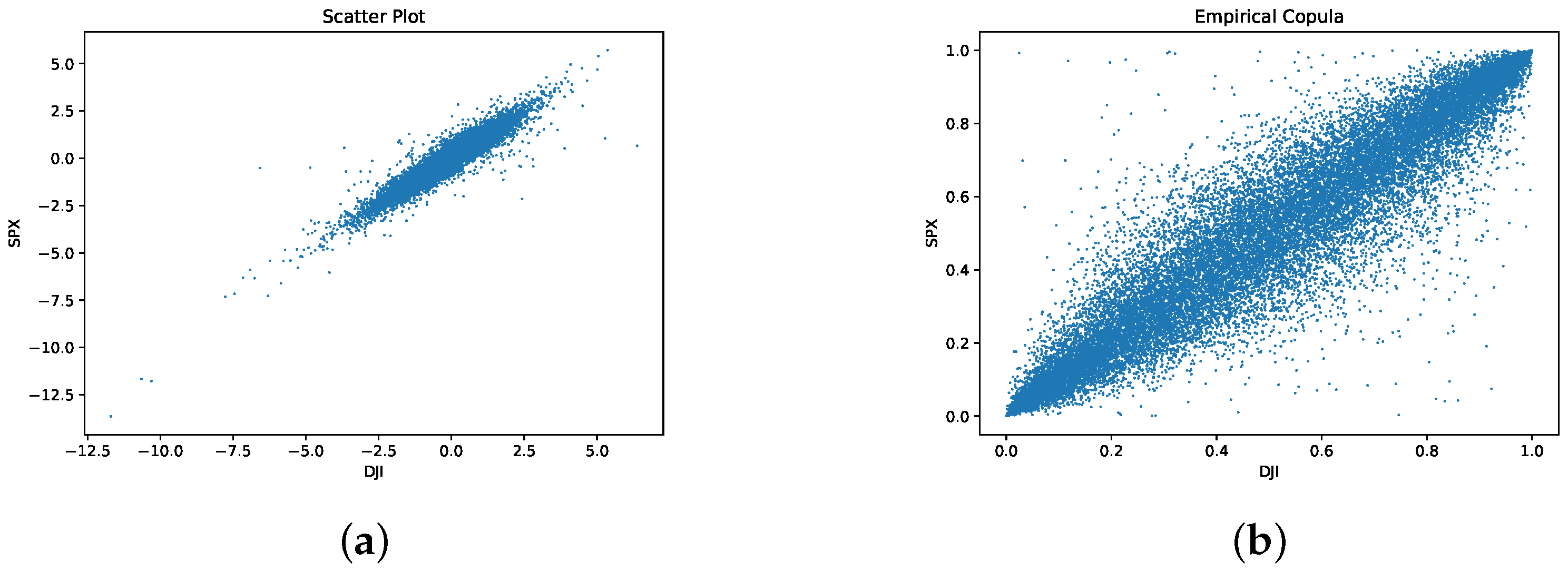
The scatter plot and the empirical copula plot of SPX-DJI innovation pairs estimated by kernel density are presented in Figure 1. The SPX and DJI are strongly correlated especially in the lower and upper tails. Therefore, a powerful copula must reflect the dependence structure of both tails.
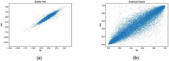
Figure 1.
(a) Scatter plot and (b) empirical copula plot for SPX-DJI innovation pairs.
7. Results
Backtesting is a widely used out-of-sample test, while a goodness of fit test is an in-sample test. We show in this section that NTS innovations and NTS copula perform better than traditional ones on both types of tests.
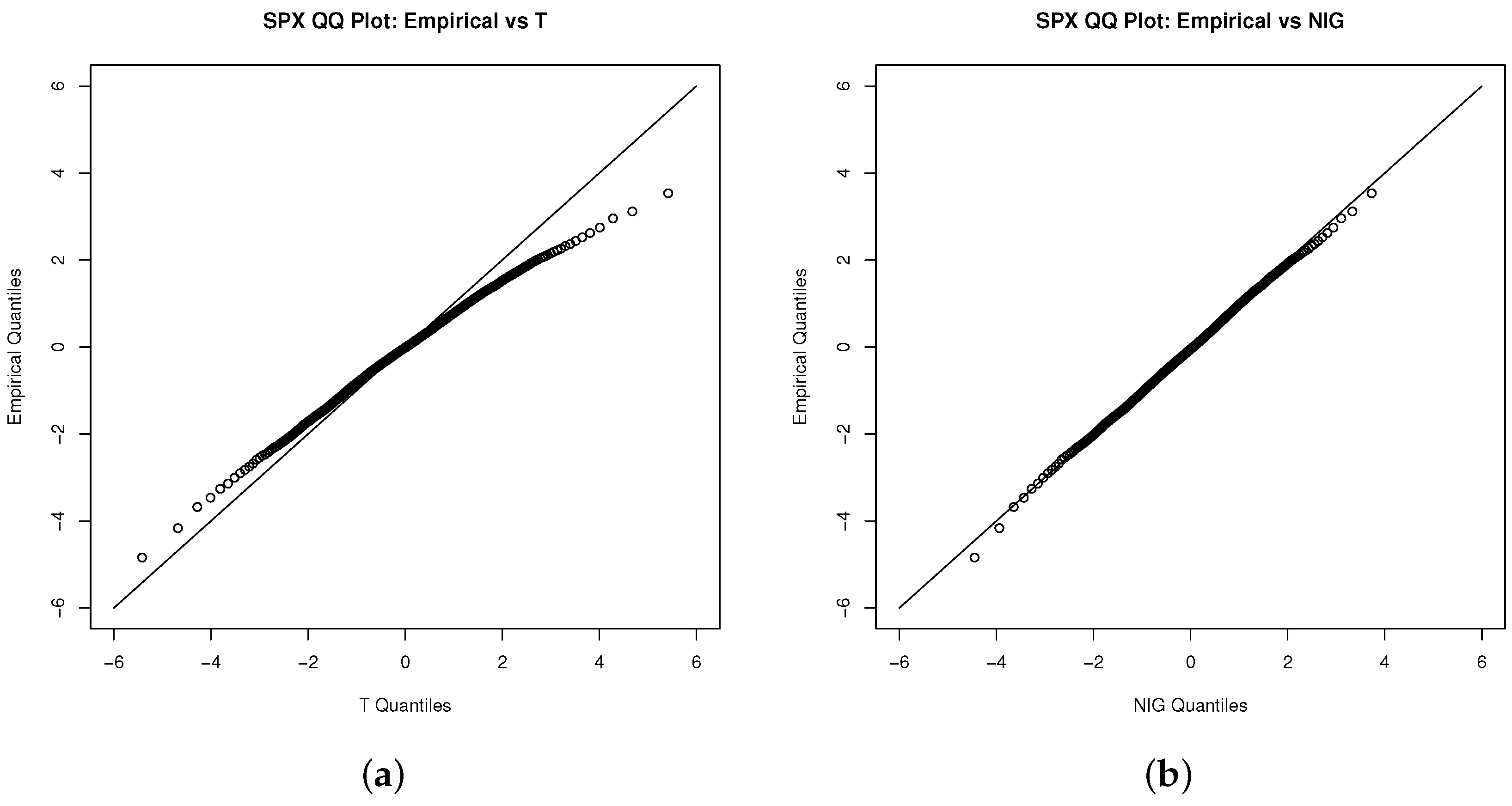
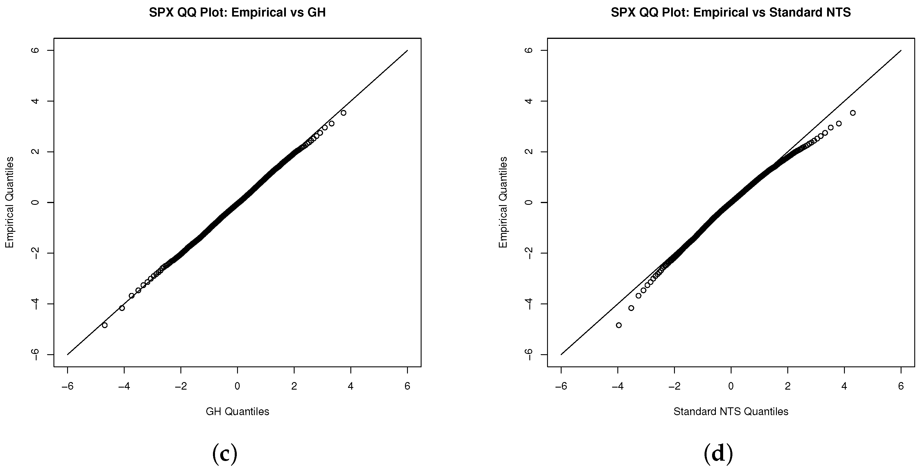
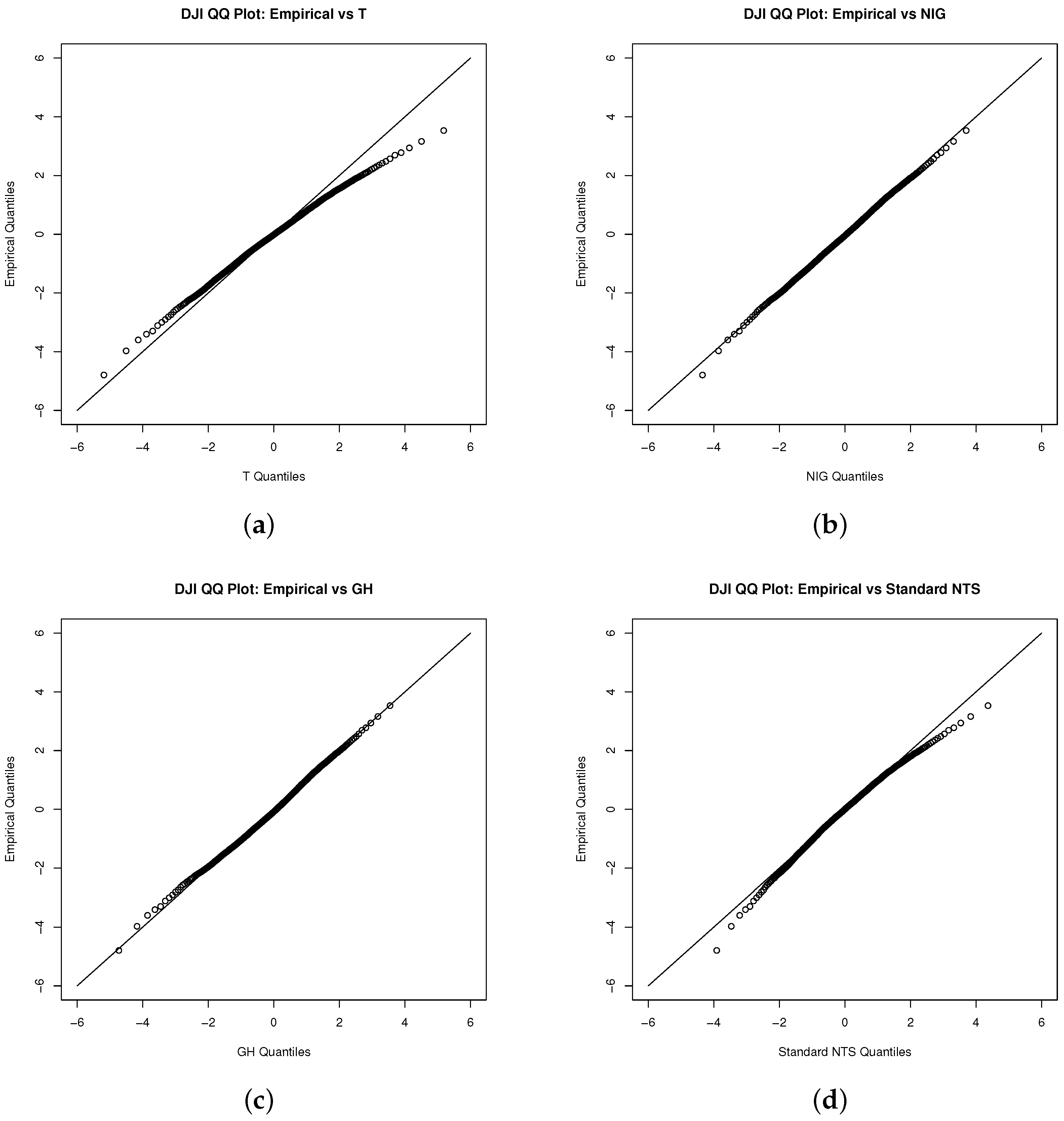
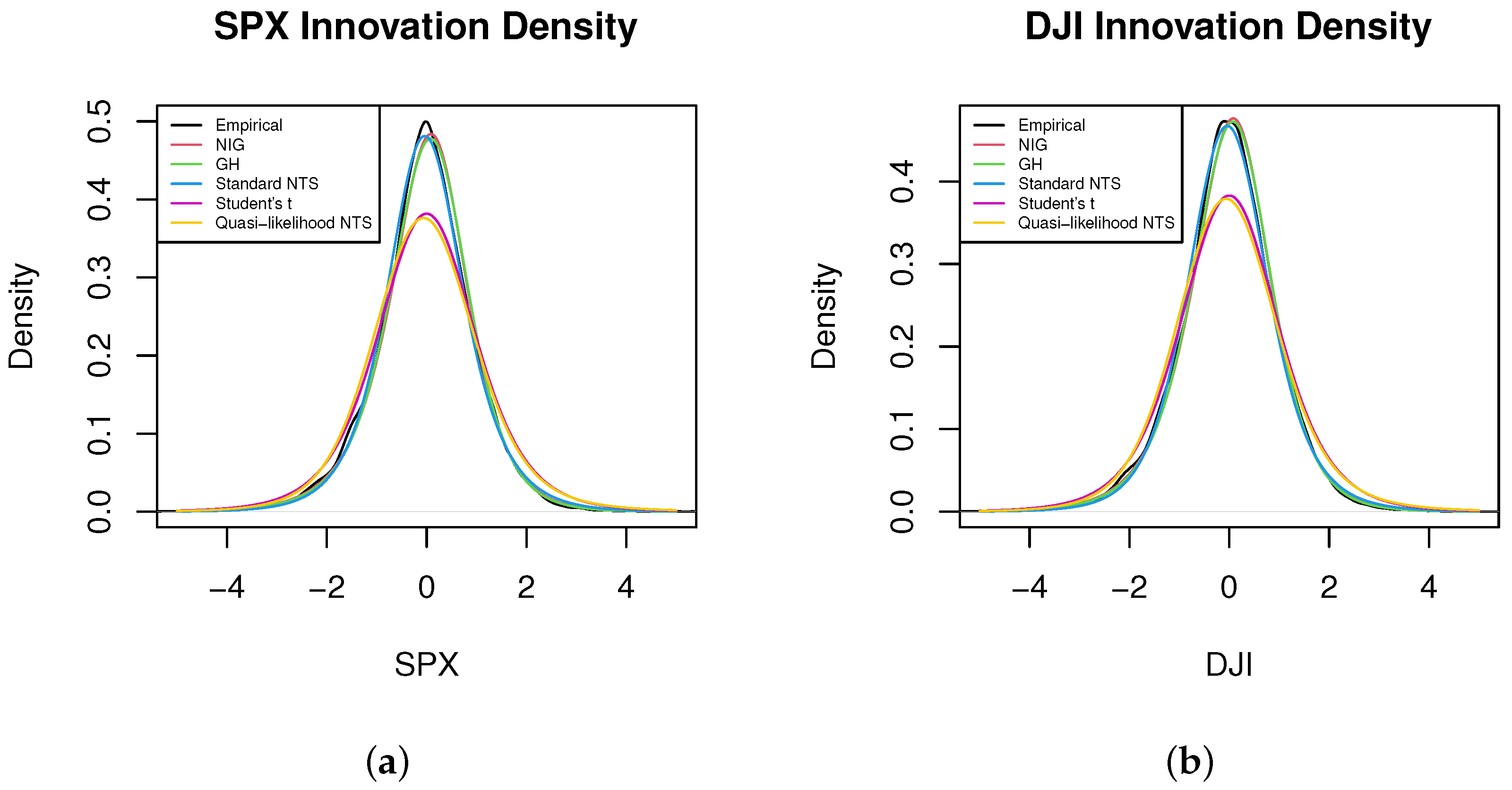
We estimate the standard NTS marginal process via the fitted unconditional Student’s t distribution first. We also demonstrate Student’s t, NIG, and general hyperbolic (GH) distributions as benchmarks. Figure 2, Figure 3 and Figure 6 show that the NIG, GH, and standard NTS fit the marginal density very closely to the empirical density and much better than the Student’s t distribution.


Figure 2.
QQ plot for the innovations of the S&P 500 index with (a) the Student’s t, (b) NIG, (c) GH, and (d) standard NTS distribution.
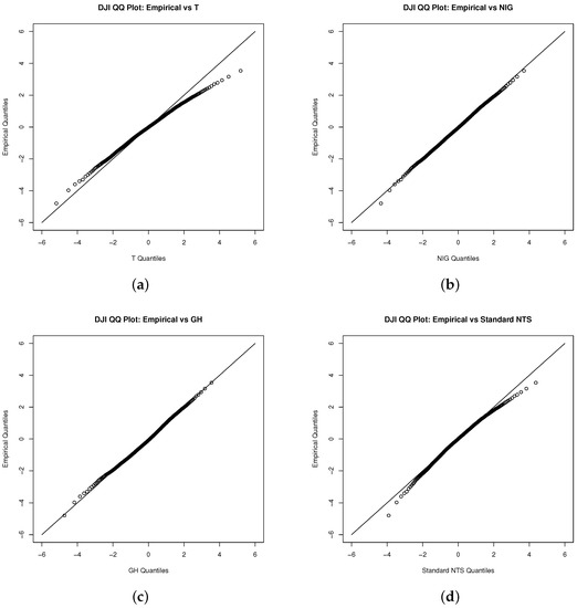
Figure 3.
QQ plot for the innovations of Dow Jones index with (a) the Student’s t, (b) NIG, (c) GH, and (d) standard NTS distribution.
We implement the procedures from Section 4.1 to test our applied quasi-likelihood-based method. The QQ-plots (Figure 4 and Figure 5) of Student’s t and NTS share the same pattern, and are overlapped in density plot (Figure 6). They both reveal that the NTS is indistinguishable from the Student’s t fitting of the innovations.
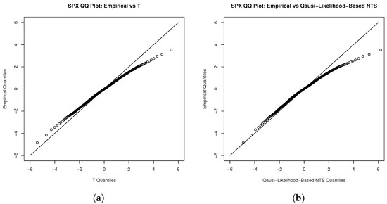
Figure 4.
QQ plot for the innovations of the S&P 500 index with (a) the Student’s t and (b) NTS distribution.
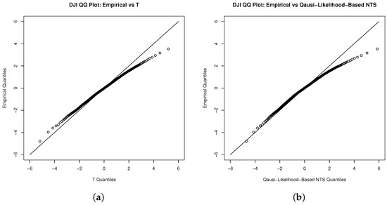
Figure 5.
QQ plot for the innovations of Dow Jones index with (a) Student’s t and (b) NTS distribution.
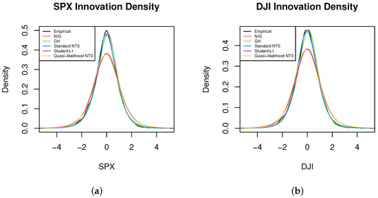
Figure 6.
Density plot for the innovations of the (a) S&P 500 index and (b) Dow Jones index. Magnify figures easier to read.
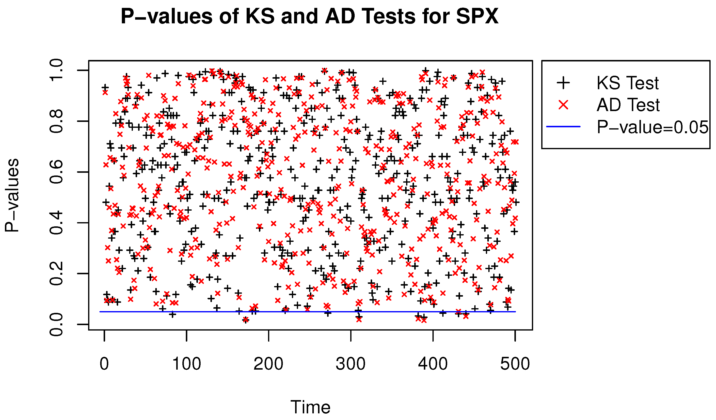
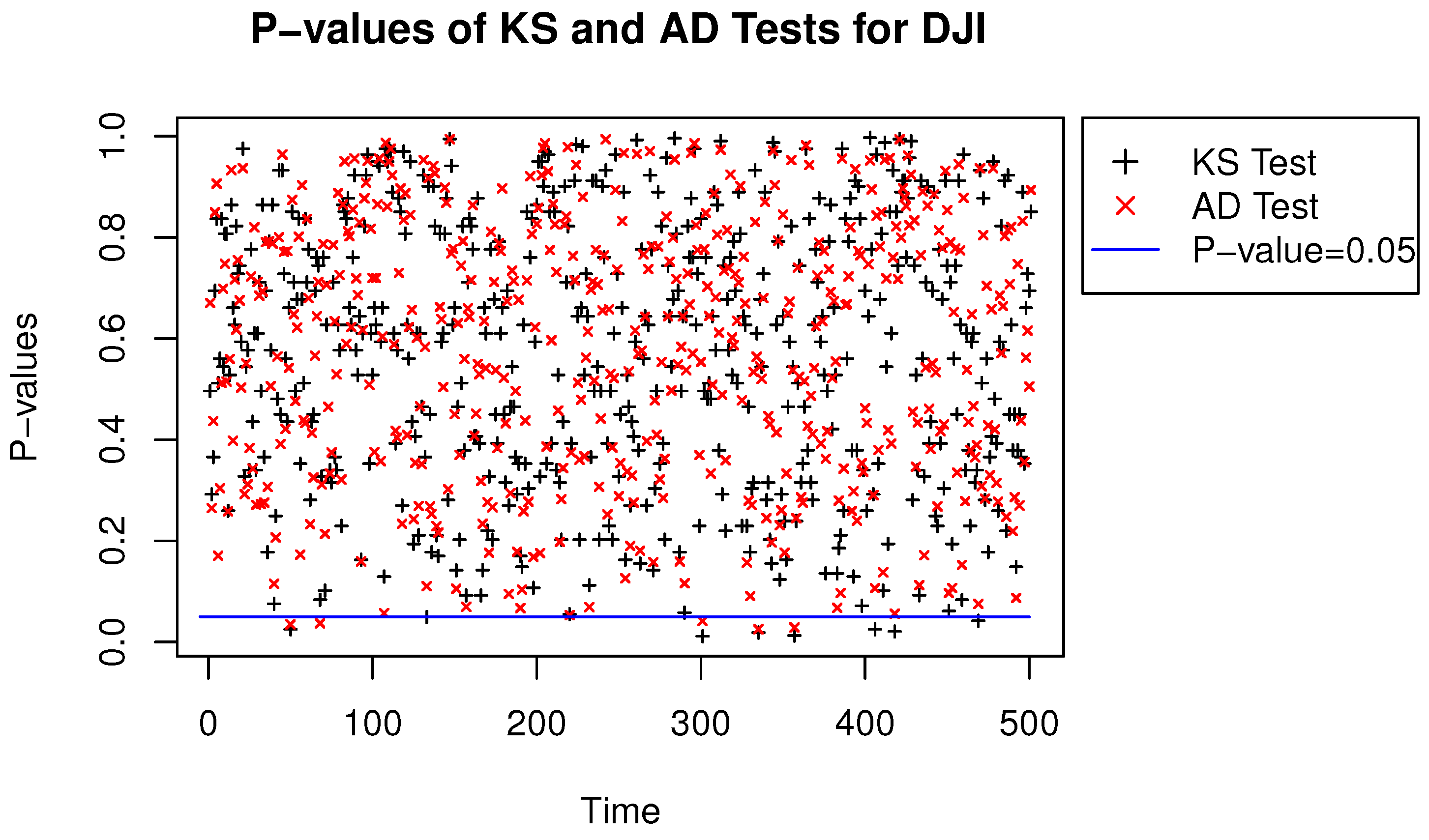
We performed two-sample KS and AD tests for the Student’s t and quasi-likelihood-based NTS distributions, where the SPX and DJI data were both from 3 January 2000 to 9 December 2009 with 2500 samples for each time series. Then we repeated the tests 500 times with one-day-ahead rolling window keeping the width of 2500 samples. The p-values of the two-sample KS and AD statistics with window rolling are shown in Figure 7 and Figure 8. The Figures imply that NTS and the Student’s t distributions are quite indistinguishable. Therefore, the efficient algorithm for estimating NTS innovations is feasible and consistent.
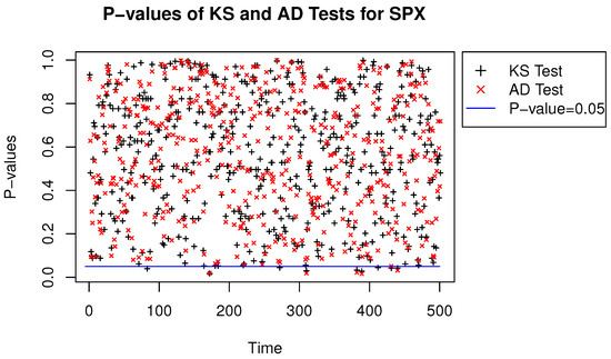
Figure 7.
P-values of the KS and the AD statistics for the S&P 500 index.

Figure 8.
P-values of the KS and AD statistics for the Dow Jones index.
7.1. Test for Copulas
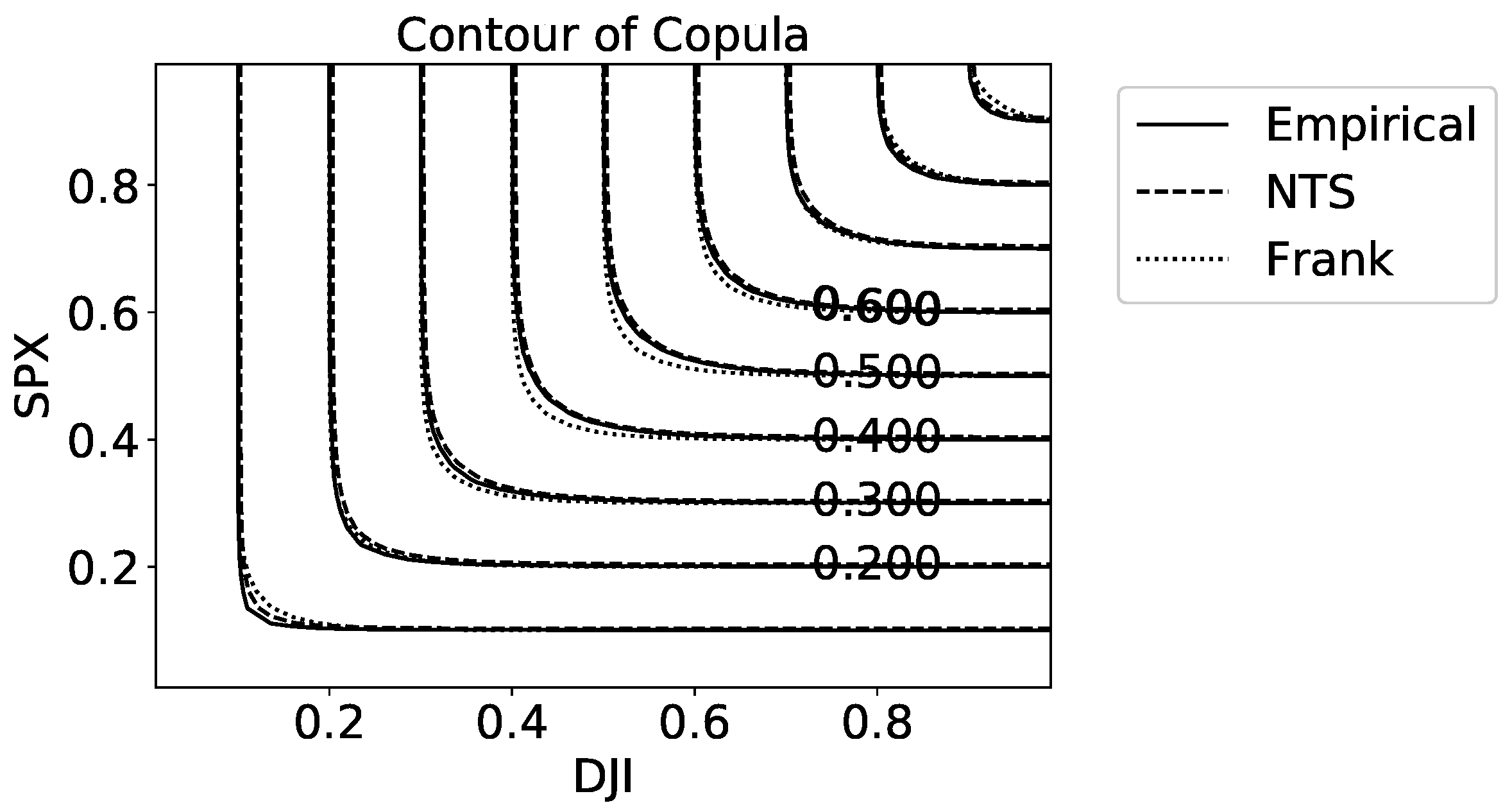
Figure 9 illustrates the density for the empirical copula and the two-dimensional NTS copula. The x-y axis represents the CDF of marginal distributions from 0 to 1, and the z-coordinate shows the estimated copula density . The NTS copula density captures both the upper and lower tail dependence precisely, which means NTS coupla reflects the tail behavior of empirical coupla and hence empirical joint distribution. However, the Archimedean copulas can only capture at most one tail dependence because of their properties. Table 2 supports the point that the NTS copula is superior to the Archimedean copula benchmarks, because the KS statistic of the NTS copula is the lowest. The contour plot (Figure 10) of the copula also suggests that our NTS copula fits the empirical copula much better than the Frank copula, which is the best copula among Archimedean copula benchmarks according to Table 2.
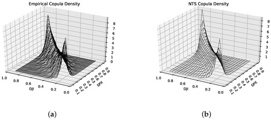
Figure 9.
Density of (a) the empirical copula and (b) the NTS copula.

Table 2.
Two-dimensional test statistics.

Figure 10.
Contour plot of the copula estimated by different copulas.
7.2. Backtesting
We applied the rolling/sliding window approach to do the backtesting with a window width equal to 500 days. After estimating all the parameters and CoVaR on day t, the window moved forward by one day, with the window width remaining unchanged.
Table 3 gives the backtesting results from the modified Kupiec’s test corrected by the joint distribution. There were 23,943 samples in total for backtesting, and the expected numbers of exceedances are listed in the last column as a benchmark. According to Table 2, the Frank copula is still the best copula in the Archimedean copula family in light of the number of exceedances. However, the Lévy-Clayton copula produces results far closer to the expected number than the Archimedean copula family, which means it has good performance in the tail. The NTS copula has a similar performance to the Lévy-Clayton copula but with a much more accurate fit to the global empirical copula.

Table 3.
The actual and expected number of exceedances from backtesting.
7.3. CoVaR and CoVaR
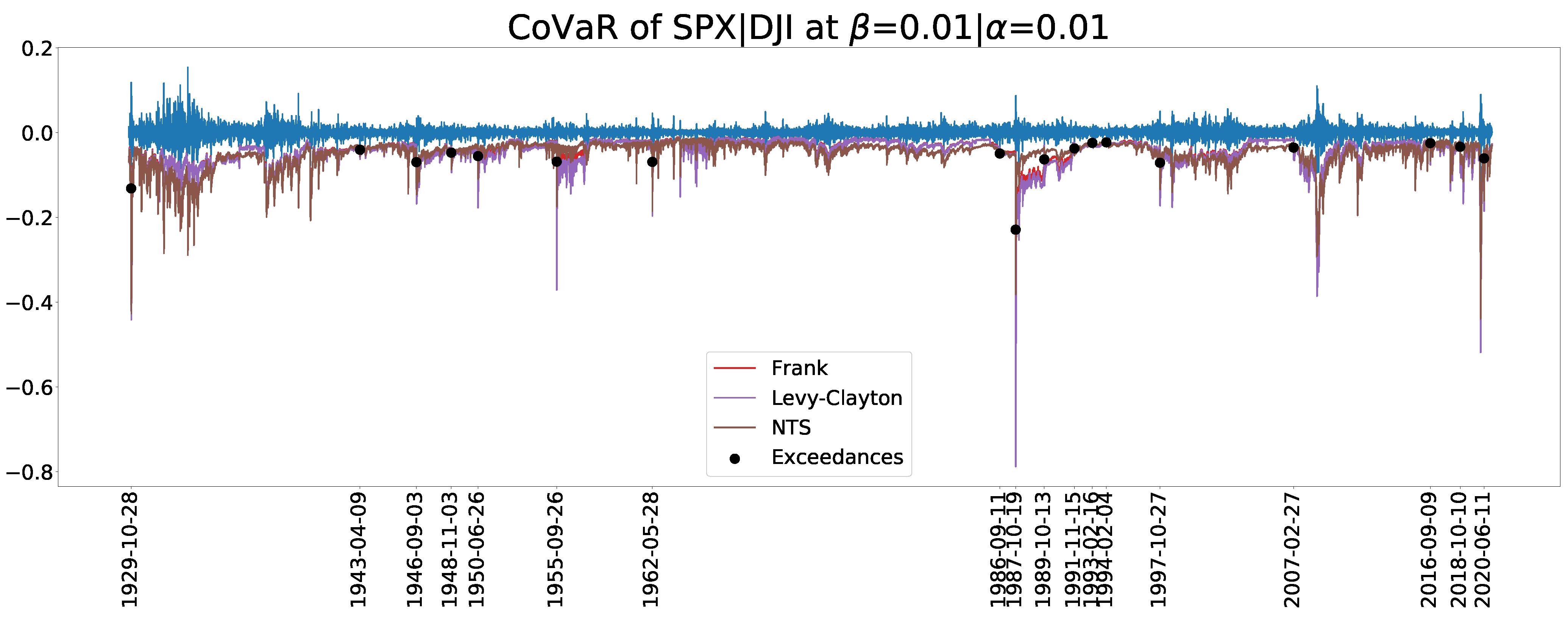
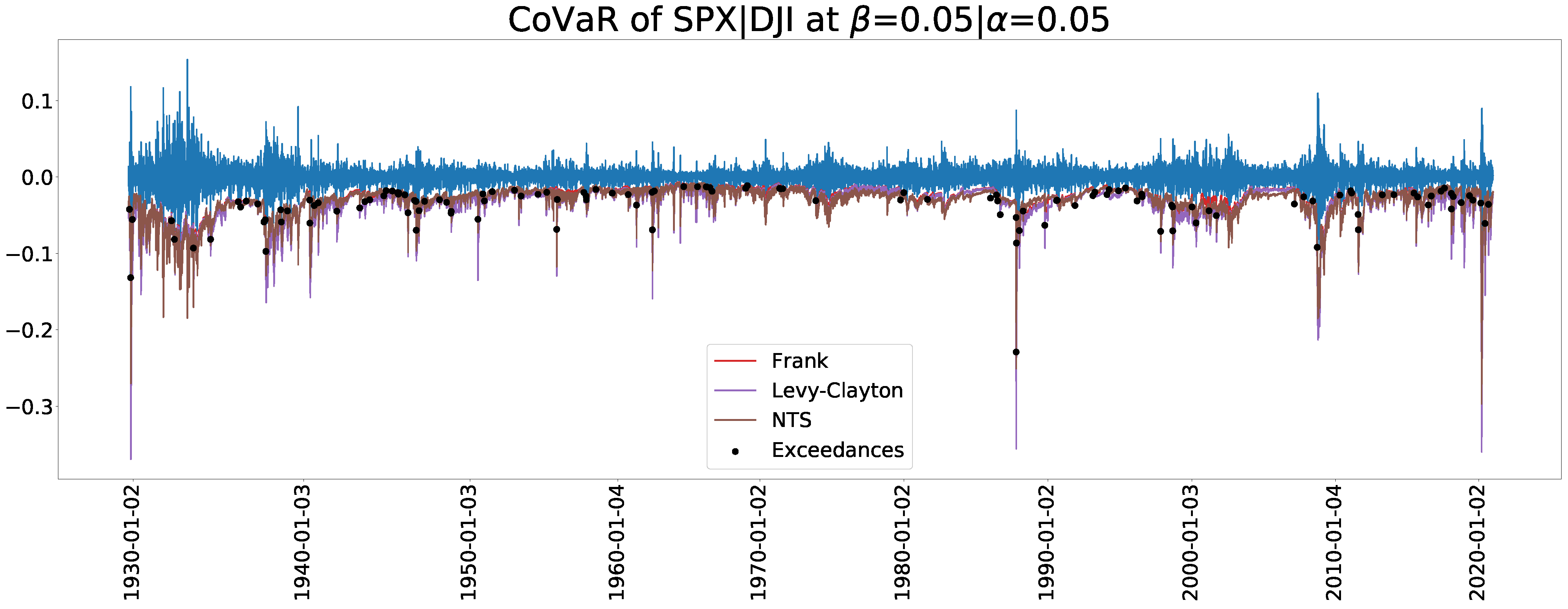
Figure 11 and Figure 12 display the estimated CoVaR when and , respectively. In particular, Figure 11 depicts the date when the exceedances of CoVaR derived from the NTS copula occurred. To make the Figure distinguishable and clearer, we only show the results of the Frank copula as a representative of the Archimedean copula family because it has the best in-sample test performance except for the NTS. The estimated CoVaRs of the Archimedean copula family is far higher than those of the NTS copula.
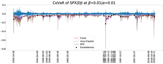
Figure 11.
A CoVaR plot for .
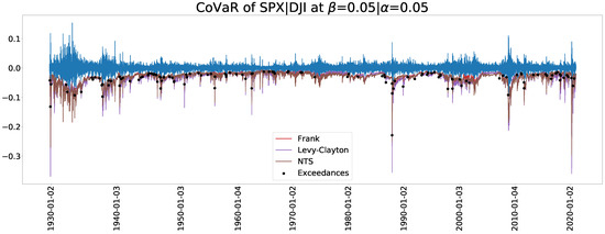
Figure 12.
A CoVaR plot for .
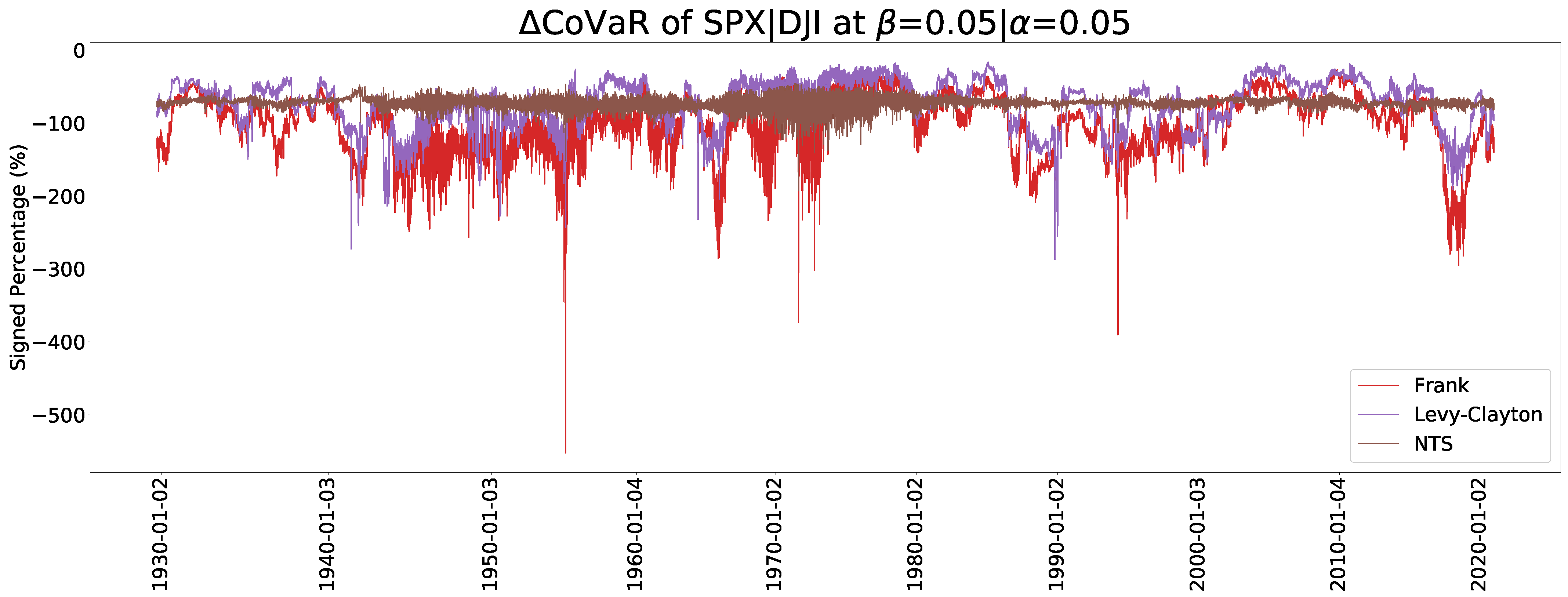
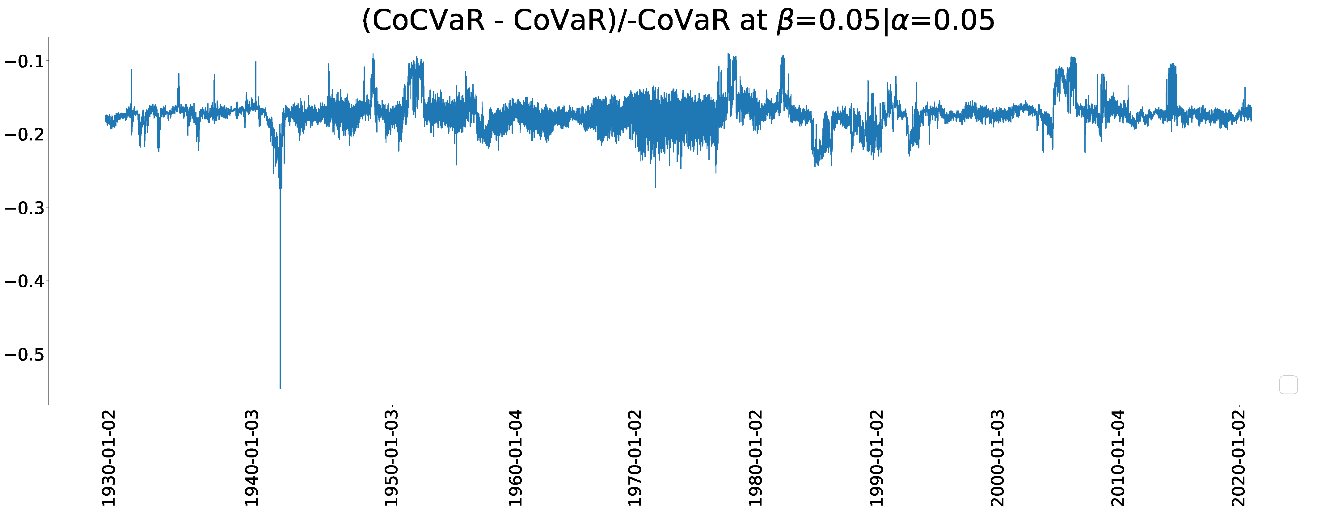
Figure 13 and Figure 14 show the estimated CoVaR when and , respectively. The Archimedean copula family has a dramatic change of CoVaR whereas the NTS copula is more stable. The stable values of change can be comparable with previous crisis and provide more information. We can also use the relative difference between CoCVaR and CoVaR for the early warning of crisis, where the relative difference (RD) is defined by
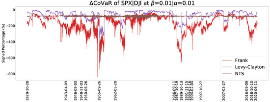
Figure 13.
A CoVaR plot for .

Figure 14.
A CoVaR plot for .
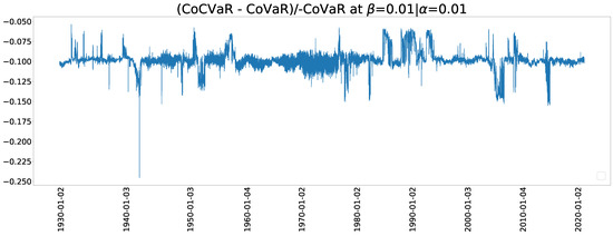
Figure 15.
A relative difference between CoCVaR and CoVaR plot for .
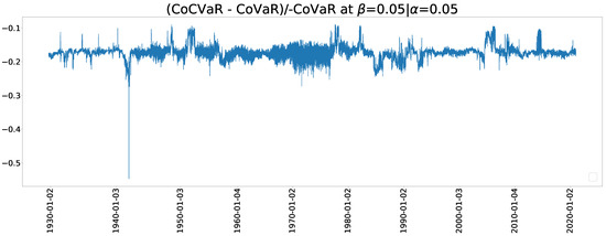
Figure 16.
A relative difference between CoCVaR and CoVaR for .
8. Conclusions
We applied the NTS copula, which belongs to the Lévy copula family, for modeling CoVaR. Our results obtained from extensive backtesting and goodness of fit testing show that the NTS copula models the dependence structure more accurately than traditional copulas. We also proposed a modified Kupiec’s test that accounts for the uncertainty of the estimated VaR. This translates to a test that is more stable when the data sizes are not of sufficient lengths.
Author Contributions
Conceptualization, S.T.R. and J.G.; methodology, Y.S.K.; software, Y.S.K. and Y.L.; validation, Y.S.K. and Y.L.; formal analysis, Y.S.K. and S.T.R.; investigation, Y.L.; resources, Y.L.; data curation, Y.L.; writing—original draft preparation, Y.L.; writing—review and editing, P.M.D. and A.S.K.; visualization, Y.L.; supervision, P.M.D., S.T.R. and J.G.; project administration, J.G.; funding acquisition, J.G. All authors have read and agreed to the published version of the manuscript.
Funding
This research received no external funding.
Data Availability Statement
Publicly available datasets were analyzed in this study. This data can be found here: [https://stooq.pl/].
Acknowledgments
In this section, you can acknowledge any support given which is not covered by the author contribution or funding sections. This may include administrative and technical support, or donations in kind (e.g., materials used for experiments).
Conflicts of Interest
The authors declare no conflict of interest.
Note
| 1. | https://rdrr.io/github/aaron9011/temStaR-v0.814/ (accessed on 4 June 2021) |
References
- Acharya, Viral V., Lasse H. Pedersen, Thomas Philippon, and Matthew Richardson. 2017. Measuring systemic risk. The Review of Financial Studies 30: 2–47. [Google Scholar] [CrossRef]
- Acharya, Viral V., Hyun Song Shin, and Tanju Yorulmazer. 2011. Crisis resolution and bank liquidity. The Review of Financial Studies 24: 2166–205. [Google Scholar] [CrossRef]
- Adrian, Tobias, and Markus K. Brunnermeier. 2011. CoVaR. Technical Report. Cambridge: National Bureau of Economic Research. [Google Scholar]
- Allen, Linda, Turan G. Bali, and Yi Tang. 2012. Does systemic risk in the financial sector predict future economic downturns? The Review of Financial Studies 25: 3000–36. [Google Scholar] [CrossRef]
- Anand, Abhinav, Tiantian Li, Tetsuo Kurosaki, and Young Shin Kim. 2016. Foster–hart optimal portfolios. Journal of Banking & Finance 68: 117–30. [Google Scholar]
- Barndorff-Nielsen, Ole E. 1997. Normal inverse gaussian distributions and stochastic volatility modelling. Scandinavian Journal of Statistics 24: 1–13. [Google Scholar] [CrossRef]
- Barndorff-Nielsen, Ole Eiler, and Sergei Z. Levendorskii. 2001. Feller processes of normal inverse gaussian type. Quantitative Finance 1: 318–31. [Google Scholar] [CrossRef]
- Barndorff-Nielsen, Ole E., and Neil Shephard. 2001. Normal Modified Stable Processes. Oxford: Citeseer. [Google Scholar]
- Basel Committee on Banking Supervision. 2009. Principles for Sound Stress Testing Practices and Supervision. Available online: https://www.bis.org/publ/bcbs155.htm (accessed on 4 June 2021).
- Bernardi, Mauro, Fabrizio Durante, and Piotr Jaworski. 2017. Covar of families of copulas. Statistics & Probability Letters 120: 8–17. [Google Scholar]
- Bianchi, Michele Leonardo, and Alberto Maria Sorrentino. 2020. Measuring covar: An empirical comparison. Computational Economics 55: 511–28. [Google Scholar] [CrossRef]
- Braiek, Sana, Rihab Bedoui, and Lotfi Belkacem. 2020. Islamic portfolio optimization under systemic risk: Vine copula-covar based model. International Journal of Finance & Economics. [Google Scholar] [CrossRef]
- Brownlees, Christian, and Robert F. Engle. 2017. Srisk: A conditional capital shortfall measure of systemic risk. The Review of Financial Studies 30: 48–79. [Google Scholar] [CrossRef]
- Cerutti, Eugenio, Stijn Claessens, and Patrick McGuire. 2012. Systemic Risks in Global Banking: What Available Data Can Tell Us and What More Data Are Needed? Technical Report. Cambridge: National Bureau of Economic Research. [Google Scholar]
- Chollete, Lorán, Andréas Heinen, and Alfonso Valdesogo. 2009. Modeling international financial returns with a multivariate regime-switching copula. Journal of Financial Econometrics 7: 437–80. [Google Scholar] [CrossRef]
- Cohen, Joel E., Richard A. Davis, and Gennady Samorodnitsky. 2020. Heavy-tailed distributions, correlations, kurtosis and taylor’s law of fluctuation scaling. Proceedings of the Royal Society A 476: 20200610. [Google Scholar] [CrossRef] [PubMed]
- Danielsson, Jon, Bjørn N. Jorgensen, Sarma Mandira, Gennady Samorodnitsky, and Casper G. De Vries. 2005. Subadditivity Re-Examined: The Case for Value-at-Risk. Technical Report. Ithaca: Cornell University, Operations Research and Industrial Engineering. [Google Scholar]
- De Luca, Giovanni, and Giorgia Rivieccio. 2012. Multivariate tail dependence coefficients for archimedean copulae. In Advanced Statistical Methods for the Analysis of Large Data-Sets. Berlin and Heidelberg: Springer, pp. 287–96. [Google Scholar]
- Delbaen, Freddy, and Walter Schachermayer. 1999. The Fundamental Theorem of Asset Pricing for Unbounded Stochastic Processes. Vienna: SFB Adaptive Information Systems and Modelling in Economics and Management. [Google Scholar]
- Di Bernardino, Elena, Véronique Maume-Deschamps, and Clémentine Prieur. 2013. Estimating a bivariate tail: A copula based approach. Journal of Multivariate Analysis 119: 81–100. [Google Scholar] [CrossRef]
- Du, Zaichao, and Juan Carlos Escanciano. 2017. Backtesting expected shortfall: Accounting for tail risk. Management Science 63: 940–58. [Google Scholar] [CrossRef]
- Eberlein, Ernst, and Dilip B. Madan. 2009. On correlating Lévy processes. Robert H. Smith School Research Paper No. RHS, 6–118. [Google Scholar] [CrossRef]
- Eberlein, Ernst, and Fehmi Özkan. 2005. The lévy libor model. Finance and Stochastics 9: 327–48. [Google Scholar] [CrossRef]
- Embrechts, Paul, Hansjorg Furrer, and Roger Kaufmann. 2003. Quantifying regulatory capital for operational risk. Derivatives Use, Trading and Regulation 9: 217–33. [Google Scholar]
- Emmer, Susanne, Marie Kratz, and Dirk Tasche. 2015. What is the best risk measure in practice? A comparison of standard measures. Journal of Risk 18: 2. [Google Scholar] [CrossRef]
- Forbes, Kristin, and Roberto Rigobon. 2001. Measuring contagion: Conceptual and empirical issues. In International Financial Contagion. Berlin and Heidelberg: Springer, pp. 43–66. [Google Scholar]
- Frahm, Gabriel. 2004. Generalized Elliptical Distributions: Theory and Applications. Ph.D. Thesis, Universität zu Köln, Köln, Germany. [Google Scholar]
- Garcia, René, Eric Renault, and David Veredas. 2011. Estimation of stable distributions by indirect inference. Journal of Econometrics 161: 325–37. [Google Scholar] [CrossRef]
- Garcia, René, and Georges Tsafack. 2008. Dependence Structure and Extreme Comovements in International Equity and Bond Markets with Portfolio Diversification Effects. Working Paper. Risk Asset Management Research Centre: Available online: http://dx.doi.org/10.2139/ssrn.1107718 (accessed on 4 June 2021).
- Giglio, Stefano, Bryan Kelly, and Seth Pruitt. 2016. Systemic risk and the macroeconomy: An empirical evaluation. Journal of Financial Economics 119: 457–71. [Google Scholar] [CrossRef]
- Girardi, Giulio, and A. Tolga Ergün. 2013. Systemic risk measurement: Multivariate garch estimation of covar. Journal of Banking & Finance 37: 3169–80. [Google Scholar]
- Härdle, Wolfgang K., Ostap Okhrin, and Weining Wang. 2012. HMM in Dynamic HAC Models. Available online: http://dx.doi.org/10.2139/ssrn.2894223 (accessed on 4 June 2021).
- Heffernan, Janet E. 2000. A directory of coefficients of tail dependence. Extremes 3: 279–90. [Google Scholar] [CrossRef]
- Huang, Wei-Qiang, and Stanislav P. Uryasev. 2018. The cocvar approach: Systemic risk contribution measurement. Journal of Risk 20: 4. [Google Scholar] [CrossRef]
- Jaworski, Piotr. 2017. On conditional value at risk (covar) for tail-dependent copulas. Dependence Modeling 5: 1–19. [Google Scholar] [CrossRef]
- Jaworski, Piotr, Fabrizio Durante, Wolfgang Karl Hardle, and Tomasz Rychlik. 2010. Copula Theory and Its Applications. Berlin and Heidelberg: Springer, vol. 198. [Google Scholar]
- Kanas, Angelos, and Panagiotis D. Zervopoulos. 2020. Systemic risk-shifting in us commercial banking. Review of Quantitative Finance and Accounting 54: 517–39. [Google Scholar] [CrossRef]
- Karimalis, Emmanouil N., and Nikos K. Nomikos. 2018. Measuring systemic risk in the european banking sector: A copula covar approach. The European Journal of Finance 24: 944–75. [Google Scholar] [CrossRef]
- Kim, Young Shin, Svetlozar T. Rachev, Michele Leonardo Bianchi, Ivan Mitov, and Frank J. Fabozzi. 2011. Time series analysis for financial market meltdowns. Journal of Banking & Finance 35: 1879–91. [Google Scholar]
- Kim, Young Shin, and David S. Volkmann. 2013. Normal tempered stable copula. Applied Mathematics Letters 26: 676–80. [Google Scholar] [CrossRef]
- Kritzman, Mark, Yuanzhen Li, Sebastien Page, and Roberto Rigobon. 2011. Principal components as a measure of systemic risk. The Journal of Portfolio Management 37: 112–26. [Google Scholar] [CrossRef]
- Liebscher, Eckhard. 2008. Construction of asymmetric multivariate copulas. Journal of Multivariate analysis 99: 2234–50. [Google Scholar] [CrossRef]
- Lien, Donald, Gerui Lim, Li Yang, and Chunyang Zhou. 2013. Dynamic dependence between liquidity and the s&p 500 index futures-cash basis. Journal of Futures Markets 33: 327–42. [Google Scholar]
- Lin, Edward M. H., Edward W. Sun, and Min-Teh Yu. 2018. Systemic risk, financial markets, and performance of financial institutions. Annals of Operations Research 262: 579–603. [Google Scholar] [CrossRef]
- Low, Rand Kwong Yew, Jamie Alcock, Robert Faff, and Timothy Brailsford. 2013. Canonical vine copulas in the context of modern portfolio management: Are they worth it? Journal of Banking & Finance 37: 3085–99. [Google Scholar]
- Low, Rand Kwong Yew, Robert Faff, and Kjersti Aas. 2016. Enhancing mean–variance portfolio selection by modeling distributional asymmetries. Journal of Economics and Business 85: 49–72. [Google Scholar] [CrossRef]
- Mainik, Georg, and Eric Schaanning. 2014. On dependence consistency of CoVaR and some other systemic risk measures. Statistics & Risk Modeling 31: 49–77. [Google Scholar]
- Nguyen, Tilo, and Gennady Samorodnitsky. 2013. Multivariate tail estimation with application to analysis of covar. Astin Bulletin 43: 245–70. [Google Scholar] [CrossRef]
- Pourkhanali, Armin, Jong-Min Kim, Laleh Tafakori, and Farzad Alavi Fard. 2016. Measuring systemic risk using vine-copula. Economic Modelling 53: 63–74. [Google Scholar] [CrossRef]
- Pritsker, Matt. 2001. The channels for financial contagion. In International Financial Contagion. Berlin and Heidelberg: Springer. [Google Scholar]
- Reboredo, Juan C., and Andrea Ugolini. 2015. Systemic risk in european sovereign debt markets: A covar-copula approach. Journal of International Money and Finance 51: 214–44. [Google Scholar] [CrossRef]
- Rémillard, Bruno, Nicolas Papageorgiou, and Frédéric Soustra. 2012. Copula-based semiparametric models for multivariate time series. Journal of Multivariate Analysis 110: 30–42. [Google Scholar] [CrossRef]
- Rivera-Castro, Miguel A., Andrea Ugolini, and Juan Arismendi Zambrano. 2018. Tail systemic risk and contagion: Evidence from the brazilian and latin america banking network. Emerging Markets Review 35: 164–89. [Google Scholar] [CrossRef]
- Sato, Ken-Iti. 1999. Lévy Processes and Infinitely Divisible Distributions. Cambridge: Cambridge University Press. [Google Scholar]
- Schoutens, Wim. 2003. Lévy Processes in Finance: Pricing Financial Derivatives. Leuven: KU LEUVEN. [Google Scholar] [CrossRef]
- Segoviano Basurto, Miguel, and Charles Goodhart. 2009. Banking Stability Measures. IMF Working Paper. Washington: International Monetary Fund, pp. 1–54. [Google Scholar]
- Shiryaev, Albert N. 1999. Essentials of Stochastic Finance: Facts, Models, Theory. Singapore: World Scientific, vol. 3. [Google Scholar]
- Sklar, M. 1959. Fonctions de repartition an dimensions et leurs marges. Publications de L Institut de Statistique de L Universite de Paris. 8: 229–31. [Google Scholar]
- Smaga, Pawel. 2014. The Concept of Systemic Risk. London: Systemic Risk Centre, London School of Economics and Political Science. [Google Scholar]
- Tankov, Peter. 2016. Lévy copulas: Review of recent results. In The Fascination of Probability, Statistics and Their Applications. Edited by Mark Podolskij, Robert Stelzer, Steen Thorbjørnsen and Almut E. D. Veraart. Cham: Springer, pp. 127–51. [Google Scholar]
- Targino, Rodrigo S., Gareth W. Peters, and Pavel V. Shevchenko. 2015. Sequential Monte Carlo samplers for capital allocation under copula-dependent risk models. Insurance: Mathematics and Economics 61: 206–26. [Google Scholar] [CrossRef]
- Tobias, Adrian, and Markus K. Brunnermeier. 2016. CoVaR. The American Economic Review 106: 1705. [Google Scholar]
- Yang, Lu, Jason Z. Ma, and Shigeyuki Hamori. 2018. Dependence structures and systemic risk of government securities markets in central and eastern europe: A covar-copula approach. Sustainability 10: 324. [Google Scholar] [CrossRef]
- Zhang, Jianlin. 2015. Systemic Risk Measure: CoVaR and Copula. Master’s Thesis, Humboldt University at Berlin, Berlin. [Google Scholar]
- Zhang, Jin, and Dietmar Maringer. 2010. Asset Pair-Copula Selection with Downside Risk Minimization. Technical Report. Available online: https://ideas.repec.org/p/com/wpaper/037.html (accessed on 4 June 2021).
Publisher’s Note: MDPI stays neutral with regard to jurisdictional claims in published maps and institutional affiliations. |
© 2021 by the authors. Licensee MDPI, Basel, Switzerland. This article is an open access article distributed under the terms and conditions of the Creative Commons Attribution (CC BY) license (https://creativecommons.org/licenses/by/4.0/).

