Abstract
This paper proposes a conceptual modeling framework based on category theory that serves as a tool to study common structures underlying diverse approaches to modeling credit default that at first sight may appear to have nothing in common. The framework forms the basis for an entropy-based stacking model to address issues of inconsistency and bias in classification performance. Based on the Lending Club’s peer-to-peer loans dataset and Taiwanese credit card clients dataset, relative to individual base models, the proposed entropy-based stacking model provides more consistent performance across multiple data environments and less biased performance in terms of default classification. The process itself is agnostic to the base models selected and its performance superior, regardless of the models selected.
1. Introduction
Credit risk assessment is a critical component of a lender’s loan approval, monitoring and pricing process. It is achieved through the application of statistical models that provide estimates of the probability of default (PD) of the borrower, usually over a one-year period. Default risk is typically treated as a dichotomous classification problem, distinguishing potential defaulters (payers) from non-defaulters (non-payers) with information about default status contained within a set of features of the parties involved in the transaction. Altman (1968) provided the first formal approach towards corporate default modeling, reconciling accounting-based ratios often used by practitioners with rigorous statistical techniques championed by researchers. He applies a statistical technique called Multivariate Discriminant Analysis (MDA) to construct discriminant functions (axes) from linear combinations of the selected covariates. A major drawback of MDA is the large number of unrealistic assumptions imposed, which frequently results in biased significance tests and error rates (Joy and Tollefson 1978; Mcleay and Omar 2000). This has led many researchers to propose logistic models as the next best alternative, requiring fewer restrictive assumptions and allowing for more general usage without loss in performance (Altman and Sabato 2007; Lawrence et al. 1992; Martin 1977; Ohlson 1980).
Whilst there have been several attempts to put the field of credit risk modeling on a more concrete theoretical foundation (Asquith et al. 1989; Jonkhart 1979; Santomero and Vinso 1977; Vassalou and Xing 2004), supported by advances in computing power, the literature has more recently moved to techniques employed in the field of machine learning (ML). Essentially, it consists of statistical models that require less restrictive assumptions regarding the data, providing more flexibility in model construction and usage. It has made this approach the fastest growing research area in credit risk modeling. Among supervised machine learning methods, Artificial Neural Network (ANN) has received most attention, offering improved prediction accuracy, adaptive capability and robustness (Dastile et al. 2020; Tam 1991).
Since its inception, the number of studies using ML techniques has increased nearly exponentially, focusing primarily on benchmarking state of the art individual classifiers. Lessmann et al. (2015) is the first study to benchmark a wide range of supervised ML classifiers not investigated previously. It has become a key reference for other researchers on model comparison. Also notable is the study of Teply and Polena (2020), applying ML to peer-to-peer loan dataset provided by the Lending Club. Of particular interest has been the construction of ensembles of credit risk models (Abellán and Mantas 2014; Ala’raj and Abbod 2016b; Finlay 2011; Hsieh and Hung 2010) and meta-classifiers trained on combined outputs of groups of base models (Doumpos and Zopounidis 2007; Lessmann et al. 2015; Wang et al. 2018; Wolpert 1992; Xia et al. 2018).
Despite the increasing sophistication in how individual base models are put together in an ensemble (stacking) or how the various outputs are combined to achieve final prediction, all face a critical issue. Essentially, there is a lack of a sound conceptual framework to guide the ensemble or stacking process. Each study specifies their own method of selecting base models for combination and generating combined outputs. As a result, the recommendations made have been highly sensitive to the data environments examined, making it difficult to perform sound comparative performance analysis. This explains why each study tends to conclude that their combination method is the best performer among competing models.
Motivated by a lack of consistency in model selection, this paper outlines a conceptual framework concerned with the design of structures in credit risk modeling within a classification context. Based on the framework, various computational approaches are proposed that solves the above noted problem of inconsistency in results. First, category theory is introduced to help design common structures underlying seemingly unrelated credit risk models. These structures reveal deep connection between seemingly unrelated models, thus providing a powerful tool to study their relationships without being distracted by details of their implementation. Second, a stacking model is constructed to address issues of inconsistent and biased performance in model benchmarking. Typically, a model’s predictive value exhibits inconsistent performance when there are changes in data scope within an environment or changes in the environment itself, with the underlying model essentially remaining unchanged. Complicating this issue is a tendency for models to be biased in their prediction due to the subjective selection of performance criteria. It is not unusual to observe a model delivering an impressive overall performance, while failing to detect any credit default at all. In order to address this issue, two new structures—Shannon’s information entropy and enriched categories—are introduced. The focus of attention is on demonstrating the benefit of having a sound conceptual framework to enable optimal construction of models that minimise performance inconsistency and bias.
The proposed modeling framework is applied to the Lending Club’s peer-to-peer loans dataset from 2007–2013 as well as to Taiwanese credit card clients dataset for 2005. The empirical results show that the proposed entropy-based stacking approach results in more consistent performance across multiple data environments as well as less biased performance. The process itself is agnostic as to which base model is selected. The conceptual framework developed provides an explanation as to why various ensemble and stacking models proposed in the literature arrive at different conclusions regarding classification performance—they are caught in an equivalence trap. Ensemble models, despite their seemingly sophisticated assembling process, fuse the outputs of base models either by majority voting or by some type of linear weighted combination. In doing so, no new instance of data structure is created; all that has been achieved is an extension of the operation to cover the output combination process. As a result, the categorical structure of the modeling approach is the same as that of any other credit risk model with equivalent performance.
This paper is organized as follows. Section 2 describes in detail the modeling framework proposed, including key elements of a category and how the representation of current approaches to modeling credit risk can be built within the context of frames. Section 3 presents the data, whilst Section 4 presents the empirical results. A discussion of the empirical findings is presented in Section 5. Finally, Section 6 concludes the paper.
2. Modeling Framework
2.1. Categorial Equivalence
Whilst at a first glance, the many statistical approaches to credit risk modeling may seem radically different from one another, with each model constructing its own relation between the various covariates, common features exist which can be integrated into a conceptual framework that captures the essence of the credit modeling process. This framework can be built on the concept of category theory, which is the abstract study of process first proposed by Eilenberg and MacLane (1945). Category theory concerns itself with how different modeling approaches relate to one another and the manner in which they relate to one another is related to the functions between them. Instead of focusing on a particular credit risk modeling approach A and asking what its elements are, category theory asks what all the morphisms from A to other modeling approaches. Arguably, this mindset could be extremely useful as it suppresses unimportant details, allowing the modeler to focus on the important structural components of credit risk assessment.
The structure of the credit risk modeling process underlying current approaches is represented in Figure 1 (for the key definitions in category theory see Appendix A).

Figure 1.
Structure of the credit risk modeling process underlying current approaches.
Object D represents a data structure that forms the basis of which specific data are collected, processed, analyzed and used in both the testing and training process. Object M represents model choice with the morphism m between D and M defined by a computational process that optimally maps the specific training dataset to a unique model (Aster et al. 2018). Object C represents modeling outcomes with the morphism c between M and C defined by a two-stage process: (i) the testing dataset is applied to the model to obtain predictions of default; and (ii) these predictions are compared to the actual outcomes observed in the data and the results are mapped into a compressed structure such as a confusion matrix or vectors of PDs from which various performance metrics are constructed (Dastile et al. 2020). Object P represents performance criteria, i.e., agreement between prediction and observation. This measurement process defines the morphism p in the structure above. The morphisms m, c and p are well-defined computational processes in the sense that they are finite and generate unique results. Consequently, m, c and p are injective morphisms.
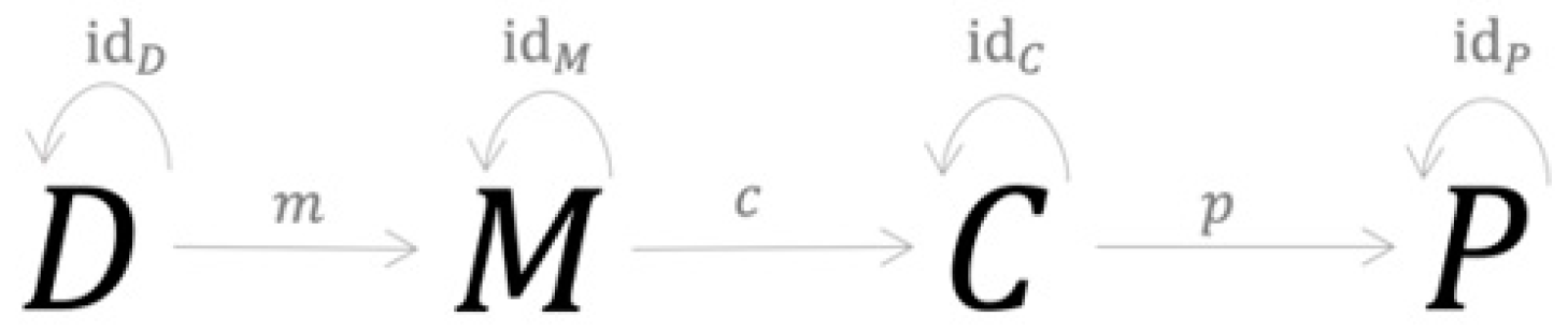
At this stage, four more morphisms, denoted with dD, idM, idC and idP, are introduced into the structure, as shown in Figure 2 below. They essentially send each object to itself, thus representing the objects’ identity morphisms. For example, the replacement operator which replaces one instance of an object with another instance can be used as an identity morphism. The resulting category , represents the process underlying current approaches to credit risk modeling.

Figure 2.
Category of the modeling process underlying current approaches.
From this structure, a specific approach to credit risk modeling is just a C-Instance of the category (R-instance ), represented by four elements and seven morphisms as shown in Figure 3.
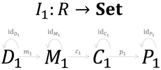
Figure 3.
A specific credit risk model is a C-Instance of category .
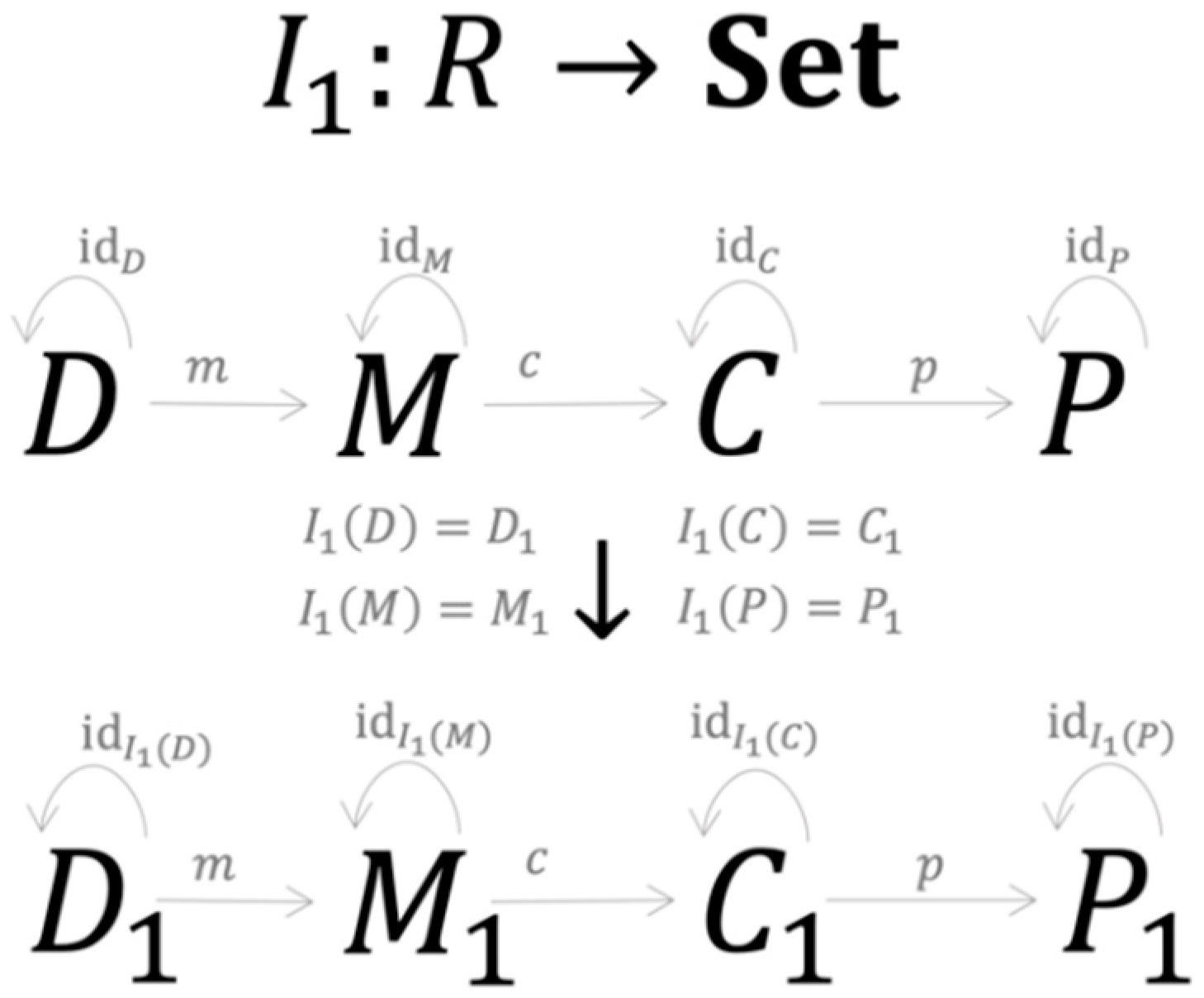
consists of the training and testing dataset sharing the same structure , with d being the number of sample points and representing n features associated with one of m credit classes . is a symbolic expression of the model’s structure in the form . Here is one of the k parameters obtained during the training process represented by the morphism , specifies the symbolic expression of and describes how are structured together. consists of the modeling results with structure where is a set of PDs obtained during the testing process, are elements of the confusion matrix (see Table A1) that are generated by the testing process , where is a true positive, FP is a false positive, FN is a false negative and TN is a true negative. consists of performance metrics generated by the morphism , which is a specific implementation of . Since the morphisms always generate unique results, they serve as the functional mapping between the set , and . Figure 4 summarises the set-valued functor performing the mapping process of the first R-instance.
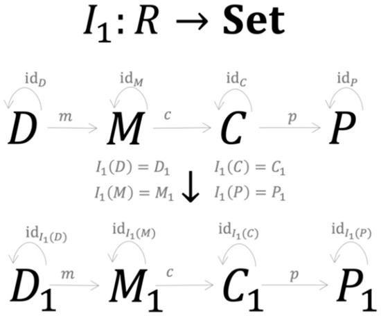
Figure 4.
The mapping process of the first R-instance.
Now suppose there is a second approach to credit risk modeling that can be represented as another R-instance , represented by four elements and seven morphisms (Figure 5).

Figure 5.
A specific credit risk model is a C-Instance of category .
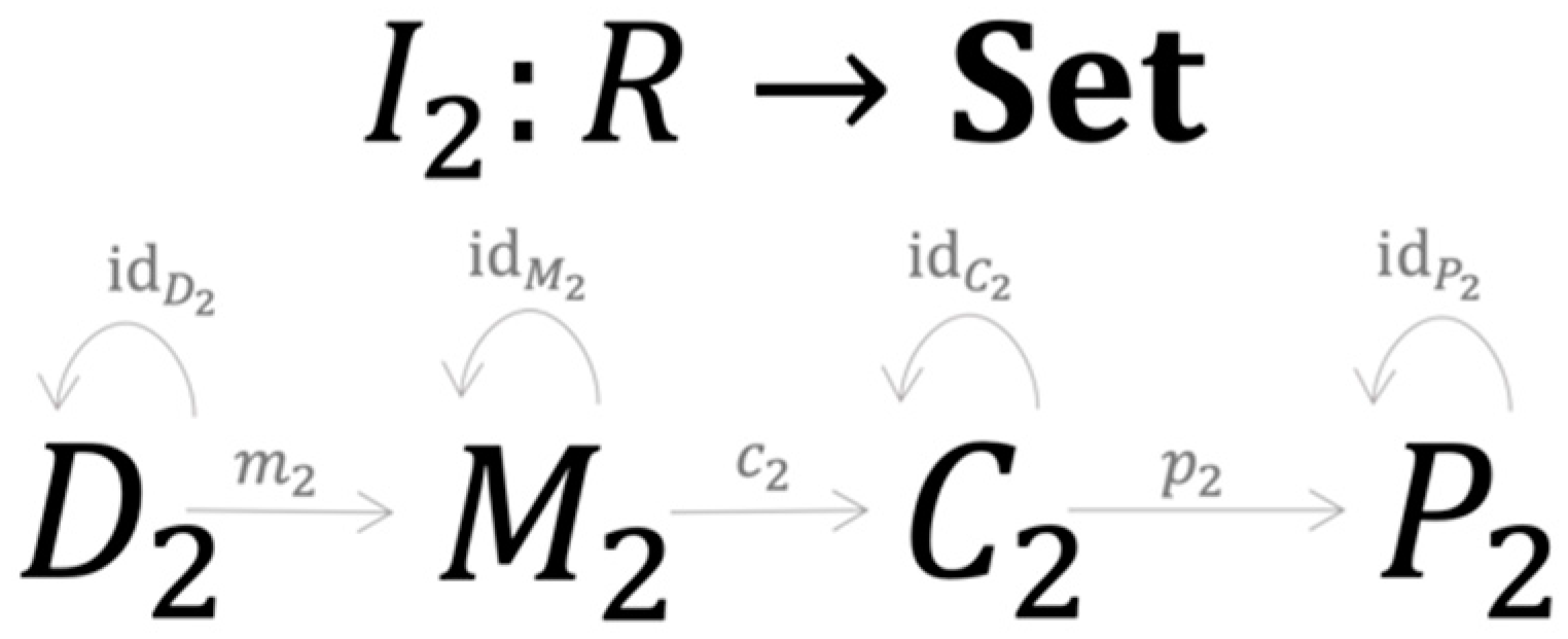
Assume the set-valued functor I2 performs the mapping as set out of Figure 6.
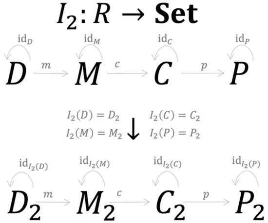
Figure 6.
The mapping process of the second R-instance.
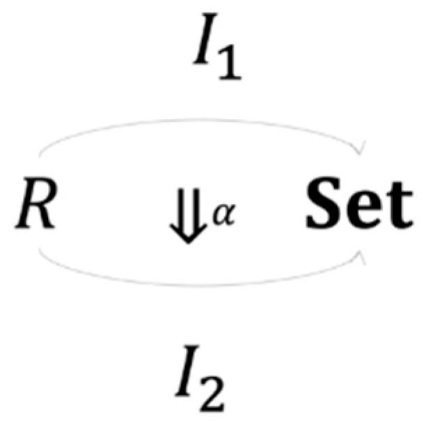
Since both R-instances have unique objects and morphisms that share the same exact structure, it follows that there is a natural transformation between them. Essentially, this natural transformation can be constructed as a term rewriting operation that replaces specific elements of one object in with a corresponding object in that satisfies the following
The existence of is warranted by the fact that any modeling approach would result in the same structures of their corresponding category and with the uniqueness of , and , while the operation ensures that the naturality condition holds for both and . More specifically, there is a natural isomorphism between the two instances and (Figure 7).

Figure 7.
Isomorphism between two R-instances.
The beauty of category theory thus comes from its design-as-proof feature. That is, given a proposition regarding relations between objects, as soon as a structure is properly constructed, the structure itself becomes a proof. The power lays in its capability to construct simple representations that captures the essence of credit risk modeling in a single concrete formalization (category), which may yield powerful insights into credit risk modeling that are difficult to identify using traditional comparative analysis of individual models usually seen in the literature. That is, different models and their underlying processes are just instances of the same modeling structures represented by a category. As a result, there is an equivalence between the various modeling processes that creates a performance boundary: Generalization power has meaning only within the categorical frame representing the modeling process. Consequently, two different credit risk models having the same categorical structure will on average deliver the same result if tested over all possible instances of the category. In practice, this process could go on indefinitely as new datasets would create new instances. Thus, representing credit risk modeling as a category yields a compact method to arrive at the equivalence concept without the burden of going through all possible empirical verifications.
2.2. Model Combination
A natural consequence of categorial equivalence is that combining different types of models can result in better and more consistent forecasting performance. Empirically, this has been observed in the literature (Dastile et al. 2020). Conceptually, for model combination to be effective, two conditions must be satisfied. First, since an instance of D determines C, the combination process must generate a new data instance having a structure different from the data initially used in the combination process. Second, the classification method adopted in the combination process must have a categorical structure different from the modeling process without combination. In this category, is decoupled from C. Instead, it is mapped to twice with the first morphism describing the usual process of individual model construction, as shown in Figure 8.
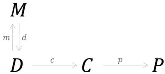
Figure 8.
A category of model combination based on a stacking process that avoids the equivalent trap.
The second morphism, , represents the process of generating a new data structure by using model combination. Performance is measured by applying a new morphism c, which is essentially a computational process, that maps the new data structure in to without going through any specific model. The morphism d does not necessarily generate a unique instance of since its construction depends on how the output of the individual models are combined, thus reducing the likelihood of categorical equivalence.
From a practical point of view, the main purpose of combining models based on the categorical framework is to address inconsistency and bias in classification performance. Inconsistency arises when models are sensitive to changes in the data structure, with their performance being valid only within specific contexts shaped by the structure and scope of the data. Bias is a result of the credit risk models used being sensitive to imbalance in default classes in the data. More specifically, models tend to be biased towards non-default prediction, generating performance that at first glance seems to be satisfactory overall but are poor in terms of capturing actual default outcomes. Bias is also a result of the tendency of modelers to focus on good overall prediction outcomes, with more attention paid to non-default outcomes and less attention to stability in performance (Abdou and Pointon 2011; Dastile et al. 2020; Lessmann et al. 2015). Unfortunately, it is common to find models showing high accuracy while failing to capture actual default outcomes.
The conceptual framework based on category theory provides an explanation as to why various ensemble (stacking) models proposed in the literature arrive at different conclusions regarding classification performance. Essentially, these models are caught in an equivalence trap. Ensemble models, despite their seemingly sophisticated assembling process, fuse the outputs of the base models either by majority voting or some type of linear weighted combination. In doing so, no new instance of the data structure D is created; all that has been achieved is an extension of the operation of the morphism c to cover the output combination process. As a result, the categorical structure remains the same as that of any other credit risk model with equivalent performance. In contrast, the stacking model proposed in this paper creates a new data structure D and at the same time a new instance of model choice M as a meta-classifier. It is the creation of M that effectively provides stacking models with a categorical structure that is identical to that of the typical credit risk model. However, the concept of an equivalence trap also applies in the situation, as shown in Figure 9.
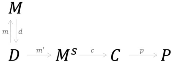
Figure 9.
A category representing the equivalence trap.
It is a category representing the equivalence trap often observed in typical stacking models. Essentially, the new data instance created by d can be used to train a new meta-classifier , which in turn brings the combination process back to the original structure of the modeling process.
The combination process proposed addresses this issue by considering two key issues. First, combining models, as the theoretical framework suggests, should first transform the initial feature space into a new data instance D with a structure different from the initial dataset, whilst still capturing information representing outcomes in the initial modeling phase. Second, the new data instance D should be transformed into PDs in a coherent and transparent manner without creating any new classifiers that puts the process into an equivalence trap. These considerations are supported by two conceptual constructs: Shannon’s information entropy and enriched categories, which are discussed next.
2.3. Shannon’s Information Entropy
Shannon (1948) proposed a concept called entropy to measure the amount of information created by an ergodic source and transmitted over a noisy communication channel. Noises here reflect uncertainty in how signals arrive at the destination and, for finite discrete signals, they are represented by a set of probabilities . Entropy H is defined as follows.
Judged by its construction, Shannon’s information entropy captures uncertainty in the communication as it deals with noise. Shannon (1948) considered this uncertainty to be the amount of information contained in the signals, thus conceptually establishing a link between uncertainty and information. Essentially, the entropy value tells us how much uncertainty must be removed by some process to obtain information regarding which signals arrive at the destination. Thus, it can said that the amount of information received from progressing through the process, results from the removal of the uncertainty that existed before the modeling process begun. The notion of the communication channel can be generalized to a finite event space that consists of n mutually exclusive and exhaustive events with their probabilities. The connection between entropy and information enables the creation of structures that effectively capture the information contained in the modeling process, a feature that will be exploited in the stacking model as a new data structure D used to enhance prediction. Other studies that similarly exploit the concept of entropy in risk assessment are Gradojevic and Caric (2016); Lupu et al. (2020) and Pichler and Schlotter (2020).
2.4. Enriched Categories
Another important construct used in the post-stacking classification process is the concept of enriched categories (Kelly 2005). Enriched categories replace the category of sets and mappings, which play a crucial role in ordinary category theory, by a more general symmetric monoidal closed category, allowing the results of category theory to be translated into a more general setting. Enriched categories are potentially an important analytical tool for classifying default outcomes. Essentially, the paired data of entropy value H and prediction output for the training data can be separated into two groups according to the classification class associated with each output. Each group can be viewed as a set of objects that is enriched in with their hom-object values, defined by whether they belong in the same group or not. A computational process is then constructed to obtain a borrower’s PD employing the following formula:
where is the likelihood that the applicant belongs to the default group and is the likelihood that the applicant belongs to the non-default group. Both and are computed using the Hamming and Manhattan distance. Thus, the combination model not only provides a new classification process but also a new method of estimating PD.
2.5. The Stacking Process
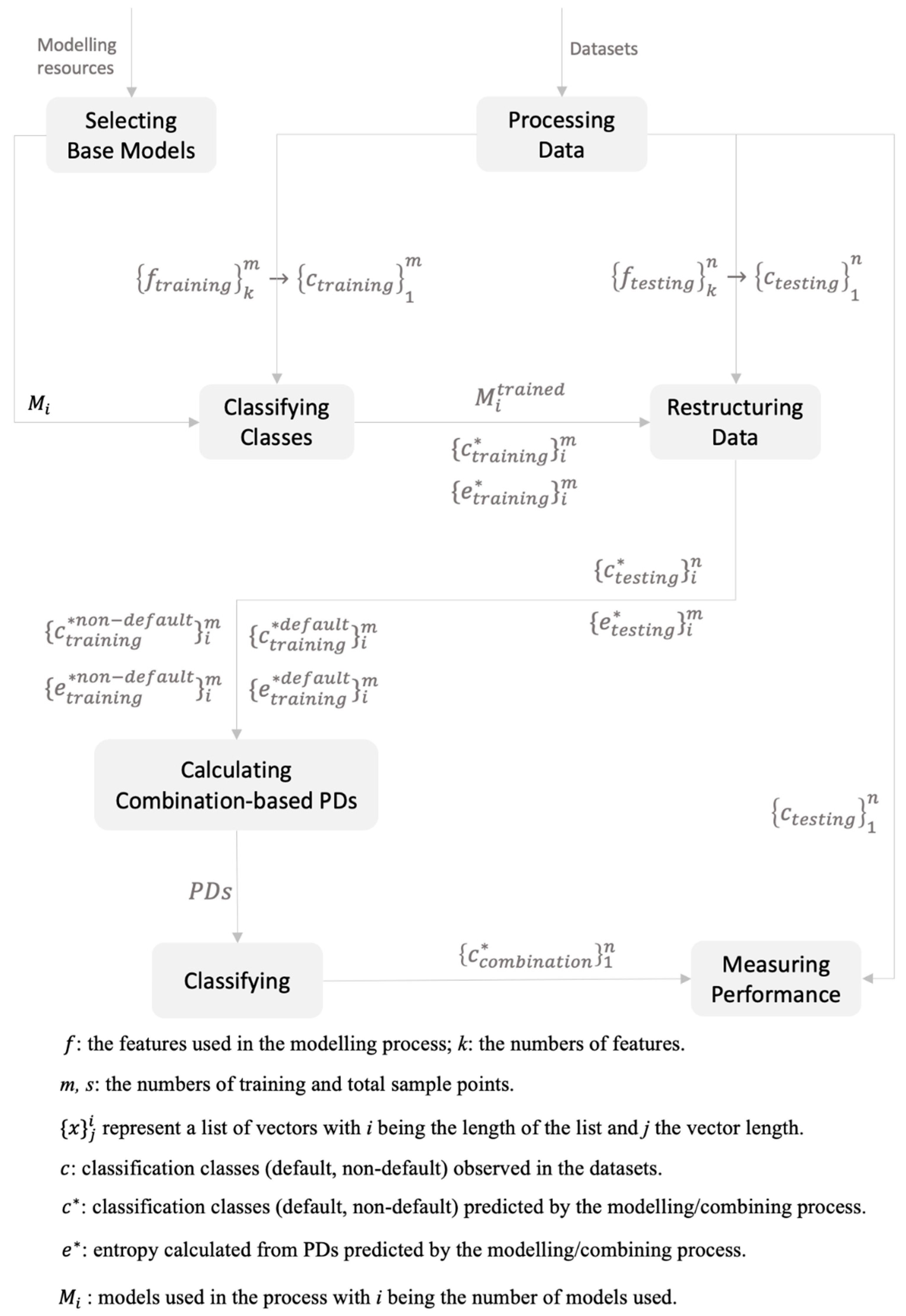
With the concepts of information entropy and enriched categories defined above, the stacking model is constructed as follows (see Figure A1 for a flow chart). First, several of the nine classifiers, consisting of a logistic regression and eight of the most popular supervised ML methods, are selected as the base models. Second, during the training and testing phases, the estimated PDs are used to compute the classifiers’ Shannon information entropy (H). The entropy value and the default classifications generated will then be paired to form a new (restructured) training dataset (D2). Next, employing the concept of enriched categories, final predictions are formed by assigning new testing samples into either the default group or the non-default group just constructed. Finally, the performance results of the stacking model are subjected to location tests to check for consistency and biasedness.
Several considerations differentiate the entropy-based stacking model proposed in this paper from the stacking models proposed by others (Doumpos and Zopounidis 2007; Wang et al. 2018). First, instead of selecting and processing the datasets carefully before training and testing a model only once on the dataset, as is usually done by others, the performance of the proposed entropy-based stacking model is assessed repeatedly on small randomly chosen non-overlapping subsets of the original dataset. Inherent class imbalance is utilized to make model comparison more realistic (Lessmann et al. 2015), enabling the construction of different data environments, and thus tests of performance inconsistency and bias. The data process ensures that each subsample will have a different structure regarding class ratio (default/non-default) and feature availability, especially categorical features. Further, performing many simulations allows for significance testing, which is preferred over making ad hoc judgements about average performance outcomes over limited rounds of tests. Thus, significance tests are a necessary complement to the usual average performance results reported by others. Statistical analyses of model performance are also proposed in Lessmann et al. (2015), but their non-parametric tests are performed on a sample of just 10.
The second consideration concerns model selection. Typically, the combination models proposed in the literature carefully select base models according to their performance on some testing data. Some combination of these models will then be benchmarked against all other models. The fact that their selection greatly determines the combination model’s overall performance suggests that the base model selection process is more critical than the combination process itself. In contrast, the entropy-based stacking model proposed in this paper seeks to prove that the combination process likely offers more consistent and less biased performance results, regardless of which base models are selected. In order to achieve this goal, the simulation process is carried out over 100 different data environments, with a different number of base models used in each simulation. Moreover, in each scenario, each sample is trained and tested on a different set of base models. Thus, the only element that remains invariant in each simulation is the reasoning process underlying the stacking model.
A final consideration is on demonstrating how a sound conceptual framework may enable quality model combination that both improves consistency and reduces bias in performance. It follows that the method can be applied to various situations without having to worry about the selection of the base models employed. Essentially, the approach avoids making any a priori judgments as to which combination of base models performs best. Comparison of this type often has little meaning since each study has its own unique data and optimization process (hyperparameters), both of which are difficult to replicate across data environments.
2.6. Base Models
Nine classifiers are used as the base models in the stacking process. Whilst not exhaustive, the models chosen are currently the most popular ones in the literature, covering most aspects of statistical and ML approaches, either as a standalone classifier or as part of a combination framework (Dastile et al. 2020; Lessmann et al. 2015; Teply and Polena 2020). Their key structures are discussed next.
i. Artificial Neural Networks
An Artificial Neural Network (ANN) is essentially a nested construct with each layer being represented by the same or a different function. In a mathematical form, a typical ANN model can be defined as follows (Barboza et al. 2017):
where n is the number of layers that transform the input feature into a final set of output features from which classification results are obtained by using the operation of . Typically, the inner nested function possesses the following form:
where i is the layer index spanning from 1 to n. The function is called an activation function, which usually has a non-linear form. Gradient descent techniques are used to obtain the parameter matrix and the vector through optimization processes constrained by some cost function (such as Mean Square Errors). The function is usually a scalar or a vector function that transforms previous layers’ output into the final classification results.
ii. Support Vector Machine
Support Vector Machine (SVM) is a parametric method that essentially puts the input features into a multi-dimension space and separates them into classes by a hyperplane , where is the parameter vector and is the feature vector. The classification decision has the following construct (Cortes and Vapnik 1995):
under the constraint of maximizing the distance or margin between the closest examples of two classes. In order to achieve this, the Euclidean norm of , which is , must be minimized, where n is the number of features.
iii. Logistic Regression
In a logistic regression model, the PD is computed as (Altman and Sabato 2007):
where , with representing a feature in the feature vectors and is the set of the model’s parameters obtained by the maximum likelihood estimation on the training dataset.
iv. Decision Trees
A decision tree is a kind of acyclic graph in which splitting decisions are made at each branching node where a specific feature of the feature vector is examined. The left branch of the tree will be followed if the value of the feature is below a specific threshold; otherwise, the right branch will be followed. At each split, the process calculates two entropy value (Safavian and Landgrebe 1991) described as follows:
where and are two sets of split labels and is the decision tree with the initial value defined as . For each case, the process will go through all pairs of features and thresholds and it will choose the ones that minimize the split entropy:
which is the weighted average entropy at a leaf node. The classification will then be made using the average value of the chosen labels along the selected nodes.
v. Random Forest
This is essentially an ensemble of decision trees, with each tree built on bootstrapped samples of the same size (Breiman 2001). Each tree works on a set of features chosen randomly and classes are the generated for these features. The overall classification is obtained through majority voting of the trees’ decisions. This approach reduces the likelihood of correlation of the trees since each tree works on a different set of features. Correlation will thus make majority voting more effective. By using multiple samples of the original dataset, variance of the final model is reduced. As a result, overfitting is also reduced.
vi. Gradient Boosted Tree
This method uses an adaptive strategy that starts with a simple and weak model and then the method learns about its shortcomings before addressing them in the next model, which is often more sophisticated (Chen and Guestrin 2016). Examples incorrectly classified by the previous classifier would be assigned larger weights in the next classifier. The classifiers’ outputs will then be ensembled in the following construct to yield the final classification result:
where n is the total number of classifiers and , which is learned during the training process, is the weight of the classifier .
vii. Naïve Bayes
In a default classification problem, Naïve Bayes (NB) is essentially a decision process based on the following construct (Rish 2001):
where 1 represents non-default status and −1 default status. The conditional probability is computed according to the Bayesian rule with and , which is assumed to follow a normal distribution with mean and covariance matrices computed on the default and non-default sample groups constructed from the training dataset. The model assumes that the features are mutually independent.
viii. Markov model
In a Markov model, each feature vector is treated as a member in a sequence and the probability distribution for the feature vectors given a credit classification class could be estimated from the training data as described as follows:
where is the feature vector that requires probability estimation, is the set of the feature vectors preceding and is a credit classification class. The cardinality of determines how far the model would look back to obtain information for the next prediction. In this context, a cardinality of n would result in a so called n-gram Markov model (Brown et al. 1992). If , a Naïve Bayes model is generated, which will be discussed shortly. At test time, the probability for each class given a feature vector is computed according to Bayes’ theorem where is computed from the Markov model that is just derived in the training process and is a class defined prior to the start of the modeling process.
ix. k-Nearest Neighbor
This is a non-parametric method in the sense that no functional form needs to be constructed for the classification purpose (Henley and Hand 1996). The process learns how to assign a new sample point to a group of known examples and then to generate classification based upon a majority voting of the classes observed in the group. The modeling process is represented by the following constructs:
where denotes the distance between elements in the group and the new example. Typically, the Euclidean or Mahalanobis distance is used in the model.
2.7. Method of Comparison
Before discussing the relative performance of the proposed stacking model, it is desirable to consider an appropriate method of gauging agreement between prediction and observation. The first performance metric employed is the Matthew Coefficient Correlation (MCC). It is the preferred benchmarking criteria for binary confusion matrix evaluation as it avoids issues related to asymmetry, loss of information and bias in prediction (Matthews 1975). MCC computed as follows:
A key advantage of MCC is that it immediately provides an indication as to how much better a given prediction is than a random one: MCC = 1 indicates perfect agreement, MCC = 0 indicates a prediction no better than random, whilst MCC = −1 indicates total disagreement between prediction and observation.
In addition to MCC, Accuracy is employed as an overall classification performance metric that captures consistency of the model in terms of overall predictive capability. It is computed as follows:
This metric avoids the class asymmetry issue by looking at overall prediction performance, but often suffers from prediction bias caused by the imbalance problem with non-default predictions likely to account for most of the results. A very high TN with low TP results in high Accuracy without accurately capturing poor prediction outcomes for the default class.
The final performance metric is Extreme Bias, which captures the situation in which a model fails to generate a correct classification of a credit class. It is described as follows:
where
Essentially, the Extreme Bias of a model is the number of times the model generates an MCC = 0 (no better than random). This measure reveals situations in which mean Accuracy is high, but the prediction is extremely biased.
3. Data
Credit risk analysis is performed on two major datasets (see Table 1). The first is the peer-to-peer loans dataset of the Lending Club (Lending Club 2020). The scale of the platform’s dataset and the maturity of loan portfolios (212,280 loans from 2007 to 2013) makes it an ideal sample for testing various types of credit risk models (Chang et al. 2015; Malekipirbazari and Aksakalli 2015; Teply and Polena 2020; Tsai et al. 2009).

Table 1.
Data Description.
Although much smaller in size (~30,000 loans for 2005), the second is the credit card clients dataset from Taiwan (Yeh 2006) used by Yeh and Lien (2009) to benchmark the predictive power of various credit classification models.
4. Empirical Results
Table 2 and Table 3 summarize the relative performance of the proposed stacking model for the Lending Club’s peer-to-peer loans dataset and the Taiwanese credit card clients dataset, respectively. Reported are the mean values of MCC and Accuracy as well as Extreme Bias count (zero value MCC count) over 100 simulations. Also reported is the standard deviation of the MCC values, giving an indication of performance consistency, and the significance test of differences (p < 10%) in mean MCC values (equal to or greater than) between the stacked model and the base models selected. The prediction statistics reported for the stacking models are for two to nine base models, where both the subsets of the original dataset and the base models are chosen at random (non-overlapping).
Table 2.
Modeling Results for the Lending Club Peer-to-Peer Loans Dataset.
Table 3.
Modeling Results for Taiwanese Credit Card Clients Dataset.
Distinctly, the proposed stacking model delivers better performance in default prediction, relative to the individual base models, and for both data sets. The mean MCC is always higher for the stacking model that for the individual base models, with significance tests strongly supporting this conclusion. Most notably, the stacking model achieves consistently better performance across the various data environments as indicated by the low standard deviation of MCC. In contrast, the performance of the individual base models is highly inconsistent, as indicated by the high standard deviation of MCC. Amongst the nine individual base models, Naïve Bayes provides the best average prediction performance (MCC = 0.14) for the Lending Club peer-to-peer loans dataset, whilst Random Forest provides the best average performance (MCC = 0.33) for the Taiwanese credit card clients dataset.
Compared to the individual base models, the stacking model provides the best overall performance, with the mean MCC value exceeding that of any of the individual base models selected, with an overall agreement between prediction and observation twice as high for the Taiwanese credit card clients dataset compared to the Lending Club’s peer-to-peer loans dataset. While in a few cases the performance of the stacking model appears similar to the base model selected (as indicated by the mean MCC value), the individual base models always experience high Extreme Bias. For example, for the Taiwanese credit card clients dataset, while the mean MCC (about 0.32) for the Random Forest model is similar to that of the proposed stacking model, the Random Forest model experiences high Extreme Bias (4–8%), with the prediction of the base model no better than random.
Again, in terms of Accuracy, the stacking model delivers highly and consistent performance across all data environments. Mean Accuracy of the stacking model tends to fluctuate close to 0.79 across all data environments. In contrast, for the individual base models, mean Accuracy fluctuates significantly between 0.66 to 0.84. None of the individual base models show consistency in performance across the data environments.
Whilst the stacking model does not provide the highest mean Accuracy in all cases, in all cases it experiences the lowest Extreme Bias. This renders the Accuracy measure somewhat inapt in terms of judging prediction performance. At best, Accuracy should be used as a complement to MCC, with its usefulness viewed in terms of satisfactory consistency. That is, a good model should deliver relatively stable Accuracy.
5. Discussion
The computational effort in this paper has been in running a large number of simulations to capture different data environments. The results of the simulations presented in the previous section support the proposed stacking model in terms of providing more consistent performance across data environments and less biased performance in terms of default classification. Unlike previous studies, which have been unable to settle which base model exhibits superior default classification performance across multiple data environments (Ala’raj and Abbod 2016a; Lessmann et al. 2015; Li et al. 2018; Xia et al. 2018), this paper shows that careful selection of base models is not necessary. The performance of the proposed stacking model remains high and consistent despite changes in the number and type of base model used or the data used to train the model on. In other words, the reasoning process itself is somewhat agnostic as to which base model is selected, thus enabling replication of the stacking method in a wide range of situations, allowing meaningful comparative analysis across multiple data environments.
In essence, the power of the conceptual construct based on category theory lies in its capability to construct simple representations that captures the essence of credit risk modeling in a single concrete formalization (a category). It yields powerful insights into credit risk modeling that are difficult to identify using traditional comparative analysis of individual base models frequently adopted in the literature. That is, different models and their underlying processes are just instances of the same modeling structures represented by a category. As a result, there is an equivalence (trap) between the various modeling processes, creating a performance boundary. That is, generalization power has meaning only within the categorical frame representing the modeling process. Consequently, two seemingly different credit risk models that have the same categorical structure will on average produce identical results if tested over all possible instances of the category. In practice, this process could continue indefinitely as new datasets create new instances. This has been clearly demonstrated by the empirical results, showing poor performance persistence of the base models selected across different data environments. It follows that representing credit risk modeling as a category yields a compact method to arrive at the equivalence concept without the burden of having to go through all possible empirical verifications, as revealed by the literature.
6. Conclusions
Two motivations underly the use of category theory to credit risk modeling. First, it serves as a powerful tool to construct an inward view of our own reasoning processes in credit risk modeling. By using this view, invariant structures emerge and form a basis on which construction of the relationship between seemingly unrelated models can be created. Furthermore, category theory enables these structures to form relationships with new conceptual constructs in fields unrelated to credit risk modeling. This unique capability enlarges the space of potential modeling solutions, resulting in improved default prediction performance. Second, categorical constructs result in new perspective on the meaning of risk beyond PDs. From this perspective, credit risk is not just a quantification of specific features but also a property emerging out of a network of relationships between various modeling processes represented by enriched categories. Thus, credit risk assessment is no longer an endeavor carried out with an isolated model; it has become as a network phenomenon. Creating the theoretical framework is, therefore, a novel contribution to the current body of literature.
By focusing on credit risk through these structures, the equivalence implication was better understood and a stacking model was introduced with two new structures, enriched categories and information entropy. The empirical results showed that the stacking framework’s performance remained robust despite changes in data environments and selection of the base models, thus enabling more objective replication. The conceptual structures, seemingly disconnected, turned out to be perfect companions in the stacking model.
That said, there are some limitations to the paper. The first issue relates to substantial computational overhead associated with implementing the proposed stacking model. Whilst there is no doubt that keeping the per-unit processing cost low is an important concern to credit providers, advances in supercomputing are likely to push computational costs down considerably soon. The second issue relates to the performance of the stacking model which could be tested more extensively by application to more datasets and by comparing with a larger number of base models, including deep learning and unsupervised learning. This could not only create a more dynamic testing environment but also provide more transparency for replication purposes. A unified stacking and dynamic model selection framework would enable more extensive statistical tests of performance, an objective that has so far been absent from the literature but could be a fruitful avenue for further research. A final issue of concern is that the focus on constructing classification models has value only at the time of application. The focus of risk managers is undoubtedly on the development of credit risk models that provide lenders with on-going predictive diagnosis of clients’ credit risk status. However, this would require a richer dataset.
While the approach embraced in this paper is essentially exploratory in its nature, it is likely to raise more questions than provide answers on sound credit risk modeling.
Author Contributions
Conceptualization, C.S.T.; methodology, C.S.T. and R.N.; software, C.S.T.; analysis, C.S.T.; writing—original draft preparation, P.V.; writing—review and editing, C.S.T., D.N., R.N. and P.V. All authors have read and agreed to the published version of the manuscript.
Funding
This research received no external funding.
Institutional Review Board Statement
Not applicable.
Informed Consent Statement
Not applicable.
Data Availability Statement
Not applicable.
Conflicts of Interest
The authors declare no conflict of interest.
Appendix A. Key Definitions in Category Theory
Definition A1.
A category
has the following elements:
- A collection of objects denoted as Ob();
- For every two objects c and d, there is a set that consists of morhphims from or ;
- For every object , there is a morphism , called the identity morphism on . For convenience, is used instead of ;
- For every three objectsand morphismsand, there is a morphism, called the composite ofand .
- These elements are required to satisfy the following conditions:
- For any morphism, withand , which is called the unitality condition;
- For any three morphisms,and, the following are equal: . This is called the associativity condition.
Definition A2.
The category Set is defined as follows:
- Ob(Set) is the collection of all sets;
- If S and T are sets, then Set(X,Y) =, where is a function;
- For each set S, the identity functionis given byfor each ;
- Givenand, their composite function is .
- Since these elements satisfy the unitality and associativity conditions, Set is indeed a category.
Definition A3.
A functor between two categoriesand, denoted , is defined as follows:
- For every object, there is an object ;
- For every morphismin, there is a morphismin .
- These elements are required to satisfy the following conditions:
- For every object , ;
- For any three objects,andand two morphisms,, and, the equationholds in .
Definition A4.
A-instance of the categoryis functor .
Definition A5. 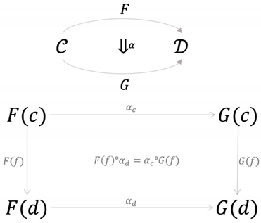
Letandbe categories andbe functors. A natural transformation is defined as follows:
- For each object, there is a morphismin, called the c-component of , that satisfies the following naturality condition;
- For every morphismin , the following equation holds.
A natural transformationis called a natural isomorphism if each componentis an isomorphism in. The naturality condition can be represented as follows.
The concept of natural transformation plays an important role in understanding relations between two categories. It describes how the two functorsandcan be used to as two representations of categoryinside with the natural transformation connecting these two representations using the morphisms in .
In order to arrive at enriched categories, the following definitions apply.
Definition A6.
Letandbe sets. A relation betweenandis a subset. A binary relation onis a relation betweenand, i.e. a subset of .
Definition A7.
A preorder relation on a setis binary relation on, denoted as , that satisfies the following two properties:
- Reflexivity: ; and
- Transitivity: Ifand, then .
- The preorder can be denoted as .
Definition A8.
A symmetric monoidal structure on a preorderhas the following two elements:
- An element, called the monoidal unit;
- A function , called the monoidal product.
- These elements must satisfy the following four properties:
- Monotocity: for all ;
- Unitality: for all, the equations hold;
- Associativity: for all holds;
- Aymmetry: for all holds.
- This structure is called a symmetric monoidal preorder and is denoted as .
Definition A9.
A symmetric monoidal structure on a preorder has the following two elements:
- An element , called the monoidal unit;
- A function , called the monoidal product.
- These elements must satisfy the following properties:
- Monotocity: for all ;
- Unitality: for all, the equations hold;
- Associativity: for all holds;
- Symmetry: for all holds.
- This structure is called a symmetric monoidal preorder denoted as. Let, the structurecam be developed with representing the AND operation defined in the following matrix.
It is trivial to show that this structure forms a symmetric monoidal structure.false true false false false true false True
Definition A10.
Letbe a symmetric monoidal preorder. A -category has the following two elements:
- A set , elements of which are called objects;
- For every two objects, there is an element , called the hom-object.
- These elements must satisfy the following two properties:
- For every object, ;
- For every three objects, all .
- Hence, it can be said thatis enriched in .
Table A1.
Confusion Matrix.
Table A1.
Confusion Matrix.
| Prediction | |||
| Default | Non-Default | ||
| Actual | Default | TP | FN |
| Non-Default | FP | TN | |
Notes: “Positive (P)” is the term used to describe a prediction of default and “Negative (N)” for a prediction of non-default outcome. “True (T)” means the actual data agrees with the prediction, whilst “False (F)” means the data does not agree with the prediction.

Figure A1.
Flow Diagram of the Proposed Entropy-based Stacking Model.
Figure A1.
Flow Diagram of the Proposed Entropy-based Stacking Model.
References
- Abdou, Hussein A., and John Pointon. 2011. Credit scoring, statistical techniques and evaluation criteria: A review of the literature. Intelligent Systems in Accounting, Finance and Management 18: 59–88. [Google Scholar] [CrossRef] [Green Version]
- Abellán, Joaquin, and Carlos J. Mantas. 2014. Improving experimental studies about ensembles of classifiers for bankruptcy prediction and credit scoring. Expert Systems with Applications 41: 3825–30. [Google Scholar] [CrossRef]
- Ala’raj, Maher, and Maysam F. Abbod. 2016a. Classifier’s consensus system approach for credit scoring. Knowledge-Based Systems 104: 89–105. [Google Scholar] [CrossRef]
- Ala’raj, Maher, and Maysam F. Abbod. 2016b. A new hybrid ensemble credit scoring model based on classifiers consensus system approach. Expert Systems with Applications 64: 36–55. [Google Scholar] [CrossRef]
- Altman, Edward I. 1968. Financial ratios, discriminant analysis and the prediction of corporate bankruptcy. The Journal of Finance 23: 589–609. [Google Scholar] [CrossRef]
- Altman, Edward I., and Gabriele Sabato. 2007. Modeling credit risk for SMEs: Evidence from the U.S. Market. Abacus 43: 332–57. [Google Scholar] [CrossRef]
- Asquith, Paul, David W. Mullins, and Eric D. Wolff. 1989. Original issue high yield bonds: Aging analyses of defaults, exchanges, and calls. The Journal of Finance 44: 923–52. [Google Scholar] [CrossRef]
- Aster, Richard C., Brian Borchers, and Clifford H. Thurber. 2018. Parameter Estimation and Inverse Problems, 3rd ed. Amsterdam: Elsevier Publishing Company. [Google Scholar]
- Barboza, Flavio, Herbert Kimura, and Edward Altman. 2017. Machine learning models and bankruptcy prediction. Expert Systems with Applications 83: 405–17. [Google Scholar] [CrossRef]
- Breiman, Leo. 2001. Random forests. Machine Learning 45: 5–32. [Google Scholar] [CrossRef] [Green Version]
- Brown, Peter F., Vincent J. Della Pietra, Peter V. Desouza, Jenifer C. Lai, and Robert L. Mercer. 1992. Class-based n-gram models of natural language. Computational Linguistics 18: 467–80. [Google Scholar]
- Chang, Shunpo, Simon D-O Kim, and Genki Kondo. 2015. Predicting default risk of lending club loans. CS229: Machine Learning, 1–5. Available online: http://cs229.stanford.edu/proj2018/report/69.pdf (accessed on 24 January 2021).
- Chen, Tianqi, and Carlos Guestrin. 2016. XGBoost: A scalable tree boosting system. Paper presented at the 22nd ACM SIGKDD International Conference on Knowledge Discovery and Data Mining, San Francisco, CA, USA, August 13–17; New York, NY, USA: Association for Computing Machinery, pp. 785–794. [Google Scholar] [CrossRef] [Green Version]
- Cortes, Corinna, and Vladimir Vapnik. 1995. Support-vector networks. Machine Learning 20: 273–97. [Google Scholar] [CrossRef]
- Dastile, Xolani, Turgay Celik, and Moshe Potsane. 2020. Statistical and machine learning models in credit scoring: A systematic literature survey. Applied Soft Computing 91: 106263. [Google Scholar] [CrossRef]
- Doumpos, Michael, and Constantin Zopounidis. 2007. Model combination for credit risk assessment: A stacked generalization approach. Annals of Operations Research 151: 289–306. [Google Scholar] [CrossRef]
- Eilenberg, Samuel, and Saunders MacLane. 1945. General theory of natural equivalences. Transactions of the American Mathematical Society 58: 231–94. [Google Scholar] [CrossRef] [Green Version]
- Finlay, Steven. 2011. Multiple classifier architectures and their application to credit risk assessment. European Journal of Operational Research 210: 368–78. [Google Scholar] [CrossRef] [Green Version]
- Gradojevic, Nikola, and Marko Caric. 2016. Predicting systemic risk with entropic indicators. Journal of Forecasting 36: 16–25. [Google Scholar] [CrossRef] [Green Version]
- Henley, William, and David J. Hand. 1996. A k-nearest-neighbour classifier for assessing consumer credit risk. Journal of the Royal Statistical Society: Series D (The Statistician) 45: 77–95. [Google Scholar] [CrossRef]
- Hsieh, Nan-Chen, and Lun-Ping Hung. 2010. A data driven ensemble classifier for credit scoring analysis. Expert Systems with Applications 37: 534–45. [Google Scholar] [CrossRef]
- Jonkhart, Marius J. L. 1979. On the term structure of interest rates and the risk of default: An analytical approach. Journal of Banking & Finance 3: 253–62. [Google Scholar] [CrossRef]
- Joy, Maurice O., and John O. Tollefson. 1978. Some clarifying comments on discriminant analysis. Journal of Financial and Quantitative Analysis 13: 197–200. [Google Scholar] [CrossRef]
- Kelly, Max G. 2005. Basic Concepts of Enriched Category Theory. London Mathematical Society Lecture Note Series 64; Cambridge: Cambridge University Press. Reprinted as Reprints in Theory and Applications of Categories 10. First published 1982. [Google Scholar]
- Lawrence, Edward C., Douglas L. Smith, and Malcolm Rhoades. 1992. An analysis of default risk in mobile home credit. Journal of Banking & Finance 16: 299–312. [Google Scholar] [CrossRef]
- Lending Club. 2020. Peer-to-Peer Loans Data. Available online: https://www.kaggle.com/wordsforthewise/lending-club (accessed on 24 November 2020).
- Lessmann, Stefan, Bart Baesens, Hsin-Vonn Seow, and Lyn C. Thomas. 2015. Benchmarking state-of-the-art classification algorithms for credit scoring: An update of research. European Journal of Operational Research 247: 124–36. [Google Scholar] [CrossRef] [Green Version]
- Li, Wei, Shuai Ding, Yi Chen, and Shanlin Yang. 2018. Heterogeneous ensemble for default prediction of peer-to-peer lending in China. IEEE Access 6: 54396–406. [Google Scholar] [CrossRef]
- Lupu, Radu, Adrian C. Călin, Cristina G. Zeldea, and Iulia Lupu. 2020. A bayesian entropy approach to sectoral systemic risk modeling. Entropy 22: 1371. [Google Scholar] [CrossRef]
- Malekipirbazari, Milad, and Vural Aksakalli. 2015. Risk assessment in social lending via random forests. Expert Systems with Applications 42: 4621–31. [Google Scholar] [CrossRef]
- Martin, Daniel. 1977. Early warning of bank failure: A logit regression approach. Journal of Banking & Finance 1: 249–76. [Google Scholar] [CrossRef]
- Matthews, Ben W. 1975. Comparison of the predicted and observed secondary structure of T4 phage lysozyme. Biochimica et Biophysica Acta (BBA)-Protein Structure 405: 442–51. [Google Scholar] [CrossRef]
- Mcleay, Stuart, and Azmi Omar. 2000. The sensitivity of prediction models to the non-normality of bounded and unbounded financial ratios. British Accounting Review 32: 213–30. [Google Scholar] [CrossRef]
- Ohlson, James A. 1980. Financial ratios and the probabilistic prediction of bankruptcy. Journal of Accounting Research 18: 109–31. [Google Scholar] [CrossRef] [Green Version]
- Pichler, Alois, and Ruben Schlotter. 2020. Entropy based risk measures. European Journal of Operational Research 285: 223–36. [Google Scholar] [CrossRef] [Green Version]
- Rish, Irina. 2001. An empirical study of the naive Bayes classifier. Paper presented at the IJCAI 2001 Workshop on Empirical Methods in Artificial Intelligence, Seattle, WA, USA, August 4–6; vol. 3, pp. 41–46. [Google Scholar]
- Safavian, Stephen R., and David Landgrebe. 1991. A survey of decision tree classifier methodology. IEEE Transactions on Systems, Man, and Cybernetics 21: 660–74. [Google Scholar] [CrossRef] [Green Version]
- Santomero, Anthony. M., and Joseph D. Vinso. 1977. Estimating the probability of failure for commercial banks and the banking system. Journal of Banking & Finance 1: 185–205. [Google Scholar] [CrossRef]
- Shannon, Claude E. 1948. A mathematical theory of communication. The Bell System Technical Journal 27: 379–423. [Google Scholar] [CrossRef] [Green Version]
- Tam, Kar Yan. 1991. Neural network models and the prediction of bank bankruptcy. Omega 19: 429–45. [Google Scholar] [CrossRef]
- Teply, Petr, and Michal Polena. 2020. Best classification algorithms in peer-to-peer lending. North American Journal of Economics and Finance 51: 100904. [Google Scholar] [CrossRef]
- Tsai, Ming-Chun, Shu-Ping Lin, Ching-Chan Cheng, and Yen-Ping Lin. 2009. The consumer loan default predicting model. An application of DEA–DA and neural network. Expert Systems with Applications 36: 11682–90. [Google Scholar] [CrossRef]
- Vassalou, Maria, and Yuhang Xing. 2004. Default Risk in Equity Returns. The Journal of Finance 59: 831–68. [Google Scholar] [CrossRef]
- Wang, Maoguang, Jiayu Yu, and Zijian Ji. 2018. Personal credit risk assessment based on stacking ensemble model. Paper presented at the 10th International Conference on Intelligent Information Processing (IIP), Nanning, China, October 19–22. [Google Scholar]
- Wolpert, David H. 1992. Stacked generalization. Neural Networks 5: 241–59. [Google Scholar] [CrossRef]
- Xia, Yufei, Chuanzhe Liu, Bowen Da, and Fangming Xie. 2018. A novel heterogeneous ensemble credit scoring model based on stacking approach. Expert Systems with Applications 93: 182–99. [Google Scholar] [CrossRef]
- Yeh, I-Cheng. 2006. Default of Credit Card Clients Data Set. Department of Information Management, Chung Hua University, Taiwan. Available online: https://archive.ics.uci.edu/ml/datasets/default+of+credit+card+clients (accessed on 24 November 2020).
- Yeh, I-Cheng, and Che-hui Lien. 2009. The comparisons of data mining techniques for the predictive accuracy of probability of default of credit card clients. Expert Systems with Applications 36: 2473–80. [Google Scholar] [CrossRef]


Publisher’s Note: MDPI stays neutral with regard to jurisdictional claims in published maps and institutional affiliations. |
© 2021 by the authors. Licensee MDPI, Basel, Switzerland. This article is an open access article distributed under the terms and conditions of the Creative Commons Attribution (CC BY) license (https://creativecommons.org/licenses/by/4.0/).