Abstract
We use a dynamic factor model to provide a semi-structural representation for 101 quarterly US macroeconomic series. We find that (i) the US economy is well described by a number of structural shocks between two and five. Focusing on the four-shock specification, we identify, using sign restrictions, two policy shocks, monetary and fiscal, and two non-policy shocks, demand and supply. We obtain the following results. (ii) Both supply and demand shocks are important sources of fluctuations; supply prevails for GDP, while demand prevails for employment and inflation. (ii) Monetary and fiscal policy shocks have sizable effects on output and prices, with no evidence of crowding-out of private aggregate demand components; both monetary and fiscal authorities implement important systematic countercyclical policies reacting to demand shocks. (iii) Negative demand shocks have a large long-run positive effect on productivity, consistently with the Schumpeterian “cleansing” view of recessions.
Keywords:
demand; supply; fiscal policy; monetary policy; sign restrictions; structural factor model JEL Classification:
C32; E32; E52; F31
1. Introduction
How many shocks drive the business cycle? What is the relative importance of supply and demand disturbances? What are the effects of macroeconomic policies? These questions have been and still are at the core of the research in macroeconomic since the answer is key to assessing competing theories of the business cycle and the implied policy recommendations.
Since Sims (1980) seminal paper, structural Vector Autoregressive models (SVAR) have been a major tool to address the questions above. Such models replaced large scale econometric models, their main advantage being that they do not require the imposition of “incredible” identifying restrictions. Over the last three decades, the SVAR literature has substantially contributed to improve our knowledge of macroeconomic dynamics, providing evidence often used as a guideline by both policymakers and theorists. Nonetheless, we believe that SVAR models have an important limitation: the amount of information that they can handle is perforce small, owing to the so-called “curse of dimensionality”. The relevance of this information issue is stressed in several papers, including Quah (1990), Sims (1992), Lippi and Reichlin (1994), Bernanke and Boivin (2003), and Bernanke et al. (2005). If, as plausible, both policy makers and private economic agents base their decisions on all of the available macroeconomic information, structural shocks should be innovations with respect to a large information set, perhaps larger than the one that can be included in a standard VAR.
An alternative to SVAR models is represented by a new generation of large dimensional structural models: the “generalized” or “approximate” dynamic factor models introduced by Forni et al. (2000), Forni and Lippi (2001), Stock and Watson (2002a), (2002b), and recently proposed for structural economic analysis (Stock and Watson 2005; Forni et al. 2009). Such models have been successful in solving well known VAR puzzles (Bernanke et al. 2005; Forni and Gambetti 2010; Alessi and Kerssenfischer 2019). Their key advantage is that they combine a large number of macroeconomic variables with a reduced number of macroeconomic shocks. Two basic features distinguish large factor models from old-fashioned large scale models. First, identification can be reached in just the same way as in VAR models, without relying on “incredible” restrictions. Second, the forecasting performance is good (Stock and Watson 2002a, 2002b; Altissimo et al. 2010).1
In this paper, we use a large structural factor model to address the questions raised at the beginning of this introduction. Specifically, we apply the model and the estimation method of Forni et al. (2009) to 101 US quarterly series, covering the pre-zero lower bound sample period 1959-I to 2007-IV. Following Uhlig (2005), we adopt an identification scheme based on inequality constraints. Such constraints are milder than the traditional zero restrictions commonly used in the VAR literature, in that only the sign of the impulse response functions at a few specific lags are imposed. Sign restrictions are particularly appropriate in our data-rich framework, since they can be imposed on a broad set of variables and this, in turn, is likely to deliver a better characterization of the shocks. The main difference with the existing literature, which has been focusing on the identification of a single shock, see for instance Forni and Gambetti (2010) and Alessi and Kerssenfischer (2019), and the main novelty is that we provide a global identification of the model and this allows us to provide a semi-structural representation of the US economy. In this way we can assess the relative importance for economic fluctuations of various types of economic disturbances.
As a first step in our analysis we address the fundamental question: how many shocks drive macroeconomic fluctuations? This question has largely been ignored in the empirical literature, probably because it is not meaningful within a VAR framework, where the number of economic shocks is determined by the number of variables included in the model. Using some popular information criteria, we find that the US economy can be well described by a number of shocks between 2 and 5. The finding is at odds with theories relying on a single source of fluctuations, like early RBC models. Furthermore, the numbers are slightly smaller than the number of shocks typically included in modern DSGE models, like for instance Smets and Wouters (2007) which considers seven structural shocks.
We then focus on a four-shock specification and identify two non-policy shocks, demand and supply, and two policy shocks, monetary and fiscal. All shocks are normalized as expansionary by imposing positive effects on output (GDP and industrial production). We further impose that supply reduce prices, whereas the other three shocks raise prices (CPI and GDP deflator). Moreover, we impose that expansionary monetary policy reduces the federal funds rate and expansionary fiscal policy raises federal deficit.
Our main findings are the following: (i) Both supply and demand shocks explain a considerable fraction of the fluctuations in real variables. However, their relative importance depends on the specific variable considered. Supply shocks explain most of GDP volatility, while demand shocks prevail for employment and other labor market variables. Demand shocks are less persistent than supply shocks and their long-run effect on GDP is not significant. Concerning inflation, both supply and demand have relevant effects; however, demand shocks prevail, particularly in the long-run. (ii) Policy is important. Discretionary monetary policy shocks have sizable effects on output and prices and are responsible for the early 1980s recession and disinflation. Discretionary fiscal policy shocks have sizable effects on GDP and do not have important crowding-out effects on private consumption and investment, with the sole exception of residential investment. As for systematic policy, there is evidence of a strong countercyclical response of both monetary and fiscal authorities to demand and, to a lesser extent, supply shocks. (iii) Positive demand shocks have a persistent negative effect on labor productivity. This finding, while being at odds with most of the business cycle literature, is consistent with a stream of empirical and theoretical work concerning the interactions between growth and cycle and the Schumpeterian view of recessions as providing a cleansing mechanism for reducing organizational inefficiencies and resource misallocations.
2. Theory
In the present section we provide a presentation of our model and estimation procedure. For additional details see Forni et al. (2009), FGLR from now on.
2.1. The Factor Model
We assume that each variable of our macroeconomic data set is the sum of two mutually orthogonal unobservable components, the common component and the idiosyncratic component :
The idiosyncratic components are poorly correlated in the cross-sectional dimension (see FGLR, Assumption 5 for a precise statement). They arise from shocks or sources of variation which considerably affect only a single variable or a small group of variables; in this sense, we could say that they are not “macroeconomic” shocks. For variables related to particular sectors, like industrial production indexes or production prices, the idiosyncratic component may reflect sector specific variations (with a slight abuse of language we could say “microeconomic” fluctuations); for strictly macroeconomic variables, like GDP, investment or consumption, the idiosyncratic component must be interpreted essentially as a measurement error.
The common components are responsible for the main bulk of the co-movements between macroeconomic variables, being linear combinations of a relatively small number r of factors , not depending on i:
The dynamic relations between the macroeconomic variables arise from the fact that the vector of the common factors follows the VAR relation
where R is a matrix and is a q-dimensional vector of orthonormal white noises, with . Such white noises are the “common” or “primitive” shocks or “dynamic factors” (whereas the entries of are the “static factors”).2
2.2. Identification
Representation (4) is not unique, since the impulse-response functions and the related primitive shocks are not identified. In particular, if H is any orthogonal matrix, then in (3) is equal to , where and , so that , with . However, assuming mutually orthogonal structural shocks, post-multiplication by is the only admissible transformation, i.e., the impulse–response functions are unique up to orthogonal transformations, just like in structural VAR models (FGLR, Proposition 2). As a consequence, structural analysis in factor models can be carried on along lines very similar to those of standard SVAR analysis.
To be precise, let us assume that economic theory implies a set of restrictions on the impulse–response functions of some variables, the first with no loss of generality. Let us write such functions in matrix notation as . Given any non-structural representation
along with the relation
if theory-based restrictions on are sufficient to obtain H, then is uniquely determined for any i (just identification).
In the present paper, however, we do not identify uniquely the shocks and the impulse–response functions; rather, following Uhlig (2005), we identify a distribution of shocks and related impulse–response functions by imposing a set of sign restrictions on the impulse-response functions themselves. Formally, let be the coefficient of the term of degree k of . We impose for , and for , , where , , and are sets of integers. The precise set of restrictions that we impose in the present paper is discussed below.
A quite natural parameterization of the orthogonal matrices H is given by the hyperspherical coordinates of the unit sphere of dimension , i.e., , being a w-dimensional vector of angles such that , , . Given the non-structural representation , the sign restrictions above define an admissible region on the unit sphere, such that for satisfies such inequalities. Following Uhlig (2005) we assume that the true shocks and impulse–response functions are associated with a point with uniform probability density in the region . This in turn implies upper and lower bounds and a probability density for each coefficient of the impulse–response functions .
2.3. Estimation
As for estimation, we proceed as follows. First, starting with an estimate of the number of static factors, we estimate the static factors themselves by means of the first ordinary principal components of the variables in the data set, and the factor loadings by means of the associated eigenvectors. Precisely, let be the sample variance-covariance matrix of the data: our estimated loading matrix is the matrix having on the columns the normalized eigenvectors corresponding to the first largest eigenvalues of , and our estimated factors are .
Second, we set a number of lags and run a VAR() with to get estimates of and the residuals , say and .
Now, let be the sample variance–covariance matrix of . As the third step, having an estimate of the number of dynamic factors, we obtain an estimate of a non-structural representation of the common components by using the spectral decomposition of . Precisely, let , , be the j-th eigenvalue of , in decreasing order, the diagonal matrix with as its entry, the matrix with the corresponding normalized eigenvectors on the columns. Setting , our estimated matrix of non-structural impulse–response functions is
To account for estimation uncertainty, we adopt the following standard non-overlapping block bootstrap technique. Let be the matrix of data. Such matrix is partitioned into S sub-matrices (blocks), , of dimension , being the integer part of .4 An integer between 1 and S is drawn randomly with reintroduction S times to obtain the sequence . A new artificial sample of dimension is then generated as and the corresponding impulse–response functions are estimated. A set of non-structural impulse–response functions is obtained by repeating drawing and estimation.
Finally, we obtain a distribution of impulse–response functions by imposing our sign identification restrictions. Precisely, we proceed as follows. For each artificial sample we compute the corresponding non-structural impulse–response functions . Then we draw N times a vector of angles with dimension from a uniform distribution in the range , , and retain the related as long as they satisfy the sign restrictions. This gives a distribution of estimated ’s. We get a point estimate and the related confidence bands by retaining the median along with the relevant percentiles of such a distribution.5
2.4. Discussion
FGLR is a special case of the generalized dynamic factor model proposed by (Forni et al. 2000, 2005) and Forni and Lippi (2001). Such model differ from the traditional dynamic factor model of Sargent and Sims (1977) and Geweke (1977) in that the number of cross-sectional variables is infinite and the idiosyncratic components are allowed to be mutually correlated to some extent, along the lines of Chamberlain (1983), Chamberlain and Rothschild (1983), and Connor and Korajczyk (1988). Closely related models have been studied by (Stock and Watson 2002a, 2002b, 2005), (Bai and Ng 2002, 2007), Bai (2003), and Bernanke et al. (2005).
Large statistical factor models are compatible with a variety of economic models, including both neo-classical and Neo-Keynesian DSGE models, augmented with measurement errors (see Sargent and Sims 1977; Sargent 1989; Altug 1989; Ireland 2004 and the literature mentioned therein). However, in the present work we do not propose a fully developed economic model characterized by “deep” parameters. Rather, our approach is very much in the spirit of Sims (1980) and the “structural” VAR literature. Our impulse response functions can indeed be labeled as “semi-structural”, rather than “structural”: while not being reduced form coefficients, they are still a mixture of behavioral and policy parameters, so that we cannot tell, say, what would happen in absence of systematic fiscal or monetary policy. The results of the present paper should then be interpreted essentially as stylized facts, conditional on the identified shocks.
Why using a structural factor model rather then a structural VAR? Factor models impose a considerable amount of structure on the data, implying restricted VAR relations among variables (see Stock and Watson (2005) for a comprehensive analysis). In this sense, they are less general than VAR models. On the other hand, factor models have a few advantages that can be important in the present context.
First, within a factor model we can study how many shocks are there in the macro economy, an economic question which has been largely ignored in the literature simply because it does not even make sense within the statistical VAR framework, where the number of shocks is necessarily equal to the number of variables that the econometrician chooses to include in the data set. However we believe that investigating the number of shocks driving the economy is of crucial importance since it can provide evidence that can be used as guidance for building macroeconomic models.
Second, being much more parsimonious in terms of parameters, factor models can handle a much larger amount of information. The data set used in this paper, for instance, is made up of 101 variables. A VAR model with the same number of series would have too many parameters to estimate, given the number of observations available in the time dimension.
Having a large data set is important for three reasons. First, we can study the impulse response functions of virtually all relevant macro variables within a unified framework. We exploit this opportunity here by showing results for key macro variables.
Second, it enables us to impose identifying restrictions on several variables, reducing the region of admissible impulse response functions and causing the confidence bands to shrink. For instance, we identify an expansive demand shock by imposing positive effects on output and prices; as output series we use both GDP and the industrial production index, while prices are measured by both the GDP deflator and the CPI.
Last, but not least, large information is likely to produce better results. The relevance of the information issue is stressed in several influential papers, including Quah (1990) and Sims (1992). If, as is reasonable, central banks and private economic agents base their decisions on all of the available macroeconomic information, structural shocks should be innovations with respect to a large information set, perhaps larger than the one that can be included in a standard VAR model. In fact, large dimensional factor models have proven useful in solving well known VAR puzzles (Bernanke et al. 2005; Forni and Gambetti 2010).
The discussion above could call to mind the old controversy concerning the properties of large and small econometric models. In this respect, it should be observed that a major difference between the large econometric models prevailing fifty years ago and the large factor models proposed in the modern literature is that the former had bad forecasting performances, whereas the latter have been proven successful in forecasting (Stock and Watson 2002a, 2002b).
3. Identifying the Structural Shocks
In this section, we describe the data, identify the number of structural shocks and describe the set of inequality restrictions used to estimate the impulse response functions.
3.1. Data, Data Treatment and Specification of the Number of Factors
The data set used in this paper is made up of 101 US quarterly series, covering the period 1959-I to 2007-IV. Most series are taken from the FRED data base. A few stock market and leading indicators are taken from Data Stream. Some series have been constructed by ourselves as transformations of the original FRED series. The series include both national accounting data like GDP, investment, consumption and the GDP deflator, which are available only at quarterly frequency, and series like industrial production indices, CPI, PPI, and employment, which are produced monthly. Monthly data have been temporally aggregated to get quarterly figures.
As required by the model, the data were transformed to obtain stationarity. Stationarity tests were taken seriously, so that prices and nominal variables were taken in second differences of logs, rather than first differences of logs, and interest rates in first differences, rather than in levels. With these transformations all variables are stationary according to both the ADF and the KPSS tests.6
The full list of variables along with the corresponding transformations is reported in the Appendix A.
The number of static factors r was set to 15 as suggested by the popular criterion IC2 (), proposed by Bai and Ng (2002).
Finally, the number of lags p to include in the VAR which is part of our estimation procedure was set to 2, the average of AIC (3 lags) and BIC (1 lag).
3.2. How Many Macroeconomic Shocks?
Determining the number of shocks, besides being an important step for the specification of our model, has intrinsic economic interest. For instance, early real business cycle models assume the existence of just one supply shock driving economic fluctuations, whereas, on the other extreme, Smets and Wouters (2007) propose a new Keynesian DSGE seven structural shocks. In the present factor model framework we have both tests and consistent information criteria which can provide useful indications for economic modeling.7
The number of shocks can be determined by a few consistent information criteria. Here we use three groups of criteria, proposed by Amengual and Watson (2007), Bai and Ng (2007) and Hallin and Liska (2007). The criterion by Amengual and Watson in the version (with and ) gives 4 primitive factors. The four criteria of Bai and Ng (2007), namely and , give 5, 4, 4, and 3 shocks, respectively (with and ).8 Finally, the log criterion proposed by Hallin and Liska (2007) gives 2 and 4 shocks. In summary, information criteria do not provide a unique result, the number of shocks being between 2 and 5. We conclude in favor of a four-shock specification which is the specification suggested by all of the criteria.
3.3. Identifying Restrictions
We identify three demand shocks and one supply shock. We think particularly appealing a characterization of the demand shocks as “discretionary fiscal policy”, “discretionary monetary policy”, and “private demand” (independent of discretionary monetary policy).
To characterize such shocks we adopt the following definitions. The expansionary monetary policy shock is defined as a shock having a positive effect on both output and prices, but a negative effect on the federal funds rate. We expect that expansionary monetary policy enlarges money aggregates, but prefer not to impose such a restriction as part of the definition of the shock, in order to keep the definition itself as simple as possible.
An obvious logical implication of the above characterization is that positive private demand and fiscal policy shock do not have a negative effect on the federal funds rate. Despite this, we do not impose such constraint, since in the present framework imposing a non-negative effect is equivalent to imposing a significant positive effect, which would be unnecessarily restrictive. Interestingly, it turns out that the restriction is satisfied confirming the non-monetary nature of the two shocks.
The expansionary fiscal policy shock is defined as a shock having a positive effect on output, prices and the real federal deficit.9 Again, a logical implication is that the expansionary private demand shock does not have a positive effect on the federal deficit. Indeed, we expect a significant negative effect, but do not impose such constraint.
Most of the restrictions above are imposed on the first three coefficients of the impulse response functions, i.e., on the impact effect as well as the effects delayed by one and two quarters. However, there are two exceptions. First, we do not impose any restriction on the impact effects of monetary policy on output and prices. This is because both output and prices might react to monetary policy with some delay. In the structural VAR literature such a delayed reaction is commonly assumed to identify monetary policy (see Christiano et al. 1999 for a review). Here it is not assumed, the impact response can be zero or different from zero, the data will speak. Second, the positive effect of expansionary fiscal policy on the federal deficit, output and prices are imposed only on lag 1 and 2. The reason is the following. On one hand, the effects of fiscal policy decisions on public expenditures or receipts are often delayed by several months as discussed in the fiscal foresight literature, see Leeper et al. (2013). On the other hand, the sign and the size of the impact effects of such decisions on output and prices are not obvious. For instance, consumers might anticipate a larger income in the near future, but also a reduced public expenditure or higher taxes in the medium run. If public expenditure is delayed and consumption does not increase on impact, output and prices do not necessarily increase contemporaneously.
Summing up, the supply shock increases GDP and industrial production and reduces the GDP deflator and the CPI at lags 0, 1, and 2; the private demand shock increases GDP, industrial production, the GDP deflator and the CPI at lags 0, 1, and 2; the monetary policy shock reduces the federal funds rate at lags 0, 1, and 2 and increases GDP, industrial production, the GDP deflator and the CPI at lags 1 and 2; the fiscal policy shock increases GDP, industrial production, the GDP deflator, the CPI and the real federal deficit at lag 2.
Such constraints are not sufficient per se to guarantee that all shocks are well defined. In addition we need that (i) the private demand shock does not reduce the federal fund rate for at least one of the lags 0, 1, or 2; (ii) the private demand shock does not increase the real federal deficit at lag 2; (iii) at least one of the following conditions holds: (iii.1) the monetary policy shock does not increase the federal deficit at lag 2, (iii.2) the fiscal policy shock does not reduce the federal funds rate for at least one of the lags 0, 1, or 2. Conditions (i) and (ii) are needed to characterize the private demand shock, whereas condition (iii) is needed to distinguish monetary from fiscal policy.
4. Results
In this section, we present our main findings. We begin by showing a few results validating our identification scheme. Then we show results concerning the size and the timing of the effects of supply and demand shocks. Finally, we address policy issues and discuss the effects of demand on productivity.
4.1. Validating the Identification of Structural Shocks
The purpose of this subsection is to validate our identification procedure along two dimensions. First, we check whether the inequality restrictions are sufficient to get a full characterization of the three demand shocks, i.e., conditions (i)–(iii) above are satisfied. Second, we show that the response of some relevant variables conform to the consensus view.
The first column of Figure 1 shows the mean impulse response functions (solid lines) of the federal funds rate to the four shocks, along with the 68% confidence bands (gray areas). First, both a positive demand shock and an expansionary fiscal policy shock generate an immediate positive effect on the federal funds rate. Hence conditions (i) and (iii.2) are satisfied. Second, deficit significantly reduces at all horizons after a demand shock, thus ensuring condition (ii), whereas it is essentially unaffected by the monetary policy shock, the effects being remarkably small and not significant at all horizons, consistently with condition (iii.1). The results suggest that the identifying restrictions are sufficient for a proper characterization of the three demand shocks.
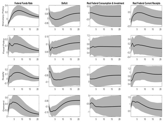
Figure 1.
Impulse-response functions. Solid line point estimate, gray areas 68% confidence bands.
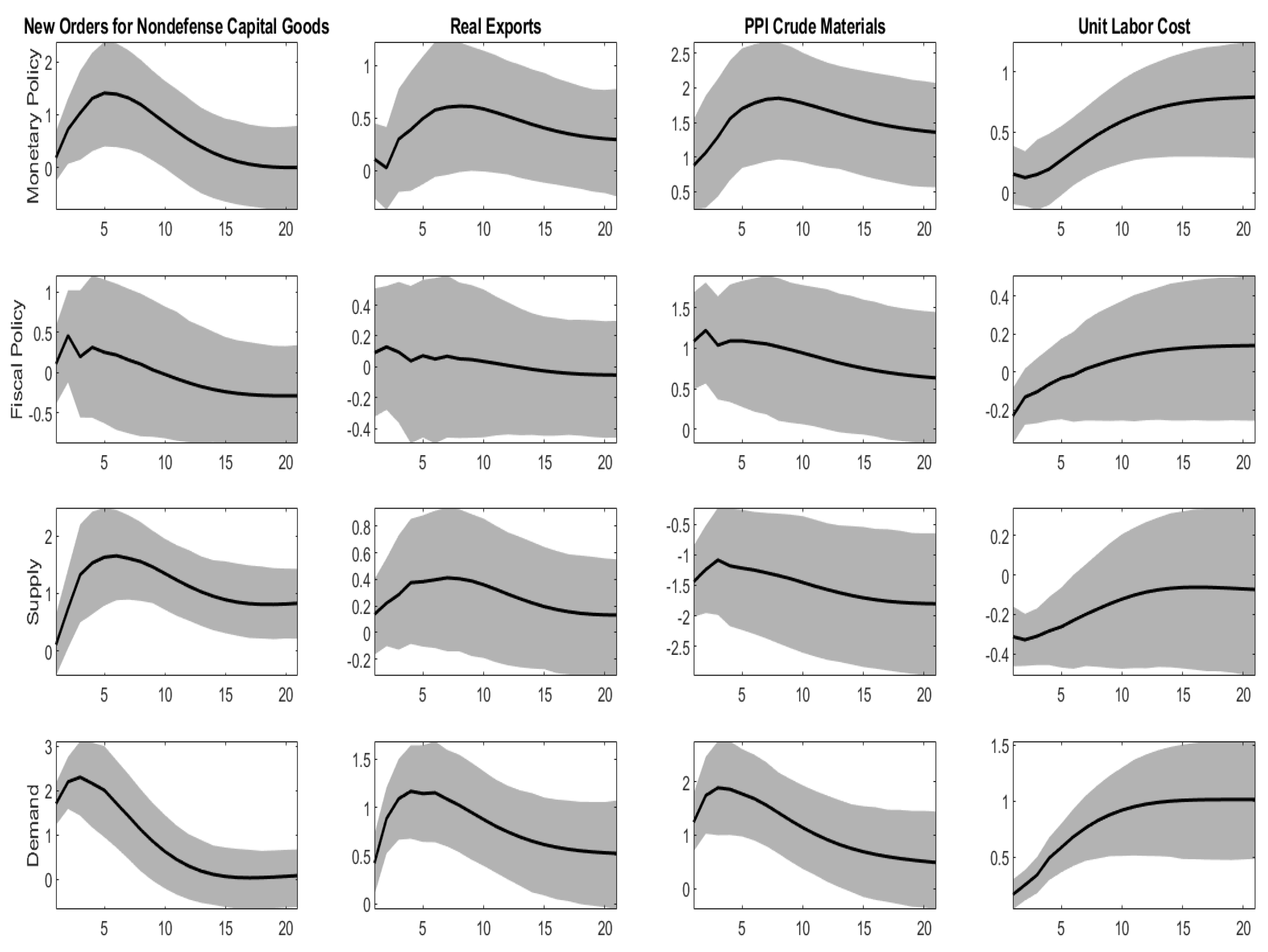
Next we show the effect of our identified shocks on a few selected variables, in order to verify whether they conform to some basic features emerging from previous literature and to gain additional insights about their sources and their nature. The non-policy demand shock is the only one that affects significantly, on impact, both new orders and real exports, see Figure 2. Furthermore, the demand shock is the primary source of unexpected change in investment on impact, explaining almost one half of the forecast error variance at lag 0 (as against 20% of consumption, see Table 2 below). While new orders and investment mainly capture factors that increase domestic demand, real exports indicates that the shock is also related to external factors.

Figure 2.
Impulse-response functions. Solid line point estimate, gray areas 68% confidence bands.
As far as the supply shock is concerned, Figure 2 shows that both the producer price index of crude materials and the unit labor cost immediately and significantly fall, indicating that the supply shocks are partly made up of unexpected changes in some key production costs. Moreover, the shock has a large and significant positive impact on labor productivity (Figure 6), in line with the consensus view that supply shocks include an important technological component.
4.2. The Relative Importance of Demand and Supply Shocks
Table 1 shows the variance decomposition of (the stationary transformation of) some selected series. Columns 2 to 6 report the percentages of variance explained by the monetary policy shock (MP), the fiscal shock (FS), the supply shock (S), the non-policy demand shock (D), and the two policy shocks jointly (MP+FS).

Table 1.
Variance decomposition.
Supply shocks explain around 46% of the variance of GDP growth, being more important for consumption than for investment. Such result is in line with King et al. (1991). Policy shocks account for about 35%, while non-policy demand shocks explain only 18%. While policy shock have similar effects for both investment and consumption, non-policy demand seems to matter more for investment than consumption.
The balance between demand and supply shock, however, changes substantially when other variables are considered. Regarding industrial production, for instance, the contribution of supply reduces to 27%, as against 45% of non-policy demand. This is consistent with the fact that, as already noted, private-demand shocks primarily concern investment and exports, which mainly involve goods, rather than services.
The importance of demand is even larger for labor market variables, such as employment, hours worked or the unemployment rate. Focusing on employment, for instance, the percentage of variance accounted for by supply shocks reduces to 21%, while the one accounted for by non-policy demand shocks is raised up to 48%. Such a large difference between employment and GDP variance decomposition is probably due to the technology component of supply shocks. While demand affects output mainly through employment changes, supply largely affects GDP through the important impact on productivity already noted above.
Table 2 displays the decomposition of the forecast error variance at different horizons. The previous results are confirmed. In particular, supply shocks explain most of GDP variance, while demand shocks prevail as far as employment is concerned. On impact (k = 0) such dichotomy is particularly pronounced: supply shocks explain 57% of output as against 8% of employment, whereas non-policy demand accounts for 63% of employment but only 13% of output. From Table 2 it also emerges clearly that, in the long run, the effects of non-policy demand on all real variables reduce, while the effects of supply increase, consistently with the consensus view that supply shocks are more persistent.
Table 2.
Forecast error variance decomposition at different horizons.
Considering prices, the bulk of fluctuations in the GDP deflator is accounted for by the three demand shocks, which, taken together, account for about 80% of the variance of the series. The result is confirmed by Table 2: demand shocks account for about 65%, 73%, and 87% at horizons 0, 4, and 24 quarters, respectively.
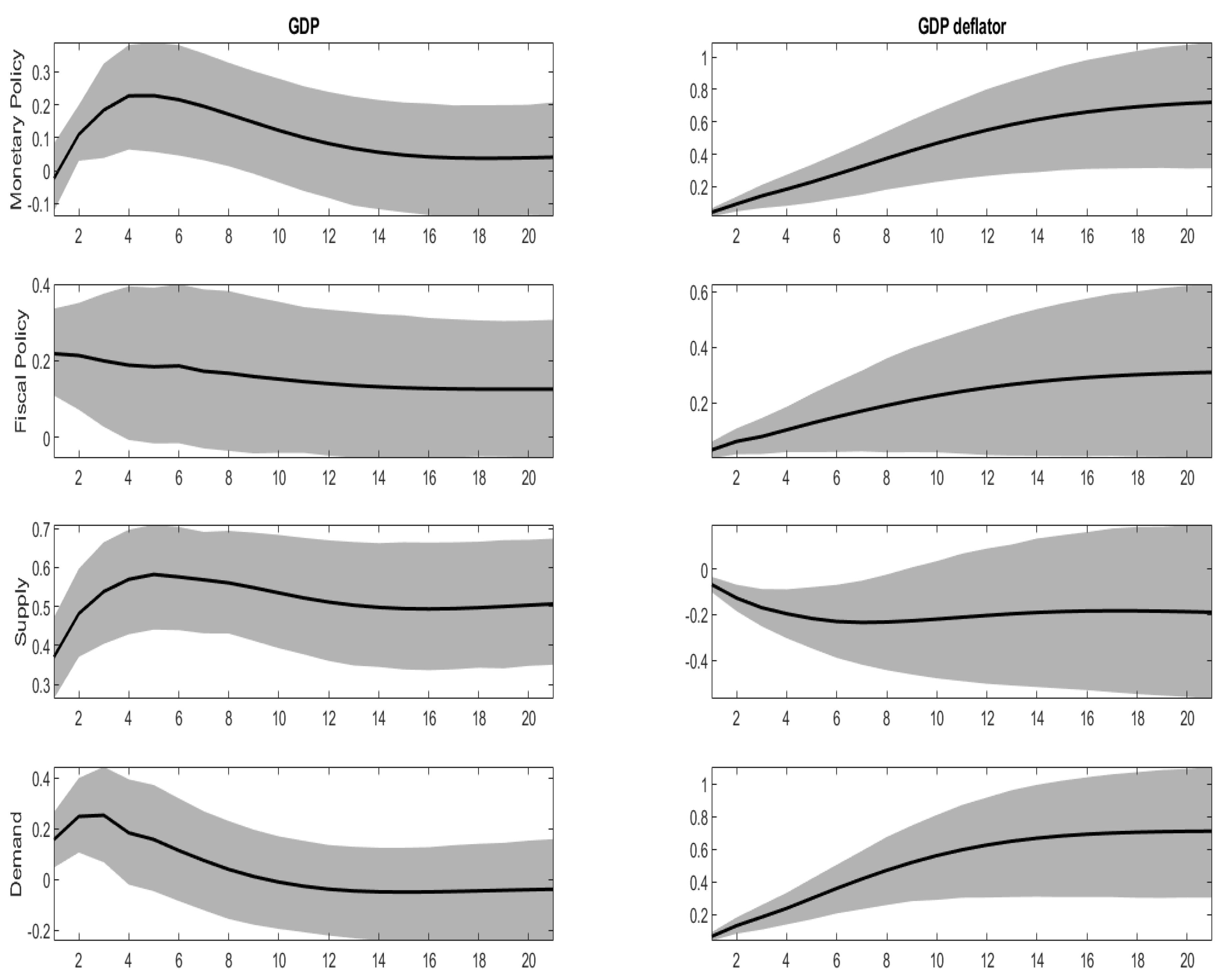
Figure 3 plots the impulse response functions of GDP and the GDP deflator to the four shocks. Several interesting features emerge. First, all of the shocks except monetary policy affect significantly output on impact. The effect is particularly large for supply shocks. Second, both fiscal policy and non-policy demand shocks have temporary effects on output, whereas the supply shock has large and significant permanent effects. Long-run neutrality of demand on output is consistent with mainstream theory and is adopted as an identifying assumption in the SVAR literature, starting with the seminal work of Blanchard and Quah (1989). Third, despite this, demand is not long-run neutral on all real variables, persistence being particularly pronounced for employment. We will come back to this point below. Fourth, the GDP deflator significantly increases at all horizons for the three demand shocks and reduces significantly at all horizons for the supply shock.

Figure 3.
Impulse response functions. Solid line point estimate, gray areas 68% confidence bands.
As far as consumption and investment are concerned, see Figure 4 and Figure 5, the supply shock is the only one generating permanent effects on the two variables. The three demand shocks produce temporary effects. The non-policy demand shock, consistent with the variance decomposition discussed above, turns out to be especially important for fluctuations in investment, which are hump-shaped and persistent. On the contrary the effects on consumption are relatively short lived and not-significant except in the very short run.
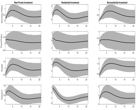
Figure 4.
Impulse-response functions. Solid line point estimate, gray areas 68% confidence bands.
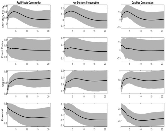
Figure 5.
Impulse-response functions. Solid line point estimate, gray areas 68% confidence bands.
In summary, both supply and demand shocks are important sources of macroeconomic fluctuations, but the relative importance differs substantially across variables. Supply prevails for GDP, whereas demand prevails for employment and prices. Demand shocks are less persistent than supply shocks for all real variables. Finally, policy shocks have sizable effects on output and prices.
4.3. The Role of Monetary and Fiscal Policy
This sub-section addresses three key policy questions. First, what and how big are the effects of monetary and fiscal discretionary policies on GDP and prices? Second, are consumption and investment crowded out by discretionary fiscal policy? Third, do monetary and fiscal authorities react systematically to macroeconomic shocks?
Monetary policy and fiscal shocks account for about 14% and 20% of the fluctuations in GDP, respectively, (see Table 2). Fiscal policy shocks appear to be slightly more important than monetary policy shocks especially in the short run (24% versus 4% at k = 0). This is due to the different shape of the impulse response functions. The response of GDP to a monetary policy shock is persistent but has a nearly zero impact effect while the response to a fiscal policy shock reaches the maximal level on impact and is relatively short lived. As far as inflation is concerned, monetary and fiscal policy shocks explain around 30% and 12% of the volatility of the growth rates of the GDP deflator, respectively. Percentages are similar at all horizons.
Figure 4, line 2, plots the impulse response functions of investment, residential investment and nonresidential investment to a unit variance fiscal policy shock. The responses of nonresidential and residential investment are somewhat different. The former increases significantly on impact, whereas the latter does not. In the long run the effects are not significant for both variables. In conclusion, private investments are not displaced by an expansionary fiscal policy.
The second row of Figure 5 plots the impulse response functions of consumption, durable consumption and nondurable consumption to a unit variance fiscal policy shock. The three responses have similar shapes, with a positive impact effect, followed by a reduction. The impact effect is much larger for durables (0.3% as against 0.06%). On aggregate the impact effect is small (around 0.1% as compared to 0.3% of investment). All effects are not significant. Such picture is different to that of Blanchard and Perotti (2002), where consumption is found to considerably increase, but is also different to those of Ramey and Shapiro (1998) and Ramey (2011), where consumption is found to significantly fall. The small reaction of nondurable consumption (and hence aggregate consumption) to both the fiscal policy and the non-policy demand shocks seems in line with standard permanent income theory, provided that, at least in part, consumers correctly perceive the increase of income as transitory. The positive sign of the response is in contrast with theoretical predictions from standard RBC models. Overall, there is no evidence of crowding-out of private expenditure after a fiscal policy shock.
Let us now focus on the dynamics of systematic monetary and fiscal policy, i.e., how policy reacts to non-policy shocks. Let us consider first monetary policy. After both a non-policy demand and a fiscal policy shock the federal funds rate immediately increases (Figure 1). The effect is significant in both cases, although, from a quantitative point of view, the effect of the non-policy demand shock is about two times larger than that of fiscal policy. This suggests a substantially degree of countercyclical behavior of monetary policy, which is consistent with standard Taylor rules implying systematic policy reaction to increases in prices and output.
On the contrary, the federal funds rate responds negatively to the supply shock on impact, although the effect is not significant. However, the effect becomes positive and significant after about one year, converging to 0.4% in the long run. Taking a standard Taylor rule as the benchmark, the result indicates that while in the very short run the opposite effects of output and inflation offset each other, in the long run the effects on inflation reduce and the federal funds rate seems to follow the pattern of output.
Let us now come to systematic fiscal policy (Figure 1). Government spending essentially does not react to monetary policy and supply shocks, the effect of such shocks being not significant at any horizon. On the contrary, the non-policy demand shock induces a strong countercyclical behavior of fiscal authorities. Government spending reduces significantly at all horizons by about 0.5%. We can get some idea of the effects of such policy by looking at Table 1. The fraction of variance of GDP growth explained by the non-policy demand shock (18%) is substantially smaller than the one of its components: investment (36%), consumption (18%), and government expenditure (31%). This is attributable to the negative comovement of private demand components and government spending.
There is little evidence, however, of an active behavior of fiscal authorities on the receipt side, since current receipts essentially follow fluctuations in GDP. Both supply and demand bring about a significant positive and permanent increase in current receipts, which reduces government deficit.
4.4. Demand Shocks, Employment and Labor Productivity
As discussed above, while non-policy demand shocks have temporary effects on GDP, they generate permanent effects on employment. This implies that labor productivity significantly and permanently decreases after a positive demand shock (Figure 6).10 Such an effect is also quantitatively important. A unit variance shock, increasing GDP by 0.2 per cent on impact, reduces labor productivity by almost 0.4% in a couple of years: a change which, in absolute value, is even larger than that of the supply shock.
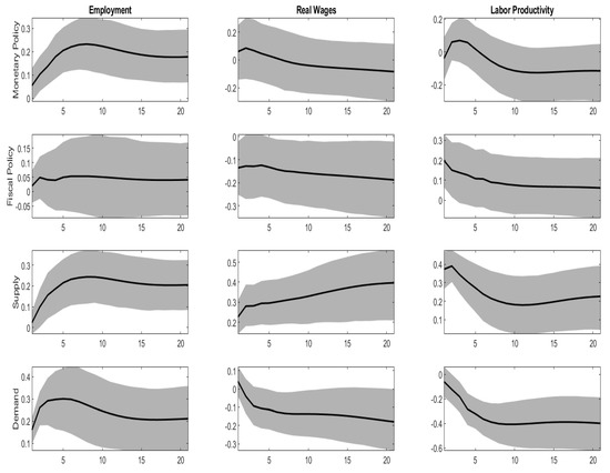
Figure 6.
Impulse-response functions. Solid line point estimate, gray areas 68% confidence bands.
The finding above is consistent with a stream of empirical and theoretical work concerning the interactions between growth and cycle. Empirical evidence of a long-run negative effect of a positive demand shock on productivity is reported in Bean (1990), Saint-Paul (1993), and Galí and and Hammour (1992), where an impulse response function almost identical to the one obtained here is found by using a structural VAR approach. Possible explanations are provided by theoretical works which, in various ways, revive the Schumpeterian view of recessions as providing a cleansing mechanism for reducing organizational inefficiencies and resource misallocations. During recessions, less efficient firms become unprofitable and shut down, thus improving average productivity (Caballero and Hammour 1994). Moreover, the opportunity cost of undertaking productivity-enhancing activities are lower, so that recessions are the right time to reorganize production, and/or improve the matching between workers and firms, implement new technologies, invest in human capital (Davis and Haltiwanger 1992; Hall 1991; Aghion and Saint-Paul 1998). Such efficiency effects are long-lasting.11
The above finding has a relevant implication for the empirical research. A widespread practice in structural VAR literature is to identify technology shocks as the only ones having long-run effects on productivity (Galí 1999; Christiano et al. 2004). However, if demand also affects productivity, this identification assumption may produce a mixture of true positive technology shocks and negative demand shocks, leading to incorrect conclusions. For instance, the finding that technology reduces hours worked (Galí 1999) could be due to the negative demand component. Indeed, our supply shock have a significant positive impact on hours worked (not shown). Moreover, the puzzling finding that technology has little effect on investment (Christiano et al. 2004) may result from positive technology effects canceling out with negative demand effects. Actually with our identification procedure supply shocks account for about 45% of fluctuations in investment at the 6-year horizon (see Table 2).
4.5. Policy Implications
From the previous results we draw a few policy implications. First, policy matter. Indeed both fiscal and monetary policy have sizable effects on output, employment and other real economic activity variables. Monetary policy appear to be very important for price fluctuations explaining around one third of the variance of GDP deflator inflation. On the contrary, fiscal policy seems to play a more limited role for prices.
Second, the evidence suggests a strong countercyclical systematic response of both monetary and fiscal authorities to non-policy demand shocks. Given that discretionary policy has sizable effects on both output and prices, systematic policy could be effective in controlling inflation and reducing output fluctuations arising from non-policy demand. As a consequence, output fluctuations originated by non-policy demand, which, as documented above, are fairly small in comparison with supply-driven variations, could be much larger if systematic policy where not in place. Unfortunately, with the present model we cannot proceed to evaluate the quantitative importance of stabilization policies, nor we can say whether the corresponding variance reduction over-compensates for discretionary policies, which, as we have seen, are non-negligible sources of additional fluctuations.
Third, systematic counter-cyclical policies, if successful in reducing fluctuation, may have long-run ’side effects’. Specifically, expansive measures following negative demand shocks, while not hurting GDP growth, may permanently support employment on one hand, and reduce per capita GDP and real wages, on the other hand. On balance, such effects are not necessarily undesirable. However, policy makers should be fully aware of the efficiency issues related to public support for employment and shaky companies, in order to design intervention properly.
5. Conclusions
This paper studies the sources of business cycle fluctuations and the role of macroeconomic policies using a structural factor model. Our main results are the following.
First, theories based on the existence of a single source of fluctuations as well as theories relying on a large number of shocks are inconsistent with our evidence. The US economy can be well described by a number of shocks between 2 and 5.
Second, by specifying a four-shock model we find that both demand and supply components are important to explain fluctuations in real macroeconomic variables, although the relative importance varies, depending on the specific variable considered. Supply explains most of GDP volatility while demand prevails for employment and other labor market variables. Fluctuations in prices are mostly explained by demand shocks.
Third, policy is important. Discretionary policies produce sizable effects on output and prices, with little evidence of crowding out effects of public expenditure. Both fiscal and monetary authorities follow systematic policy rules reacting mainly to private demand shocks. Such stabilization policies could in principle be very effective in reducing demand driven fluctuations.
Finally, non-policy demand shocks, while being long run neutral on GDP, have a large and permanent negative effect on productivity. Such a result is consistent with the Schumpeterian view of crises as providing a “cleansing” device for reducing inefficiencies and resource misallocations.
Author Contributions
Conceptualization: L.G. and M.F.; methodology: M.F.; software: L.G.; formal analysis: M.F.; data curation: L.G.; writing—original draft: L.G. and M.F.; writing—review and editing: L.G.; visualization: L.G.; supervision: M.F and L.G.; funding acquisition: L.G. and M.F. All authors have read and agreed to the published version of the manuscript.
Funding
This research was funded by the Italian Ministry of Research and University, PRIN 2017, grant J44I20000180001, the Spanish Ministry of Science and Innovation, through the Severo Ochoa Programme for Centres of Excellence in R&D (CEX2019-000915-S), the Spanish Ministry of Science, Innovation and Universities through grant PGC2018-094364-B-I00.
Data Availability Statement
The data presented in this study are available on request from the corresponding author. The data are not publicly available since some series was taken from Data Stream and several publicly available series were transformed by the authors (see Section 3.1 and Appendix A for details).
Conflicts of Interest
The authors declare no conflict of interest. The funders had no role in the design of the study; in the collection, analyses, or interpretation of data; in the writing of the manuscript, or in the decision to publish the results.
Appendix A. Data
Transformations: 1 = levels, 2 = first differences of the original series, 5 = first differences of logs of the original series.
| No. Series | Transf. | Mnemonic | Long Label |
| 1 | 5 | GDPC1 | Real Gross Domestic Product, 1 Decimal |
| 2 | 5 | GNPC96 | Real Gross National Product |
| 3 | 5 | NICUR/GDPDEF | National Income/GDPDEF |
| 4 | 5 | DPIC96 | Real Disposable Personal Income |
| 5 | 5 | OUTNFB | Nonfarm Business Sector: Output |
| 6 | 5 | FINSLC1 | Real Final Sales of Domestic Product, 1 Decimal |
| 7 | 5 | FPIC1 | Real Private Fixed Investment, 1 Decimal |
| 8 | 5 | PRFIC1 | Real Private Residential Fixed Investment, 1 Decimal |
| 9 | 5 | PNFIC1 | Real Private Nonresidential Fixed Investment, 1 Decimal |
| 10 | 5 | GPDIC1 | Real Gross Private Domestic Investment, 1 Decimal |
| 11 | 5 | PCECC96 | Real Personal Consumption Expenditures |
| 12 | 5 | PCNDGC96 | Real Personal Consumption Expenditures: Nondurable Goods |
| 13 | 5 | PCDGCC96 | Real Personal Consumption Expenditures: Durable Goods |
| 14 | 5 | PCESVC96 | Real Personal Consumption Expenditures: Services |
| 15 | 5 | GPSAVE/GDPDEF | Gross Private Saving/GDP Deflator |
| 16 | 5 | FGCEC1 | Real Federal Consumption Expenditures & Gross Investment, 1 Decimal |
| 17 | 5 | FGEXPND/GDPDEF | Federal Government: Current Expenditures/GDP deflator |
| 18 | 5 | FGRECPT/GDPDEF | Federal Government Current Receipts/GDP deflator |
| 19 | 2 | FGDEF | Federal Real Expend-Real Receipts |
| 20 | 1 | CBIC1 | Real Change in Private Inventories, 1 Decimal |
| 21 | 5 | EXPGSC1 | Real Exports of Goods & Services, 1 Decimal |
| 22 | 5 | IMPGSC1 | Real Imports of Goods & Services, 1 Decimal |
| 23 | 5 | CP/GDPDEF | Corporate Profits After Tax/GDP deflator |
| 24 | 5 | NFCPATAX/GDPDEF | Nonfinancial Corporate Business: Profits After Tax/GDP deflator |
| 25 | 5 | CNCF/GDPDEF | Corporate Net Cash Flow/GDP deflator |
| 26 | 5 | DIVIDEND/GDPDEF | Net Corporate Dividends/GDP deflator |
| 27 | 5 | HOANBS | Nonfarm Business Sector: Hours of All Persons |
| 28 | 5 | OPHNFB | Nonfarm Business Sector: Output Per Hour of All Persons |
| 29 | 5 | UNLPNBS | Nonfarm Business Sector: Unit Nonlabor Payments |
| 30 | 5 | ULCNFB | Nonfarm Business Sector: Unit Labor Cost |
| 31 | 5 | WASCUR/CPI | Compensation of Employees: Wages & Salary Accruals/CPI |
| 32 | 5 | COMPNFB | Nonfarm Business Sector: Compensation Per Hour |
| 33 | 5 | COMPRNFB | Nonfarm Business Sector: Real Compensation Per Hour |
| 34 | 5 | GDPCTPI | Gross Domestic Product: Chain-type Price Index |
| 35 | 5 | GNPCTPI | Gross National Product: Chain-type Price Index |
| 36 | 5 | GDPDEF | Gross Domestic Product: Implicit Price Deflator |
| 37 | 5 | GNPDEF | Gross National Product: Implicit Price Deflator |
| 38 | 5 | INDPRO | Industrial Production Index |
| 39 | 5 | IPBUSEQ | Industrial Production: Business Equipment |
| 40 | 5 | IPCONGD | Industrial Production: Consumer Goods |
| 41 | 5 | IPDCONGD | Industrial Production: Durable Consumer Goods |
| 42 | 5 | IPFINAL | Industrial Production: Final Products (Market Group) |
| 43 | 5 | IPMAT | Industrial Production: Materials |
| 44 | 5 | IPNCONGD | Industrial Production: Nondurable Consumer Goods |
| 45 | 1 | AWHMAN | Average Weekly Hours: Manufacturing |
| 46 | 2 | AWOTMAN | Average Weekly Hours: Overtime: Manufacturing |
| 47 | 2 | CIVPART | Civilian Participation Rate |
| 48 | 5 | CLF16OV | Civilian Labor Force |
| 49 | 5 | CE16OV | Civilian Employment |
| 50 | 5 | USPRIV | All Employees: Total Private Industries |
| 51 | 5 | USGOOD | All Employees: Goods-Producing Industries |
| 52 | 5 | SRVPRD | All Employees: Service-Providing Industries |
| 53 | 5 | UNEMPLOY | Unemployed |
| 54 | 5 | UEMPMEAN | Average (Mean) Duration of Unemployment |
| 55 | 1 | UNRATE | Civilian Unemployment Rate |
| 56 | 5 | HOUST | Housing Starts: Total: New Privately Owned Housing Units Started |
| 57 | 1 | FEDFUNDS | Effective Federal Funds Rate |
| 58 | 1 | TB3MS | 3-Month Treasury Bill: Secondary Market Rate |
| 59 | 1 | GS1 | 1-Year Treasury Constant Maturity Rate |
| 60 | 1 | GS10 | 10-Year Treasury Constant Maturity Rate |
| 61 | 1 | AAA | Moody’s Seasoned Aaa Corporate Bond Yield |
| 62 | 1 | BAA | Moody’s Seasoned Baa Corporate Bond Yield |
| 63 | 1 | MPRIME | Bank Prime Loan Rate |
| 64 | 5 | BOGNONBR | Non-Borrowed Reserves of Depository Institutions |
| 65 | 5 | TRARR | Board of Governors Total Reserves, Adjusted for Changes in Reserve |
| 66 | 5 | BOGAMBSL | Board of Governors Monetary Base, Adjusted for Changes in Reserve |
| 67 | 5 | M1SL | M1 Money Stock |
| 68 | 5 | M2MSL | M2 Minus |
| 69 | 5 | M2SL | M2 Money Stock |
| 70 | 5 | BUSLOANS | Commercial and Industrial Loans at All Commercial Banks |
| 71 | 5 | CONSUMER | Consumer (Individual) Loans at All Commercial Banks |
| 72 | 5 | LOANINV | Total Loans and Investments at All Commercial Banks |
| 73 | 5 | REALLN | Real Estate Loans at All Commercial Banks |
| 74 | 5 | TOTALSL | Total Consumer Credit Outstanding |
| 75 | 5 | CPIAUCSL | Consumer Price Index For All Urban Consumers: All Items |
| 76 | 5 | CPIULFSL | Consumer Price Index for All Urban Consumers: All Items Less Food |
| 77 | 5 | CPILEGSL | Consumer Price Index for All Urban Consumers: All Items Less Energy |
| 78 | 5 | CPILFESL | Consumer Price Index for All Urban Consumers: All Items Less Food & Energy |
| 79 | 5 | CPIENGSL | Consumer Price Index for All Urban Consumers: Energy |
| 80 | 5 | CPIUFDSL | Consumer Price Index for All Urban Consumers: Food |
| 81 | 5 | PPICPE | Producer Price Index Finished Goods: Capital Equipment |
| 82 | 5 | PPICRM | Producer Price Index: Crude Materials for Further Processing |
| 83 | 5 | PPIFCG | Producer Price Index: Finished Consumer Goods |
| 84 | 5 | PPIFGS | Producer Price Index: Finished Goods |
| 85 | 5 | OILPRICE | Spot Oil Price: West Texas Intermediate |
| 86 | 5 | USSHRPRCF | US Dow Jones Industrials Share Price Index (EP) NADJ |
| 87 | 5 | US500STK | US Standard & Poor’s Index if 500 Common Stocks |
| 88 | 5 | USI62...F | US Share Price Index NADJ |
| 89 | 5 | USNOIDN.D | US Manufacturers New Orders for Non Defense Capital Goods (BCI 27) |
| 90 | 5 | USCNORCGD | US New Orders of Consumer Goods & Materials (BCI 8) CONA |
| 91 | 1 | USNAPMNO | US ISM Manufacturers Survey: New Orders Index SADJ |
| 92 | 5 | USVACTOTO | US Index of Help Wanted Advertising VOLA |
| 93 | 5 | USCYLEAD | US The Conference Board Leading Economic Indicators Index SADJ |
| 94 | 5 | USECRIWLH | US Economic Cycle Research Institute Weekly Leading Index |
| 95 | 5 | GS10-FEDFUNDS | |
| 96 | 5 | GS1-FEDFUNDS | |
| 97 | 5 | BAA-FEDFUNDS | |
| 98 | 5 | GEXPND/GDPDEF | Government Current Expenditures/GDP deflator |
| 99 | 5 | GRECPT/GDPDEF | Government Current Receipts/GDP deflator |
| 100 | 1 | GDEF | Governnent Real Expend-Real Receipts |
| 101 | 5 | GCEC1 | Real Government Consumption Expenditures & Gross Investment, 1 Decimal |
| 102 | 1 | GS5 | 5-Year Treasury Constant Maturity Rate |
Notes
| 1 | An alternative approach is represented by Banbura et al. (2010), which develops a Bayesian VAR model that can handle many economic time series. |
| 2 | Observe that, if , the residuals of the above VAR relation have a singular variance covariance matrix. Equations (1) to (3) need further qualification to ensure that all of the factors are loaded, so to speak, by enough variables with large enough loadings (see FGLR, Assumption 4); this “pervasiveness” condition is necessary to have uniqueness of the common and the idiosyncratic components, as well as the number of static factors r and dynamic factors q. |
| 3 | Unlike the dynamic factors, the static factors do not have a structural economic interpretation; rather, they are a statistical tool which is useful to model the dynamics of the system. Loosely speaking, given the number of primitive shocks q, the number of “static factors” r governs the “degree of heterogeneity” of the impulse–response functions. For instance, in the simple case , if all the impulse–response functions are proportional. On the other hand, if r is larger, different variables can load the shock with different delays, so that we may have leading, coincident and lagging variables. If r is large enough, any (finite order) MA dynamics can be written in the form (1)–(3) (FGLR, Section 2). |
| 4 | Note that has to be large enough to retain relevant lagged auto- and cross-covariances. |
| 5 | We impose an upper bound to the number of impulse–response functions to retain for each step of the bootstrap procedure in order to avoid that a single bootstrap provide a disproportionately large number of functions. |
| 6 | Outliers were detected as values differing from the median more than 6 times the interquartile difference and replaced with the median of the five previous observations. |
| 7 | The test has two parameters identifying the lower and the upper bound of the frequencies of interest. Since we are mainly interested in business cycle fluctuations, we set such parameters in such a way to include waves of periodicity between 2 and 12 years. |
| 8 | The Bai and Ng criteria have two parameters. We set for all criteria and , , , . Such values produced good results in our simulations (not shown here). |
| 9 | The real federal deficit is constructed as the difference between current federal expenditures and current federal receipts, divided by the GDP deflator. |
| 10 | For the monetary policy shock a similar picture emerges but the effect on labor productivity is not significant. |
| 11 | According to the above explanations, productivity is related to the business cycle, rather than demand per se). This is consistent with our estimated response of productivity to supply shocks, which reaches its maximum after about one year and then declines sharply, dissipating about one half of the impact effect in the following six quarters (see Figure 6). |
References
- Aghion, Philippe, and Gilles Saint-Paul. 1998. Virtues of Bad Times: Interaction between Productivity Growth and Economic Fluctuations. Macroeconomic Dynamics 2: 322–44. [Google Scholar] [CrossRef]
- Altissimo, Filippo, Riccardo Cristadoro, Mario Forni, Marco Lippi, and Giovanni Veronese. 2010. New EuroCOIN: Tracking Economic Growth in Real Time. The Review of Economics and Statistics 92: 1024–34. [Google Scholar] [CrossRef]
- Alessi, Lucia, and Mark Kerssenfischer. 2019. The response of asset prices to monetary policy shocks: Stronger than thought. Journal of Applied Econometrics 34: 661–72. [Google Scholar] [CrossRef]
- Altug, Sumru. 1989. Time-to-Build and Aggregate Fluctuations: Some New Evidence. International Economic Review 30: 889–920. [Google Scholar] [CrossRef] [Green Version]
- Amengual, Dante, and Mark W. Watson. 2007. Consistent Estimation of the Number of Dynamic Factors in a Large N and T Panel. Journal of Business and Economic Statistics 25: 91–96. [Google Scholar] [CrossRef]
- Bai, Jushan. 2003. Inferential Theory for Factor Models of Large Dimensions. Econometrica 71: 135–71. [Google Scholar] [CrossRef]
- Bai, Jushan, and Serena Ng. 2002. Determining the number of factors in approximate factor models. Econometrica 70: 191–221. [Google Scholar] [CrossRef] [Green Version]
- Bai, Jushan, and Serena Ng. 2007. Determining the Number of Primitive Shocks in Factor Models. Journal of Business and Economic Statistics 25: 52–60. [Google Scholar] [CrossRef] [Green Version]
- Banbura, Marta, Domenico Giannone, and Lucrezia Reichlin. 2010. Large Bayesian vector auto regressions. Journal of Applied Econometrics 25: 71–92. [Google Scholar] [CrossRef]
- Bean, Charles R. 1990. Endogenous growth and the pro-cyclical behaviour of productivity. European Economic Review 34: 355–63. [Google Scholar] [CrossRef]
- Bernanke, Ben, and Jean Boivin. 2003. Monetary policy in a data-rich environment. Journal of Monetary Economics 50: 525–46. [Google Scholar] [CrossRef] [Green Version]
- Bernanke, Ben S., Jean Boivin, and Piotr Eliasz. 2005. Measuring Monetary Policy: A Factor Augmented Autoregressive (FAVAR) Approach. Quarterly Journal of Economics 120: 387–422. [Google Scholar]
- Blanchard, Olivier Jean, and Danny Quah. 1989. The Dynamic Effects of Aggregate Demand and Supply Disturbances. American Economic Review 79: 655–73. [Google Scholar]
- Blanchard, Olivier Jean, and Roberto Perotti. 2002. An Empirical Characterization of the Dynamic Effects of Changes in Government Spending and Taxes on Output. Quarterly Journal of Economics 117: 1329–68. [Google Scholar] [CrossRef] [Green Version]
- Caballero, Ricardo, and Mohamad L. Hammour. 1994. The Cleansing Effect of Recessions. American Economic Review 84: 1350–68. [Google Scholar]
- Chamberlain, Gary. 1983. Funds, factors, and diversification in arbitrage pricing models. Econometrica 51: 1281–304. [Google Scholar] [CrossRef] [Green Version]
- Chamberlain, Gary, and Michael Rothschild. 1983. Arbitrage, factor structure and mean variance analysis in large asset markets. Econometrica 51: 1305–24. [Google Scholar] [CrossRef]
- Christiano, Lawrence J., Martin Eichenbaum, and Charles L. Evans. 1999. Monetary policy shocks: What have we learned and to what end? In Handbook of Macroeconomics. Amsterdam: Elsevier, vol. 1, pp. 65–148. [Google Scholar]
- Christiano, Lawrence J., Martin Eichenbaum, and Robert Vigfusson. 2004. The Response of Hours to a Technology Shock: Evidence Based on Direct Measures of Technology. Journal of the European Economic Association 2: 381–95. [Google Scholar] [CrossRef] [Green Version]
- Connor, Gregory, and Robert A. Korajczyk. 1988. Risk and return in an equilibrium APT. Application of a new test methodology. Journal of Financial Economics 21: 255–89. [Google Scholar] [CrossRef]
- Davis, Steven, and John Haltiwanger. 1992. Gross Job Creation, Gross Job Destruction, and Employment Reallocation. The Quarterly Journal of Economics 107: 819–63. [Google Scholar] [CrossRef]
- Forni, Mario, and Luca Gambetti. 2010. The Dynamic Effects of Monetary Policy: A Structural Factor Model Approach. Journal of Monetary Economics 57: 203–13. [Google Scholar] [CrossRef]
- Forni, Mario, Domenico Giannone, Marco Lippi, and Lucrezia Reichlin. 2009. Opening the black box: Structural factor models with large cross-sections. Econometric Theory 25: 1319–47. [Google Scholar] [CrossRef] [Green Version]
- Forni, Mario, Marc Hallin, Marco Lippi, and Lucrezia Reichlin. 2000. The generalized dynamic factor model: Identification and estimation. The Review of Economics and Statistics 82: 540–54. [Google Scholar] [CrossRef]
- Forni, Mario, Marc Hallin, Marco Lippi, and Lucrezia Reichlin. 2005. The generalized factor model: One-sided estimation and forecasting. Journal of the American Statistical Association 100: 830–40. [Google Scholar] [CrossRef] [Green Version]
- Forni, Mario, and Marco Lippi. 2001. The generalized dynamic factor model: Representation theory. Econometric Theory 17: 1113–41. [Google Scholar] [CrossRef] [Green Version]
- Galí, Jordi. 1999. Technology, Employment, and the Business Cycle: Do Technology Shocks Explain Aggregate Fluctuations? American Economic Review 89: 249–71. [Google Scholar] [CrossRef] [Green Version]
- Galí, Jordi, and Mohamad Hammour. 1992. Long-Run Effects of Business Cycles Papers 92–26. Columbia: Graduate School of Business. [Google Scholar]
- Geweke, John. 1977. The dynamic factor analysis of economic time series. In Latent Variables in Socio-Economic Models. Amsterdam: North Holland. [Google Scholar]
- King, Robert, Charles Plosser, James Stock, and Mark Watson. 1991. Stochastic Trends and Economic Fluctuations. American Economic Review 81: 819–40. [Google Scholar]
- Hall, Robert E. 1991. Recessions as reorganizations. In NBER Macroeconomics Annual. Cambridge: NBER. [Google Scholar]
- Hallin, Marc, and Roman Liška. 2007. Determining the number of factors in the general dynamic factor model. Journal of the American Statistical Association 102: 603–17. [Google Scholar] [CrossRef]
- Ireland, Peter N. 2004. A method for taking models to the data. Journal of Economic Dynamics and Control 28: 1205–26. [Google Scholar] [CrossRef] [Green Version]
- Leeper, Eric, Todd Walker, and Shu-Chun Yang. 2013. Fiscal Foresight and Information Flows. Econometrica 81: 1115–45. [Google Scholar]
- Lippi, Marco, and Lucrezia Reichlin. 1994. VAR analysis, non fundamental representation, Blaschke matrices. Journal of Econometrics 63: 307–25. [Google Scholar] [CrossRef]
- Quah, Danny. 1990. Permanent and Transitory Movements in Labor Income: An Explanation for “Excess Smoothness” in Consumption. Journal of Political Economy 98: 449–75. [Google Scholar] [CrossRef] [Green Version]
- Ramey, Valery A. 2011. Identifying Government Spending Shocks: It’s All in the Timing. Quarterly Journal of Economics 126: 1–50. [Google Scholar] [CrossRef]
- Ramey, Valery A., and Matthew D. Shapiro. 1998. Costly Capital Reallocation and the Effects of Government Spending. Carnegie Rochester Conference on Public Policy 48: 145–94. [Google Scholar] [CrossRef] [Green Version]
- Saint-Paul, Gilles. 1993. Productivity growth and the structure of the business cycle. European Economic Review 37: 861–83. [Google Scholar] [CrossRef]
- Sargent, Thomas J. 1989. Two Models of Measurements and the Investment Accelerator. The Journal of Political Economy 97: 251–87. [Google Scholar] [CrossRef]
- Sargent, Thomas J., and Christopher A. Sims. 1977. Business cycle modeling without pretending to have too much a priori economic theory. In New Methods in Business Research. Minneapolis: Federal Reserve Bank of Minneapolis. [Google Scholar]
- Sims, Christopher A. 1980. Macroeconomics and Reality. Econometrica 48: 1–48. [Google Scholar] [CrossRef] [Green Version]
- Sims, Christopher A. 1992. Interpreting the Macroeconomic Time Series Facts, The Effects of Monetary Policy. European Economic Review 36: 975–1011. [Google Scholar] [CrossRef]
- Smets, Frank, and Rafael Wouters. 2007. Shocks and Frictions in US Business Cycles: A Bayesian DSGE Approach. American Economic Review 97: 586–606. [Google Scholar] [CrossRef] [Green Version]
- Stock, James H., and Mark W. Watson. 2002a. Macroeconomic Forecasting Using Diffusion Indexes. Journal of Business and Economic Statistics 20: 147–62. [Google Scholar] [CrossRef] [Green Version]
- Stock, James H., and Mark W. Watson. 2002b. Forecasting Using Principal Components from a Large Number of Predictors. Journal of the American Statistical Association 97: 1167–79. [Google Scholar] [CrossRef] [Green Version]
- Stock, James H., and Mark W. Watson. 2005. Implications of Dynamic Factor Models for VAR Analysis. NBER Working Papers No. 11467. Cambridge: National Bureau of Economic Research, Inc. [Google Scholar]
- Uhlig, Harald. 2005. What are the effects of monetary policy on output? Results from an agnostic identification procedure. Journal of Monetary Economics 52: 381–419. [Google Scholar] [CrossRef] [Green Version]


Publisher’s Note: MDPI stays neutral with regard to jurisdictional claims in published maps and institutional affiliations. |
© 2021 by the authors. Licensee MDPI, Basel, Switzerland. This article is an open access article distributed under the terms and conditions of the Creative Commons Attribution (CC BY) license (https://creativecommons.org/licenses/by/4.0/).