Abstract
Interaction of fiscal and monetary policy is crucial for macroeconomic stability, especially for an economy with downward pressure as well as a tightened space for macro policy, like China. In this paper, we use a time-varying-parameter (TVP-VAR) model to study Chinese fiscal–monetary interaction and divide it into three periods. We claim that China went through a monetary dominant regime from 1996Q to 2017Q4 since the response of CPI to a fiscal expansion was negative in the short run and about zero in the long run, while the monetary expansion had positive effects on CPI. During this period, the response of government spending and money supply to each other’s shock had the same sign, indicating that the two policies acted as complements. However, we argue that 2008Q4 was a turning point that divided this period into two different periods. The response level of M2 growth rate to a fiscal expansion kept rising from 1996Q1 to 2008Q4, indicating the central bank’s increasingly active cooperation with fiscal policy, while it decreased from 2009Q1 to 2017Q4. Since 2018Q1, the economy has been going through a fiscal dominant regime in that the response of GDP growth rate and CPI to the fiscal expansion has sharply increased. We also argue that the relative change of the role between the two policies should be mainly attributed to the variation in the fiscal authority’s characteristics because fiscal response to a monetary shock has remained at a similar level the whole time, even if there have been changes in the characteristics of the central bank.
1. Introduction
Fiscal and monetary policies have long been the main policy instruments for stabilizing the macroeconomy. However, the 2008 Global Financial Crisis depressed economic development all over the world and made it hard for a single policy to realize recovery or stabilization because policy space has been compressed by the recession. For example, the US was facing a ‘Zero Lower Bond’ after the crisis. Thus, coordination of macro policies has become more necessary (Blanchard et al. 2010) and people have deepened concerns about the significance of policies’ interactions. In recent years, government debt to GDP ratio in China has been increasing, and the interest rate has been falling, indicating that the space to apply stabilization policies is not as sufficient as before. Hence, interaction between Chinese fiscal and monetary policy should be given more attention.
Being the largest emerging country in the world, China is different from other developed countries in many aspects such as population, marketization and so on and macro policies’ interactions in China may have their own mechanisms or characteristics. Moreover, the characteristics of fiscal–monetary interaction may not be constant over time. Cogley and Sargent (2005) point out that interior structural changes would happen in an economy. In fact, fiscal–monetary interaction in China might have undergone changes because both fiscal and monetary policy have been reformed and the preferences or characteristics of the authorities have varied over time. According to Guo and Li (2021), fiscal policy in China has experienced several transformations and they are strongly correlated with economic development. Yi (2009) reviews the interest rate marketization in China, asserting that the central bank keeps improving regulation methods in this process. China has experienced rapid development in fields like technology, education, poverty-reduction, etc. All of these elements would potentially change the characteristics of the interaction between macro policies. Hence it is reasonable to believe that the way in which fiscal and monetary policy interact with each other has gone through changes in these years.
In this paper, we aim to find out the aforementioned features, so we use a TVP-VAR model to examine the characteristics of fiscal–monetary interaction in China. Figures of time-varying impulse responses to fiscal and monetary shocks are given to show how fiscal and monetary policy affect the Chinese economy as well as their interactions. We divide the fiscal–monetary interaction into three periods, 1996Q1 to 2008Q4, 2009Q1 to 2017Q4 and 2018Q1 to 2020Q3. During these periods characteristics of the interaction are quite different.
We claim that 1996Q1 to 2017Q4 represents a monetary dominant (MD) regime since the response of CPI is negative to a fiscal expansion in the short run and about zero in the long run, while the monetary expansion has a positive effect on both GDP and CPI. During this period, the monetary and fiscal policy’s responses to each other’s shock are positive, implying that they act as complements. However, we argue that 2008Q4 is a turning point. The M2 response to the fiscal expansion keeps increasing from 1996Q1 to 2008Q4, showing the central bank’s increasingly active cooperation with fiscal policy, while the response level decreases from 2009Q1 to 2017Q4, though remaining at a relatively high level. This indicates the central bank’s effort to enhance its role after the 2008 crisis, but it is forced to cooperate with fiscal sides because of the high debt and leverage induced by the intensive fiscal policies after the recession. We also find that since 2018Q1, China is going through a fiscal-dominant regime because the effects that fiscal expansion have on GDP and CPI are positive. Moreover, compared with the MD regime before, the fiscal effects under an FD regime are much stronger.
In addition, we find that the response of government spending to a monetary expansion does not undergo a huge change during the whole sample period from 1996Q1 to 2020Q2, implying that, even if there have been changes in the role or channel of monetary policy, the fiscal authority always operates in its own way. In other words, the fiscal policy may ignore the monetary policy. We conclude that changes in the relative role between monetary and fiscal policy should be mainly attributed to the variation of the fiscal authority’s (government) characteristics or preferences. Also, we recommend that the fiscal policy should give more concern to monetary policy and both policies should pay more attention to the debt and macro leverage. Moreover, fiscal expansion alone will not be enough for long term growth and more concern should be given to the fiscal–monetary interaction.
In fact, the fiscal–monetary interaction is so important and there already have been some pieces of literature discussing about it, especially from a theoretical aspect, though they do not reach a consensus. Sargent and Wallace (1981) put forward a monetarist arithmetic. By applying transversality to the government’s (fiscal authority) present value budget constraint (PVBC), they obtained , where the three terms, respectively, refer to the inherited government debt, the central bank’s collection of seigniorage, government surpluses. Thus, they described the interaction between monetary and fiscal policy as a non-cooperative game. If the central bank gains the initiative and sets the path of inflation, then is determined; the government must set the path of surpluses to maintain PVBC. Similarly, if the government goes first, the central bank is forced to set inflation to maintain PVBC. Woodford (1996) claims that seigniorage is just a small part of revenue in developed countries; thus, the mechanism above remains to be discussed. Meanwhile, the fiscal theory of the price level (FTPL) that developed since the 1990s provides us with another perspective to understand the interaction between monetary and fiscal policy. FTPL, being different from the monetarist arithmetic, takes the government bonds as a nominal variable; thus, the PVBC can be written as:
The basic idea of FTPL is that only with a suitable coordination of monetary and fiscal policies can we obtain an equilibrium. According to Woodford (1995) and Canzoneri et al. (2001), when considering budget constraints, if primary surpluses are determined independently of the debt, the path of monetary policy and price must satisfy the PVBC; this can be called a fiscal dominant (FD) or non-Ricardian regime for the false Ricardian equivalence. If monetary policy and prices are determined by the supply and demand for money, and primary surpluses satisfy the PVBC, it can be called a monetary dominant (MD) or Ricardian regime. Leeper (1991) defines active policy as paying no attention to the state of government debt and being free to set its variable. He proved that a unique saddle path exists in either active monetary policy (AM) combined with passive fiscal policy (PF), similar to MD, or AF combined with PM, which is similar to FD.
While FTPL provides us with a new aspect to consider the monetary and fiscal policy’s interaction and coordination, criticisms towards FTPL have also emerged. Buiter (2002) argues that PVBC is a real constraint which government must follows and otherwise is invalid. Canzoneri et al. (2010) point out a coordination problem: How do the central bank and government know which policy regime or state to switch to? Davig et al. (2006) and Davig and Leeper (2011) allow for the random switching of monetary and fiscal policy between active and passive. They combine a regime-switching process with a DSGE model. In their work in 2006, despite there being periods with PM/PF and AM/AF, they find an equilibrium. In short, the theories of interaction between monetary and fiscal policy, or the policy trade-off as discussed in Bianchi and Melosi (2017), are inconclusive.
Besides theoretical discussions above, some empirical papers also study the interaction between fiscal and monetary policy. Muscatelli et al. (2004) suggest that the fiscal–monetary interactions are not consistent over time by applying a NK model. Fragetta and Kirsanova (2007) find that the model of fiscal dominance fits the UK better than Sweden. Reade (2011) emphasises the importance of fiscal–monetary policy interactions for the US after the 2008 recession. Gornemann et al. (2012) match their DSGE model to the American economy and make an interest rate shock to observe its effect. Zhang and Jin (2011) used the MS-VAR model to figure out the structural change of fiscal policy and monetary policy from 1980 to 2009. Cogley and Sargent (2005) demonstrate that autoregressive coefficients of VARs could evolve systematically over time and then they introduce the time-varying-parameter VAR (TVP-VAR) model to solve the problem. Gerba and Hauzenberger (2013) use the TVP-VAR method with a sign restriction to investigate interactions of US fiscal and monetary policy and they point out that there are significant differences between the Volcker period and the Great Recession. As we have discussed before, characteristics of Chinese fiscal–monetary interactions might go through changes. Thus in this paper, we apply the TVP-VAR model to study the characteristics of Chinese fiscal–monetary interactions.
In terms of the main contributions to the current literature, first, being different from other literature that use traditional VAR methods, we apply the TVP-VAR model, which not only shows the time-varying effect of fiscal and monetary policy, but also, more importantly, helps us gain an insight into the characteristics of fiscal–monetary interaction. Second, the TVP-VAR method helps us explain the endogenous change of regime more intuitively. Third, the time range of our research stretches to 2020, including the time after Covid-19 broke out.
In Section 2, we introduce the TVP-VAR model that we apply in this paper. The results of the model are discussed in Section 3. Based on time-varying impulse response figure, we analyze changes of the effect of a fiscal policy shock and monetary policy shock, respectively, in Section 3.1 and Section 3.2, as well as the characteristics of fiscal–monetary interaction. In Section 3.3, we extend our discussion of the interaction, researching some turning points of the time-varying response in detail. Section 4 is conclusions.
2. The TVP-VAR Model
To make a brief introduction to the TVP-VAR model, firstly we consider a structural VAR model:
where is a vector consisting of the variables we observed and are coefficient matrices. represents a structural shock which follows .
Moreover, we adopt the recursive identification, meaning that A is lower triangular.
Then the structural-form VAR can be written as a reduced-form VAR:
Define vector where is formed by stacking the elements in the rows of , and , where ⨂ denotes the Kronecker product. Thus we obtain:
Allowing parameters in Equation (2) to be time-variant, we can write the TVP-VAR model with stochastic volatility:
Following Nakajima (2011), we stack the elements of to form
Set where for and . To reduce the parameters that need to be estimated, we assume that:
where ,,.
Nakajima (2011) pointed out that whether or not take the diagonal assumption has no significant influence on empirical results, so we take them as diagonal matrices.The TVP-VAR is estimated based on Bayesian inference and the MCMC sampling method. The core idea is to sample the conditional posterior distribution recursively based on the most recent values of the conditioning parameters. We do not list more details about the algorithm here and a more specific procedure can be seen in Nakajima (2011).
3. Empirical Results and Discussion
Five Chinese macroeconomic variables at quarterly frequency included in our TVP-VAR model are growth rate of government spending, growth rate of money supply M2, nominal interest rate which is represented by a seven-day CHIBOR, the growth rate of nominal GDP and CPI, from 1996Q1 to 2020Q3. Quarterly CHIBOR is the weighted average of the monthly CHIBOR based on its trading volume. All of the variables reject the hypothesis of having a unit root, which can be seen in Table 1, so we can take them as stationary series.

Table 1.
Results of unit root test.
To estimate the model, we let MCMC sample 20,000 times and discard the 4000 samples in the burn-in period. According to Table 2, the posterior mean of the parameters all drop in the 95 percent credible intervals. The ’Geweke’ column is the CD statistic value, proposed by Geweke (1992), which shows the convergence of the Markov chain, and can be calculated by:
where is the i-th draw and is the standard deviation of for . Its distribution converges to a standard normal when MCMC sampling is a stationary series. The ’Inef’ column shows the value of the inefficiency factor, which is calculated by (Chib et al. 2002):
where is the sample autocorrelation at lag s. We set , . The values in the last two columns show that only one parameter rejects the hypothesis of convergence to the posterior distribution and only one inefficiency factor larger than 100 (just 102.7), indicating that the MCMC procedure, is credible.
Table 2.
TVP-VAR estimation results.
Being different from a typical VAR model, the impulse response of the TVP-VAR model can be drawn in a new dimension, where responses are computed at all points during the sample period, and we can treat it as a time-varying response, representing the (perhaps heterogeneous) responses to the same shock at different times. Specifically, we draw two-quarter, one-year and two-year ahead responses, separately. Our analysis mainly relies on these time-varying responses since we can gain an insight into the time-variant reaction of the variable to an exogenous shock.
3.1. Government Spending Shock
Figure 1 shows the time-varying impulse responses to a positive government shock or fiscal expansion. In terms of GDP growth rate, we find that since 2018Q1, both the two-quarter and one-year ahead response increase sharply from about 0.4 to 2.5 and 1.5, respectively, which is quite different from its previous reaction. At about the same time (2018Q2), the response of CPI turns from negative to positive and continues to increase, which is also radically different from its response before. Combining the two features, we argue that fiscal policy, since 2018Q1, begins to play a role in stimulating short-term economic by expanding the aggregate demand; we have seen a positive and sharply increasing response of CPI as well as GDP growth rate. Meanwhile, the response level of M2 growth rate to a government spending shock has gone through a huge decline since 2018Q1 and turned from positive to negative at about 2019Q4.
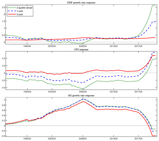
Figure 1.
Response to a Positive Government Spending Shock.
When a fiscal expansion happens, according to the FTPL theory, under an FD regime, either the central bank will increase the money supply to raise the seigniorage for PVBC, which is inconsistent with our finding that the level of M2 response decreases and its sign has changed, or the fiscal policy will show its wealthy effect and the GDP as well as the price level increases, which is similar to our finding after 2018Q1. The fiscal authority has made up its mind to enhance the dominance of fiscal policy since 2018Q1 and we assert that the economy is going through a fiscal dominant (FD) regime. What is more, although this pattern seems to be desirable in the short run, we keep in mind that fiscal expansion alone will not be enough for long term growth because the two-year ahead response shows that the relative long-run GDP growth rate is stationary, with a level of about 0.25 for the whole sample period. We also emphasise that the FD regime does not mean the absence of monetary policy. The large decline of the response level of M2 growth rate to government spending shock since 2018Q1 and the change of its sign (even in the long run, as the red line shows) show the central bank’s effort to avoid an increasing debt since the central bank will not support the deficits by simply issuing money. For example, at about the middle of the year 2020, the Chinese central bank clearly stated that it will not support the monetization of fiscal deficits.
To be more intuitive, compare the responses to the government spending shock from 1996Q1 to 2017Q4 with responses from 2018Q1 to 2020Q3. The response of CPI remains negative in the short run, reaching its bottom at 2008Q4, and stays at about zero in the long run, which is not consistent with FTPL’s definition of the FD regime. Thus, we conclude this period as a monetary dominant (MD) regime. In fact, the effect of monetary expansion on GDP and CPI (a positive response of GDP and CPI) also confirms our claim, which we will put forward in Section 3.2. In addition, while the negative response of CPI to fiscal shock is not in line with traditional economic theory, some studies indeed have found similar results, for example, Canova and Pappa (2007), Mountford and Uhlig (2009). A potential explanation for the negative short-run response of CPI to a fiscal expansion is the imperfect substitutability of private and public sector investment. For example, public investment may offer cheaper housing than the private sector and thus CPI falls. Moreover, the Chinese government lays emphasis on infrastructure investment, expecting to improve the economic structure and distribution of goods, which may show its effects on GDP in the long run and lead to the price level not increasing currently. The positive sign of the two-year ahead response of GDP growth rate provides the evidence for this idea. What is more, the effect of fiscal policy under the MD regime, whether in terms of GDP of CPI, may not be satisfactory when compared with its effect under the FD regime.
However, we find that 2008Q4 is a turning point since the response level of the M2 growth rate kept rising from 1996Q1 to 2008Q4, indicating its increasingly active cooperation with the fiscal side, while it has decreased since 2009Q1, implying that the central bank enhanced its role after the crisis. In terms of the level of the M2 response, however, it kept at a relatively high level from 2009Q1 to 2017Q4, in contrast to the period after 2018Q1. In fact, for the pressure of intensive fiscal policy after the crisis, such as the Chinese ‘Four Trillion Fiscal Stimulus’, the M2 response, to some extent, was forced not to decline too dramatically and persistently to avoid default induced by the fiscal side. Moreover, recovery from recession requires the maintenance of liquidity in the market. Thus, the reaction of the central bank is key for economic stability during this period (2009Q1 to 2017Q4). Moreover, both the two-quarter and one-year ahead response level of GDP growth rate went through a decline from 1996Q1 to 2008Q4 and reached a bottom at 2008Q4, implying that the effect of government’s fiscal policy on the economy, at least in the short run, gradually declined in this period. The short-run GDP response increased right after 2008Q4, which implies the stimulus of fiscal expansion after the recession, however, at the cost of high leverage. The CPI response also increased right after 2008Q4, implying a short-term fiscal stimulus, while overall it remained negative, which is the reason we conclude this period as MD regime.
In addition, recently many researchers have considered how covid-19 affects the economy. From Figure 1, we find that there are turning points of the response level of GDP growth rate, CPI and M2 growth rate at 2020Q1, indicating the epidemic’s shock. However, the scale of change is not so large and the sign of the responses has not changed so far, which still indicates an FD regime.
3.2. Monetary Policy Shock
In Section 3.1, we divide the sample period into three parts, 1996Q1 to 2008Q4, 2009Q1 to 2017Q4 and 2018Q1 to 2020Q3, based on the response of CPI and the FTPL theory, as well as the response of macro variables. However, we have not analyzed the fiscal–monetary interaction in depth because the interaction refers to the reaction of fiscal and monetary policy to each other’s behavior. In this section, combining the response of fiscal side to a monetary shock with the analysis before, we try to gain an insight into the characteristics of the fiscal–monetary interaction and its evolution. However, firstly we analyse the effects of the monetary shock.
Figure 2 shows the time-varying impulse responses to a positive M2 growth rate shock. It turns out that the shock has a durable effect on GDP, with long term GDP growth rate response remaining over 0.26 during the sample period (as shown by the red line). When it comes to inflation (CPI), while it does not show an instant response to the M2 shock (because the two-quarter ahead response is quite near zero), the one-year ahead and two-year ahead response show that the shock’s effect on inflation is more obvious in the long run, around 0.15 during the sample period, as depicted by the blue-dashed line and the red line. Thus, we assert that monetary expansion has a more significant effect on CPI in the long run than in the short run, which can be described as a time-lag feature. Moreover, the response of GDP growth rate and CPI to a monetary expansion is consistent with our judgment in Section 3.1 that both 1996Q1 to 2008Q4 and 2009Q1 to 2017Q4 belong to an MD regime.
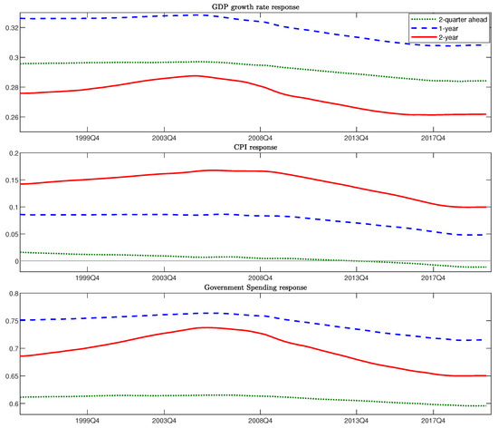
Figure 2.
Response to a Positive M2 Growth Rate Shock.
The responses of GDP growth rate and CPI, on the whole, do not go through a huge change through the sample period, which implies that the influence of money supply on the macroeconomy is stationary. This is quite intuitive because, according to the Chinese central bank report, the general principle of monetary policy is stabilized and it adjusts according to the market demand for liquidity, to avoid the huge volatility of GDP and CPI.
What are the characteristics of the fiscal–monetary interaction and what leads to changing it? The third figure in Figure 2 shows that the response of government spending to monetary expansion remained positive during the sample period. This indicates that, when it comes to a monetary shock, the government tends to have a similar reaction, a fiscal expansion. Recall that from 1996Q1 to 2017Q4, the response of M2 growth rate to a fiscal expansion remained positive, so we claim that during both periods, the fiscal and monetary policies acted as complements. Since 2018Q1, the response level of M2 to fiscal expansion has decreased sharply, indicating that the two policies’ complementarity is declining. After 2019Q4, the response of M2 turns from positive to negative and continues to decline, while the response of fiscal policy to a monetary shock remains positive, implying the asymmetry of the two policies. Moreover, the GDP response to a fiscal expansion hugely increases after 2018Q1, while keeps stationary concerning a monetary expansion, indicating that the fiscal–monetary interaction since 2018Q1 significantly promotes the effect of fiscal policy under the FD regime, especially compared with the two periods before when monetary policy cooperated with the fiscal side, whether actively or passively.
We also find that the response level of government spending is quite stationary during the sample period. This indicates that even if there have been changes in the role or characteristics of monetary policy, the government always operates in its own way, or ignores the central bank. Thus, we assert that the variation of the characteristics or preference of fiscal authority (for example, it has begun to take control since 2018Q1) should mainly accounts for the change of the relative role between fiscal and monetary policy. What is more, the covid-19 shock does not affect the effects of monetary policy significantly because the response level has not gone through obvious changes as is shown in Figure 2.
3.3. Further Discussion about the Turning Points
In previous sections, we claimed that the characteristics of the fiscal–monetary interaction has gone through changes during the sample period. Here, we are going to talk about more details. A new tool we use is the impulse response function at a given time; it is different from the time-varying response function in which shocks happen at every point and responses are given after a certain time period. Inversely, shocks happen at given time and responses are reported within a long time period. We use this new tool to analyze the evolution of a shock’s effect.
We choose four time points, 2005Q4, 2008Q4, 2010Q4 and 2020Q2, giving a shock at each time point to observe the path of the response. These time points are selected for their social backgrounds. In 2008, the Global Economic Crisis broke out. Since 2010, the Chinese government debt problem started to aggravate. In 2020, the covid-19 pandemic broke out and shocked the Chinese economy. On top of that, we chose 2005Q4 for comparison. Comparison between these time points can help us go deeped into understanding the characteristics of the different periods. Figure 3 depicts the response of M2 growth rate to a fiscal shock and the government spending response to a monetary supply shock.
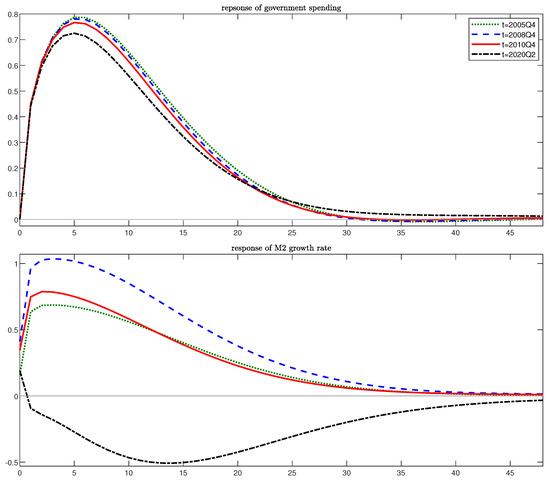
Figure 3.
Government Spending and M2 growth rate response to each other’s shock at a given time.
Figure 3 shows that not only the level, but also the evolution of the responses of government spending to a monetary expansion at different time points are close to each other, which corresponds with our finding that the reaction of fiscal authority (government) to a monetary shock is stationary during the sample period, implying the fiscal authority’s similar reaction to a monetary expansion. Specifically, all responses of government spending peak at the fifth quarter after the monetary shock and then gradually decline to zero. From this finding, we can draw the fact that monetary policy has a time-lag feature; its work usually gets to a maximum after a year.
M2 growth rate shows a relative medium level of positive responses to a government spending shock at 2005Q4 and 2010Q4. The response peaks after two quarters and then gradually declines to zero. The response to a fiscal shock given at 2008Q4 is higher than others until all of them converged to zero, confirming our previous conclusion that monetary policy’s cooperation with a fiscal policy were increasingly active before this time. Besides, around this time point, China was faced with large pressure induced by the global financial crisis. To avoid aggregate demand falling sharply, the Chinese government (fiscal side) poured four trillion yuan into the market alternately, which also needs the support of monetary policy.M2 response at 2020Q2, however, is very different from those at other time points. It turns to negative in the first quarter after the shock, decreasing to a bottom after the 14th quarter and finally converging to zero. This result colludes with the fact that the response of M2 to a government spending shock turns negative at about 2019Q4, even after a long time, implicitly showing that when there comes a positive fiscal shock, the central bank will not finance the government by issuing money. For one thing, it shows the enhancement of the role of the central bank. In fact, Chinese central has laid more emphasis on risk management and the role of monetary policy because of the recession and has realized that monetary policy should not focus on too many goals, such as financing the fiscal debt. Also, as is shown in Figure 1, the response of CPI to government spending shock surged and became positive at about 2018Q2 and continues to increase quickly, which can bring about inflation pressure under a fiscal expansion. Thus, the decline in the M2 growth rate is desirable since it avoids inducing higher inflation in the future. What is more, in 2020, housing prices in most Chinese cities go up at a distinctly faster pace, so the Chinese economy faces a trend of increasingly relying on real estate. To prevent more money from flowing into real estate, it is reasonable for the central bank to slow down the increase of money supply under a fiscal expansion.
In addition, another interesting thing we have pointed out in Section 3.1 is that, although the response of the M2 growth rate to a fiscal expansion declines in the period from 2009Q1 to 2017Q4, it remains at a relatively high level. We argue that the intensive action of fiscal policy limits the enhancement in the role of the central bank. For example, the ‘Four Trillion Stimulus’ added to the fiscal burden and the increasing macro leverage since 2010 in China forced the M2 response not to decrease dramatically, thus limiting the role of the central bank. We claim that during this period, the interaction of fiscal–monetary policy was undesirable since monetary policy was forced to keep pace with fiscal policy to some extent, accompanied by a growing leverage. However, since 2018Q1, the M2 response turned down again, rapidly. An explanation for this is that when the central bank always satisfies the fiscal side (for example, maintains PVBC), the government might continue to implement an expansion because the government believes that the monetary policy will react accordingly as it used to, which could induce an increasingly higher leverage rate. Thus, since 2018Q1, the central bank has strengthened its role and management of macro leverage. While the central bank’s reaction since 2018Q1 is different from its behavior before, the rapid increasing response of GDP and CPI shows that, under this pattern, fiscal policy turns out to be more effective in stimulating the economy. The reason is that the decline in the level of M2 response makes people believe the authority’s intention to control the high leverage. The transformation of people’s expectations smoothed the channel through which policy works; hence, the efficiency of the policy was enhanced. The improved efficiency, which the fiscal–monetary interaction brought about since 2018Q1 is important for China because the downward pressure is serious, especially after 2016.
4. Conclusions
In this paper, we use the TVP-VAR model to gain an insight into the characteristics of the Chinese fiscal–monetary policy interaction and the potential changes in it. One of the most crucial advantage of the TVP-VAR model is that it captures the time-varying feature of the parameters and the change of the interaction’s characteristics. Relying mainly on the time-varying impulse response function, this paper makes a comprehensive discussion of the Chinese fiscal–monetary policy interaction. By combining the time-varying response of fiscal and monetary policy to each other’s shock, as well as the responses of other macro variables, we divide the characteristics of the fiscal–monetary interaction into three periods, 1996Q1 to 2008Q4, 2009Q1 to 2017Q4 and 2018Q1 to 2020Q3.
We find that from 1996Q1 to 2017Q4, the response of CPI is negative to a fiscal expansion in the short run and about zero in the long run, while the monetary expansion has a positive effect on both GDP and CPI. Thus, we conclude this period to be a monetary dominant regime. Moreover, both the monetary and fiscal policies’ responses to each other’s shock are positive, implying that they act as complements. However, we argue that 2008Q4 is a turning point that divided this period into two different periods. From 1996Q1 to 2008Q4, the level of the monetary response to a fiscal expansion keeps rising, indicating the central bank’s increasingly active cooperation with fiscal authority. While from 2009Q1 to 2017Q4, the response level of the M2 growth rate goes through a decline, although still remaining at a relatively high level. This indicates that the central bank tried to enhance its role after the crisis, while to some extent it was still forced to cooperate with the fiscal side. Since 2018Q1, the economy has been going through a fiscal dominant regime (FD); the response of GDP and CPI to a fiscal expansion are positive and increasing sharply. During this period, the complementarity of fiscal and monetary policy has decreased and since about 2019Q4, the two policies have not acted as complements any more. In addition, the effect of fiscal expansion under the MD regime is significantly weaker than that under the FD regime. We also claim that variation in the fiscal authority’s characteristics should mainly account for the relative change of the role between fiscal and monetary policy because the fiscal response to a monetary shock is quite stationary during the whole sample period, regardless of the changes in the characteristics of the central bank.
Based on our findings, we put forward three recommendations for macro policy. First is that, for the effectiveness of macro policies, both fiscal and monetary authority should pay attention to the control of debt and macro leverage. This in turn requires the central bank to avoid issuing too much currency even if under a fiscal expansion, and the fiscal authority to avoid implementing fiscal expansion persistently only for short-run growth. Second is that fiscal decisions should give more concern to the action of the central bank. As we have pointed out, the fiscal response to a monetary shock is quite stationary during the sample period even if there have been changes in the characteristics of the central bank. This could be harmful for fiscal–monetary interaction and limits the role of monetary policy as well as the two policies’ effects on the macroeconomy. Third is that fiscal expansion alone will not be enough for long term growth because the two-year ahead response shows that the relative long-run GDP growth rate remains at about 0.25 all the time, and more concern should be given to the fiscal–monetary interaction.
Author Contributions
Conceptualization, Z.L., X.M. and X.Z.; methodology and software, Z.L. and X.M.; formal analysis, Z.L., X.M. and X.Z.; writing—original draft preparation, Z.L. and X.M.; writing—review and editing, Z.L., X.M. and X.Z. All authors have read and agreed to the published version of the manuscript.
Funding
This research was funded by Renmin University of China Youth Fund (Grant No. 15XNF011).
Data Availability Statement
Data used in this study is available on https://www.ceicdata.com/zh-hans (accessed on 2 July 2021) for GDP growth rate, CHIBOR and CPI; http://www.mof.gov.cn/gkml/caizhengshuju/ (accessed on 2 July 2021) for government spending; https://www.atlantafed.org/cqer/research/china-macroeconomy.aspx (accessed on 2 July 2021) for M2 growth rate.
Conflicts of Interest
The authors declare no conflict of interest.
References
- Bianchi, Francesco, and Leonardo Melosi. 2017. Escaping the Great Recession. American Economic Review 107: 1030–58. [Google Scholar] [CrossRef]
- Blanchard, Olivier, Giovanni Dell’ariccia, and Paolo Mauro. 2010. Rethinking Macroeconomic Policy. Journal of Money, Credit and Banking 42: 199–215. [Google Scholar] [CrossRef]
- Buiter, Willem H. 2002. The Fiscal Theory of the Price Level: A Critique. The Economic Journal 112: 459–80. [Google Scholar] [CrossRef]
- Canova, Fabio, and Evi Pappa. 2007. Price Differentials in Monetary Unions: The Role of Fiscal Shocks. The Economic Journal 117: 713–37. [Google Scholar] [CrossRef]
- Canzoneri, Matthew B., Robert E. Cumby, and Behzad T. Diba. 2001. Is the Price Level Determined by the Needs of Fiscal Solvency? American Economic Review 91: 1221–38. [Google Scholar] [CrossRef]
- Canzoneri, Matthew, Robert Cumby, and Behzad Diba. 2010. The Interaction between Monetary and Fiscal Policy. In Handbook of Monetary Economics. Amsterdam: Elsevier, vol. 3, pp. 935–99. [Google Scholar] [CrossRef]
- Chib, Siddhartha, Federico Nardari, and Neil Shephard. 2002. Markov chain Monte Carlo methods for stochastic volatility models. Journal of Econometrics 108: 281–316. [Google Scholar] [CrossRef]
- Cogley, Timothy, and Thomas J. Sargent. 2005. Drifts and volatilities: Monetary policies and outcomes in the post WWII US. Review of Economic Dynamics 8: 262–302. [Google Scholar] [CrossRef]
- Davig, Troy, and Eric M. Leeper. 2011. Monetary–fiscal policy interactions and fiscal stimulus. European Economic Review 55: 211–27. [Google Scholar] [CrossRef]
- Davig, Troy, Eric M. Leeper, Jordi Galí, and Christopher Sims. 2006. Fluctuating Macro Policies and the Fiscal Theory [with Comments and Discussion]. NBER Macroeconomics Annual 21: 247–315. [Google Scholar] [CrossRef]
- Fragetta, Matteo, and Tatiana Kirsanova. 2007. Strategic Monetary and Fiscal Policy Interactions: An Empirical Investigation. SSRN Scholarly Paper ID 986198. Rochester: Social Science Research Network. [Google Scholar] [CrossRef]
- Gerba, Eddie, and Klemens Hauzenberger. 2013. Estimating US Fiscal and Monetary Interactions in a Time Varying VAR. LSE Research Online Documents on Economics 56393. London: School of Economics and Political Science, LSE Library. [Google Scholar]
- Geweke, John. 1992. Evaluating the Accuracy of Sampling-Based Approaches to the Calculations of Posterior Moments. Bayesian Statistics 4: 641–49. [Google Scholar]
- Gornemann, Nils, Keith Kuester, and Makoto Nakajima. 2012. Monetary Policy with Heterogeneous Agents. SSRN Scholarly Paper ID 2147841. Rochester: Social Science Research Network. [Google Scholar] [CrossRef]
- Guo, Lu, and Yuanyuan Li. 2021. Practice of Fiscal Revolution and Economic Growth in China. The Theory and Practice of Finance and Economics 42: 79–85. [Google Scholar] [CrossRef]
- Leeper, Eric M. 1991. Equilibria under ‘active’ and ‘passive’ monetary and fiscal policies. Journal of Monetary Economics 27: 129–47. [Google Scholar] [CrossRef]
- Mountford, Andrew, and Harald Uhlig. 2009. What are the effects of fiscal policy shocks? Journal of Applied Econometrics 24: 960–92. [Google Scholar] [CrossRef]
- Muscatelli, V. Anton, Patrizio Tirelli, and Carmine Trecroci. 2004. Fiscal and monetary policy interactions: Empirical evidence and optimal policy using a structural New-Keynesian model. Journal of Macroeconomics 26: 257–80. [Google Scholar] [CrossRef]
- Nakajima, Jouchi. 2011. Time-varying parameter VAR model with stochastic volatility: An overview of methodology and empirical applications. Monetary and Economic Studies 29: 107–42. [Google Scholar]
- Reade, J. James. 2011. Modelling Monetary and Fiscal Policy in the US: A Cointegration Approach. Available online: https://www.researchgate.net/publication/254392884_Modelling_Monetary_and_Fiscal_Policy_in_the_US_A_Cointegration_Approach (accessed on 2 July 2021).
- Sargent, Thomas J., and Neil Wallace. 1981. Some unpleasant monetarist arithmetic. Federal Reserve Bank of Minneapolis Quarterly Review 5: 1–17. [Google Scholar] [CrossRef]
- Woodford, Michael. 1995. Price-level determinacy without control of a monetary aggregate. Carnegie-Rochester Conference Series on Public Policy 43: 1–46. [Google Scholar] [CrossRef]
- Woodford, Michael. 1996. Control of the Public Debt: A Requirement for Price Stability? Technical Report w5684. Cambridge: National Bureau of Economic Research. [Google Scholar] [CrossRef]
- Yi, Gang. 2009. Interest Rate Liberalization in China since the Reform and Open. Journal of Financial Research 31: 1–14. [Google Scholar]
- Zhang, Zhidong, and Yuying Jin. 2011. Empirical Research of interaction between fiscal–monetary policy in China—Based on the Role of Policy in Determination of the Price. Journal of Financial Research 33: 46–60. [Google Scholar]


Publisher’s Note: MDPI stays neutral with regard to jurisdictional claims in published maps and institutional affiliations. |
© 2021 by the authors. Licensee MDPI, Basel, Switzerland. This article is an open access article distributed under the terms and conditions of the Creative Commons Attribution (CC BY) license (https://creativecommons.org/licenses/by/4.0/).