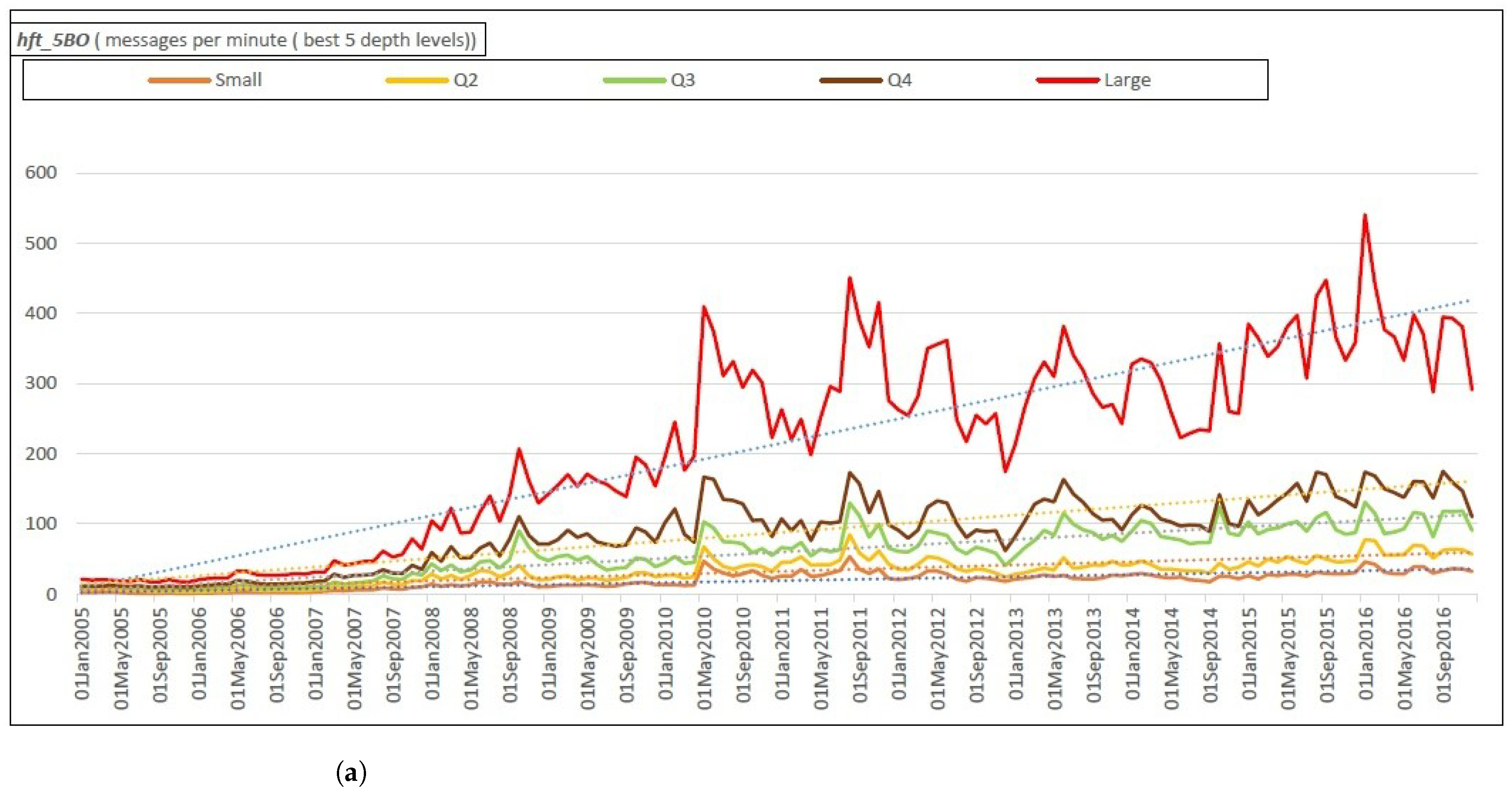
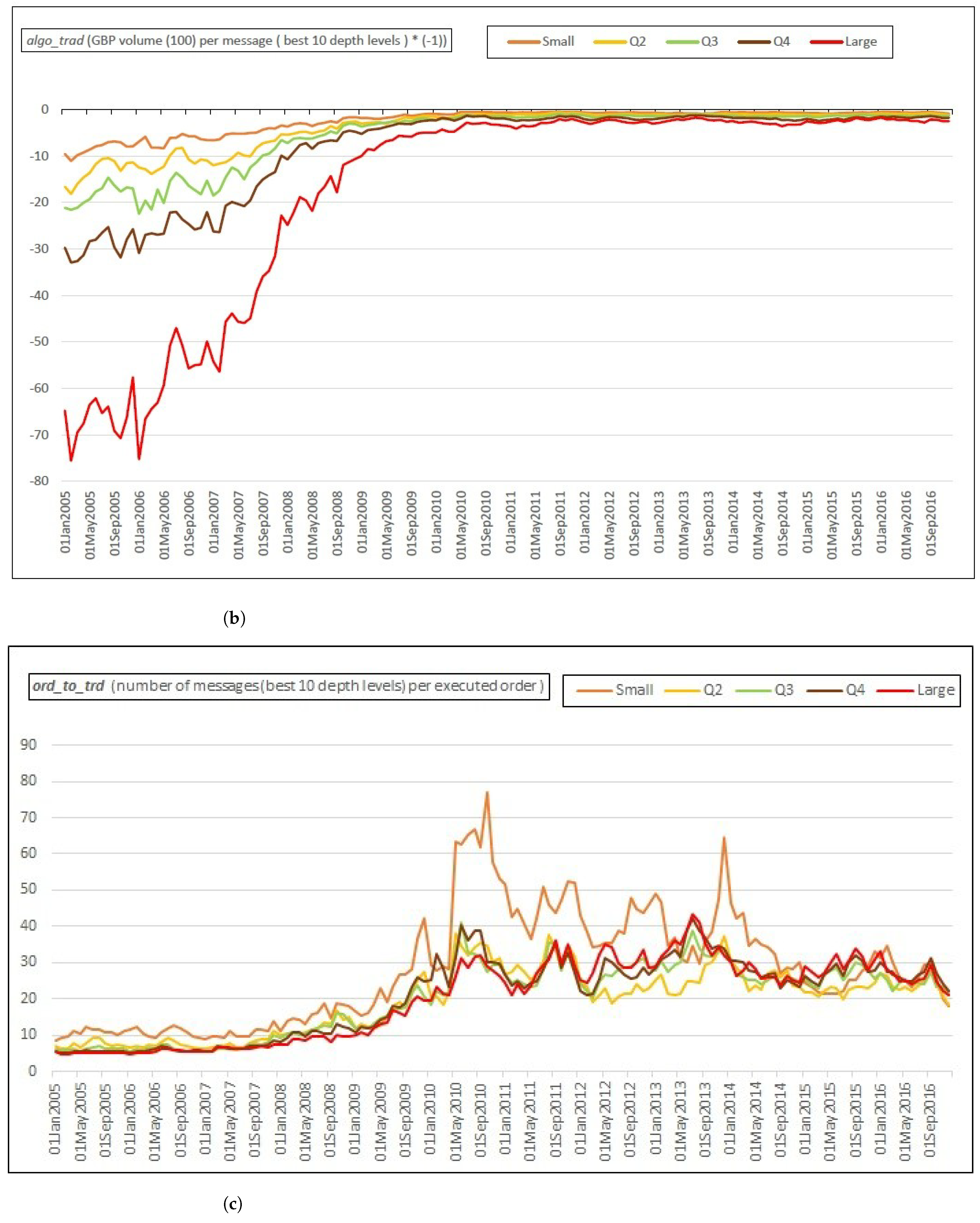
Figure 3.
High-frequency Trading Measures. These figures depict: (
a) the traffic of electronic messages per minute (
b)
Hendershott et al. (
2011)’s proxy of HFT and (
c) order-to-trade ratio.
Figure 3.
High-frequency Trading Measures. These figures depict: (
a) the traffic of electronic messages per minute (
b)
Hendershott et al. (
2011)’s proxy of HFT and (
c) order-to-trade ratio.
Figure 4.
The trading volume fragmentation proxy ().
Figure 4.
The trading volume fragmentation proxy ().
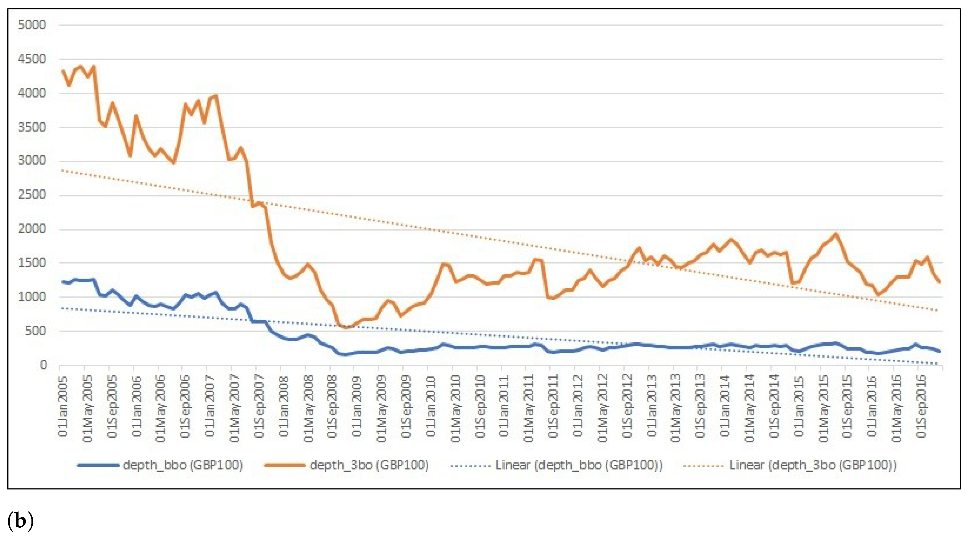
Figure 5.
Liquidity measures. These figures depict three liquidity measures: (a) quoted half-spreads and effective half-spreads; (b) quoted depth at the BBO and 3 best levels. Dotted lines shows the linear trend of these variables.
Figure 5.
Liquidity measures. These figures depict three liquidity measures: (a) quoted half-spreads and effective half-spreads; (b) quoted depth at the BBO and 3 best levels. Dotted lines shows the linear trend of these variables.
Table 1.
The list of all LSE listed sample stocks. The table lists all 149 LSE listed securities (by their RICs) included in the sample for the period 2005–2016 with number of trading days coverage.
Table 1.
The list of all LSE listed sample stocks. The table lists all 149 LSE listed securities (by their RICs) included in the sample for the period 2005–2016 with number of trading days coverage.
| RIC | Days | RIC | Days | RIC | Days | RIC | Days | RIC | Days | RIC | Days |
|---|
| AAL | 3028 | BYG | 2892 | GOG | 2991 | LAND | 3028 | RB | 3029 | SPX | 2973 |
| ABF | 3027 | CCL | 3028 | GPOR | 2989 | LGEN | 3028 | RBS | 3028 | SRP | 3017 |
| ADN | 2898 | CLLN | 2989 | GRG | 2977 | LLOY | 3029 | REL | 3028 | SSE | 3028 |
| AHT | 2898 | CNA | 3028 | GRI | 2972 | LSE | 3022 | | 2900 | STAN | 3028 |
| ANTO | 3024 | CNE | 3029 | GSK | 3028 | MCRO | 2855 | RIO | 3028 | SVS | 2968 |
| 2944 | COB | 3024 | HIK | 2816 | MGGT | 3010 | | 2722 | SVT | 3028 |
| 2572 | CPG | 3028 | HLMA | 2993 | MKS | 3028 | ROR | 2973 | SXS | 2977 |
| AV | 3027 | CPI | 3026 | HMSO | 3022 | | 2399 | RR | 3028 | TATE | 3028 |
| AVV | 2814 | CRDA | 2934 | HSBA | 3027 | | 2382 | RRS | 2968 | | 2408 |
| AZN | 3028 | | 2691 | HSV | 2975 | | 2861 | RSA | 3027 | TLW | 3026 |
| BAB | 2917 | DGE | 3028 | HSX | 2972 | MRW | 3028 | RTO | 3028 | TPK | 3004 |
| BARC | 3028 | | 2503 | ICP | 2980 | MTO | 2987 | | 2966 | TSCO | 3028 |
| BATS | 3028 | DOM | 2764 | IGG | 2942 | NEX | 3021 | SBRY | 3028 | | 2397 |
| BBA | 3020 | DRX | 2786 | IHG | 3028 | NG | 2886 | SDR | 3023 | UBM | 3027 |
| BDEV | 3028 | DTY | 2874 | III | 3028 | NXT | 3028 | SGC | 3016 | ULE | 2980 |
| BLND | 3027 | ECM | 3021 | IMI | 3024 | OML | 3023 | SGE | 3028 | ULVR | 3027 |
| BLT | 3027 | ELM | 2882 | INCH | 3021 | PFC | 2838 | | 2427 | UTG | 2956 |
| BNZL | 3027 | EMG | 3028 | INF | 2869 | PFG | 3023 | SHB | 2971 | UU | 3028 |
| BOY | 2986 | | 2581 | INVP | 2991 | PNN | 3009 | SHP | 3028 | VOD | 3029 |
| BP | 3029 | EZJ | 3025 | ITRK | 3008 | PRU | 3027 | | 2646 | WEIR | 2992 |
| BRBY | 3011 | | 2429 | ITV | 3028 | PSN | 3026 | SMDS | 2997 | WG | 2999 |
| BT | 3028 | FGP | 3025 | JLT | 2994 | PSON | 3028 | SMIN | 3028 | WMH | 3027 |
| BVIC | 2789 | GFS | 3022 | JMAT | 3027 | PZC | 2956 | SMWH | 3007 | WPP | 3021 |
| BVS | 3005 | GKN | 3028 | KGF | 3029 | | 2748 | SN | 3028 | WTB | 3017 |
| BWY | 3019 | GNK | 2992 | KIE | 2915 | RAT | 2958 | SNR | 2858 | Total days | 439,583 |
Table 2.
Descriptive statistics for HFT proxies. The table reports the descriptive statistics for all HFT proxies. The sample comprises 149 stocks divided into 5 equal quintiles based on market capitalization.
Table 1 shows the data coverage in details.
Table 2.
Descriptive statistics for HFT proxies. The table reports the descriptive statistics for all HFT proxies. The sample comprises 149 stocks divided into 5 equal quintiles based on market capitalization.
Table 1 shows the data coverage in details.
| HFT Proxy | Description | Statistics | All | Small | Q2 | Q3 | Q4 | Large |
|---|
| messages per minute (best 10 depth levels) | Mean | 100.36 | 23.77 | 38.97 | 72.39 | 103.80 | 266.31 |
| Median | 47.62 | 17.95 | 30.57 | 56.44 | 90.99 | 171.75 |
| StdDev | 157.77 | 23.22 | 38.25 | 67.59 | 84.81 | 271.25 |
| messages per minute (best 5 depth levels) | Mean | 83.72 | 19.35 | 32.61 | 60.80 | 89.36 | 219.40 |
| Median | 41.10 | 14.42 | 26.09 | 49.34 | 80.49 | 149.97 |
| StdDev | 126.10 | 19.37 | 30.18 | 52.20 | 68.56 | 213.53 |
| messages per minute (BBO) | Mean | 39.32 | 9.57 | 15.67 | 28.33 | 43.50 | 100.91 |
| Median | 20.38 | 7.48 | 12.87 | 23.91 | 40.04 | 76.56 |
| StdDev | 54.32 | 8.98 | 13.09 | 21.76 | 30.81 | 88.30 |
| number of messages for the 10 best levels per executed order (order-to-trade ratio) | Mean | 22.02 | 28.05 | 19.51 | 20.45 | 21.18 | 20.73 |
| Median | 19.06 | 19.97 | 17.28 | 18.46 | 20.40 | 19.83 |
| StdDev | 21.25 | 36.67 | 15.59 | 14.76 | 13.57 | 13.84 |
| GBP volume (100) per message (best 10 depth levels) time (−1) | Mean | −6.93 | −2.24 | −3.73 | −5.14 | −7.51 | −16.21 |
| Median | −1.96 | −0.88 | −1.37 | −1.77 | −2.38 | −3.60 |
| StdDev | 15.51 | 4.19 | 5.87 | 8.42 | 10.93 | 29.12 |
| GBP volume (100) per message (best 5 depth levels) time (−1) | Mean | −7.54 | −2.80 | −4.17 | −5.53 | −8.04 | −17.37 |
| Median | −2.33 | −1.10 | −1.64 | −2.05 | −2.72 | −4.19 |
| StdDev | 16.22 | 5.30 | 6.32 | 8.78 | 11.36 | 30.28 |
| observations (stock * day) | 439,583 | 90,046 | 88,374 | 87,239 | 86,786 | 87,138 |
Table 3.
Pearson’s correlation coefficient matrix. The table reports the Pearson correlation coefficient matrix for the variables calculated on the same balanced sample employed in the regression analyses. The sample comprises 132 stocks for the period December 2005–December 2016 (2624 days). , , and represent the per minute electronic message rate for the 10 best, 5 best, and best bid and offer (BBO) depth levels in the limit order book, respectively, is the Herfindhal–Hirchman index (HHI) showing the degree of market fragmentation, is the time-weighted daily quoted spread in basis point, is the volume weighted effective half-spread in basis point, is the average BBO-level quoted depth measured in GBP100, is the average cumulative depth up to three best limit prices measured in GBP100, is the intraday mid-price range volatility measured in basis point, is the average market capitalization measured in million GBP, is the daily average price level measured in GBX. All are daily measures constructed from the intraday millisecond records.
| Variables | log(hft_10bo) | log(hft_5bo) | log(hft_bbo) | HHItrd | log(spread_bps) | log(espread) | log(depth_bbo) | log(depth_3bo) | Log(mktcap) | log(voltintra) | invprice |
|---|
| log(hft_10bo) | 1 | | | | | | | | | | |
| log(hft_5bo) | 0.996 | | | | | | | | | | |
| log(hft_bbo) | 0.981 | 0.988 | | | | | | | | | |
| HHItrd | 0.561 | 0.546 | 0.503 | | | | | | | | |
| log(spread_bps) | −0.762 | −0.776 | −0.772 | −0.402 | | | | | | | |
| Log(espread) | −0.757 | −0.766 | −0.754 | −0.451 | 0.955 | | | | | | |
| log(depth_bbo) | 0.346 | 0.381 | 0.432 | −0.095 | −0.523 | −0.408 | | | | | |
| log(depth_3bo) | 0.444 | 0.473 | 0.513 | 0.078 | −0.593 | −0.488 | 0.969 | | | | |
| Log(mktcap) | 0.740 | 0.754 | 0.772 | 0.271 | −0.829 | −0.773 | 0.722 | 0.768 | | | |
| log(voltintra) | −0.020 | −0.027 | −0.012 | −0.241 | 0.360 | 0.372 | −0.215 | −0.276 | −0.234 | | |
| invprice | −0.103 | −0.108 | −0.114 | −0.086 | 0.235 | 0.257 | −0.158 | −0.185 | −0.156 | 0.214 | 1.000 |
| all coefficients are significant at 1% level. |
Table 4.
Descriptive Statistics for regression variables. The table presents the descriptive statistics calculated using the balanced sample of 132 stocks for all variables employed in the regression analyses for the period 2005–2016. , , and represent the per minute quote update for the best 10, best 5, and best bid and offer (BBO) depth levels in the limit order, respectively, is the Herfindhal–Hirchman index (HHI) showing the degree of market fragmentation, is the time-weighted daily quoted spread in basis point, is the volume weighted effective half-spread in basis point, is the average BBO level quoted depth measured in GBP100, is the average cumulative depth up to three best limit price measured in GBP100, is the intraday mid price range volatility measured in basis point, is the average market capitalization measured in million GBP, is the daily average price level measured in GBX. All are daily measures constructed from the intraday millisecond records. The table presents the reference value (mean) for all regression estimates.
| Variables | Description | Mean | Median | Std. Dev. | N |
|---|
| spread_bps | quoted half-spreads | 18.37 | 13.14 | 19.83 | 346,368 |
| espread | effective half-spread | 6.41 | 4.87 | 6.92 | 346,368 |
| depth_bbo | average depth (at BBO/GBP100) | 358.15 | 180.23 | 869.90 | 346,368 |
| depth_3bbo | average cumulative depth (best three levels/GBP100) | 1636.19 | 803.05 | 3613.90 | 346,368 |
| hft_10bo | electronic message rate per minute (the best 10 depth levels) | 114.88 | 58.75 | 169.13 | 346,368 |
| hft_5bo | electronic message rate per minute (the best 5 depth levels) | 95.91 | 51.22 | 135.38 | 346,368 |
| hft_bbo | electronic message rate per minute (at BBO) | 44.88 | 25.34 | 58.11 | 346,368 |
| HHItrd | Herfindhal Index (proxy for trade fragmenatation) | 2.17 | 2.38 | 0.74 | 346,368 |
| mktcap | market capitalization (million GBP) | 9666.37 | 3018.93 | 17,853.14 | 346,368 |
| voltintra | Intraday volatility | 286.23 | 216.32 | 542.32 | 346,368 |
| price | daily average price (GBX) | 934.35 | 598.07 | 973.37 | 346,368 |
Table 5.
Effects of HFT (electronic message traffic rate/minute for the 10 best levels) on market liquidity as measured by relative quoted half-spreads and effective half-spreads). The table reports the panel regression estimates for Models 1–3 where the first two liquidity measures ( and ) are regressed on HFT (), market fragmentation () proxy. represents the per minute daily quote update for the best 10 depth levels in the limit order book. is the Herfindhal–Hirchman index (HHI), showing the degree of market fragmentation. The liquidity measures are time-weighted quoted spread (), volume-weighted effective-half spread (). Dependent variables, and are natural log transformed, all spreads-based measures are in basis point. Control variables are natural log transformed market capitalization (), natural log normalized intraday mid-price volatility (), and inverse of the average daily price level (). The regression is based on a balanced panel of 132 stocks and 2624 days (December 2005–December 2016) and has both time (daily) and stock fixed effects. Coefficient estimates are OLS, t-statistics shown in the parentheses below the coefficient, calculated using Newey–West (HAC) for standard errors, a heteroscedasticity and autocorrelation consistent covariance matrix estimator (lags are optimally determined). *** denotes significance at 1% level.
| | I | II | III | IV | V | VI |
|---|
| | | |
| Explanatory Variables | Model-1 | Model-2 | Model-3 | Model-1 | Model-2 | Model-3 |
| −0.278 *** | −0.279 *** | −0.275 *** | −0.32 *** | −0.321 *** | −0.279 *** |
| | (−89.68) | (−90.04) | (−50.21) | (−98.95) | (−99.46) | (−48.42) |
| HHItrd | | 0.049 *** | 0.057 *** | | 0.061 *** | 0.139 *** |
| | | (15.9) | (7.21) | | (18.99) | (16.6) |
| | | −0.002 | | | −0.019 *** |
| | | | (−1.15) | | | (−10.19) |
| log(mktcap) | −0.214 *** | −0.217 *** | −0.218 *** | −0.141 *** | −0.145 *** | −0.153 *** |
| | (−52.76) | (−53.5) | (−53.34) | (−32.87) | (−33.83) | (−35.53) |
| log(voltintra) | 0.165 *** | 0.167 *** | 0.167 *** | 0.211 *** | 0.213 *** | 0.21 *** |
| | (56.69) | (58.17) | (57.84) | (62.68) | (64.4) | (62.98) |
| invprice | 17.751 *** | 17.802 *** | 17.883 *** | 20.303 *** | 20.367 *** | 21.119 *** |
| | (23.43) | (23.41) | (23.38) | (22.68) | (22.69) | (23.35) |
| stock/firm fixed effect | YES | YES | YES | YES | YES | YES |
| time fixed effect | YES | YES | YES | YES | YES | YES |
| Observations | 346,368 | 346,368 | 346,368 | 346,368 | 346,368 | 346,368 |
| R-Square | 0.87 | 0.87 | 0.87 | 0.84 | 0.84 | 0.84 |
Table 6.
Effect of HFT (electronic message rate/minute for the 10 best levels) on market liquidity as measured by the market depth at BBO and the cumulative market depth for 3 best depth levels. The table reports the panel regression results of Models 1–3 where two depth-based liquidity measures ( and ) are regressed on HFT () and market fragmentation () proxy. represents the per minute daily quote update in the 10 best depth levels of the limit order book. is the Herfindhal–Hirchman index (HHI), shows the degree of market fragmentation. The liquidity measures (response variables) are the average quoted depth at best limit price (), and the accumulated average quoted depth up to the best three limit price ( ). All explanatory variables are natural log transformed, and depth measures are in GBP100. Control variables are log market capitalization (), natural log normalized intraday mid-price volatility (), and inverse of the average daily price level (). The regression is based on a balanced panel of 132 stocks and 2624 days (December 2005–December 2016) and has both time (day) and stock (firm) fixed effects. Coefficient estimates are OLS, t-statistics shown in the parentheses below the coefficient, calculated using Newey–West (HAC) for standard errors, a heteroscedasticity and autocorrelation consistent covariance matrix estimator (lags are optimally determined). *** denotes significance at 1% level.
| | I | II | III | IV | V | VI |
|---|
| | | |
| Explanatory Variables | Model-1 | Model-2 | Model-3 | Model-1 | Model-2 | Model-3 |
| ) | −0.284 *** | −0.282 *** | −0.183 *** | −0.295 *** | −0.295 *** | −0.285 *** |
| | (−45.35) | (−45.25) | (−16.13) | (−43.27) | (−43.22) | (−22.7) |
| | −0.107 *** | 0.078 *** | | 0.001 | 0.019 |
| | | (−19.94) | (4.76) | | (0.21) | (1.05) |
| | | −0.045 *** | | | −0.004 |
| | | | (−10.99) | | | (−0.98) |
| 0.816 *** | 0.823 *** | 0.804 *** | 0.864 *** | 0.864 *** | 0.862 *** |
| | (87.13) | (87.53) | (87.28) | (83.64) | (83.4) | (84.29) |
| 0.041 *** | 0.037 *** | 0.029 *** | 0.003 | 0.003 | 0.002 |
| | (10.77) | (9.52) | (7.39) | (0.73) | (0.74) | (0.55) |
| 1.067 | 0.957 | 2.739 | −0.144 | −0.143 | 0.032 |
| | (0.56) | (0.51) | (1.46) | (−0.08) | (−0.08) | (0.02) |
| stock/firm fixed effect | YES | YES | YES | YES | YES | YES |
| time fixed effect | YES | YES | YES | YES | YES | YES |
| observations | 346,368 | 346,368 | 346,368 | 346,368 | 346,368 | 346,368 |
| R-Square | 0.82 | 0.82 | 0.83 | 0.81 | 0.81 | 0.81 |
Table 7.
Effect of HFT (electronic message traffic rate/minute for 5 best levels) on market liquidity as measured by quoted spreads and effective spreads). The table presents the panel regression results of Models 1–3 where first two liquidity measures ( and ) are regressed on HFT () and market fragmentation () proxy. represents the per minute daily quote update for the best 5 depth levels in the limit order book. is the Herfindhal–Hirchman index (HHI), showing the degree of market fragmentation. The liquidity measures are time-weighted quoted spread (), volume-weighted effective-half spread (). Dependent variables, , are natural log transformed, all spreads-based measures are in basis point. Control variables are lnatural og transformed market capitalization (), natural log normalized intraday mid-price volatility () and inverse of the average daily price level (). The regression is based on a balanced panel of 132 stocks and 2624 days (December 2005–December 2016) and has both time (daily) and stock fixed effects. Coefficient estimates are OLS, t-statistics shown in the parentheses below the coefficient, calculated using Newey–West (HAC) for standard errors, a heteroscedasticity and autocorrelation consistent covariance matrix estimator (lags are optimally determined). *** denotes significance at 1% level.
| | I | II | III | IV | V | VI |
|---|
| | | | | | | |
| Explanatory Variables | Model-1 | Model-2 | Model-3 | Model-1 | Model-2 | Model-3 |
| −0.288 *** | −0.289 *** | −0.283 *** | −0.322 *** | −0.324 *** | −0.282 *** |
| | (−92.96) | (−93.21) | (−54.74) | (−99.98) | (−100.38) | (−51.56) |
| | 0.052 *** | 0.065 *** | | 0.065 *** | 0.144 *** |
| | | (17.72) | (9.09) | | (20.72) | (18.81) |
| | | −0.003 * | | | −0.02 *** |
| | | | (−1.96) | | | (−11.24) |
| −0.198 *** | −0.201 *** | −0.202 *** | −0.127 *** | −0.131 *** | −0.139 *** |
| | (−49.14) | (−49.93) | (−49.97) | (−29.43) | (−30.41) | (−32.17) |
| 0.167 *** | 0.169 *** | 0.168 *** | 0.21 *** | 0.213 *** | 0.209 *** |
| | (58.38) | (59.99) | (59.69) | (63.96) | (65.83) | (64.35) |
| 17.159 *** | 17.205 *** | 17.335 *** | 19.847 *** | 19.904 *** | 20.694 *** |
| | (22.65) | (22.68) | (22.7) | (21.99) | (22.04) | (22.83) |
| stock/firm fixed effect | YES | YES | YES | YES | YES | YES |
| time fixed effect | YES | YES | YES | YES | YES | YES |
| Observations | 346,368 | 346,368 | 346,368 | 346,368 | 346,368 | 346,368 |
| R-Square | 0.87 | 0.87 | 0.87 | 0.84 | 0.84 | 0.84 |
Table 8.
Effect of HFT (electronic message traffic rate/minute for 5 best levels) on market liquidity as measured by the marker depth at BBO and the cumulative market depth for 3 best depth levels). The table presents the panel regression results of Models 1–3 where two depth-based liquidity measures ( and ) are regressed on HFT () and market fragmentation () proxy. represents the per minute quote update for the best 5 depth levels in the limit order book. is the Herfindhal–Hirchman index (HHI), showing the degree of market fragmentation. The liquidity measures are the average quoted depth at best limit price (), the accumulated average quoted depth up to the best three limit price ( ). All dependent variables are log transformed and depth measures are in 100GBP. Control variables are log market capitalization (), log normalized intraday mid-price volatility () and inverse of the average daily price level (). The regression is based on a balanced panel of 132 stocks and 2624 days (December 2005–December 2016) and has both time (daily) and stock fixed effects. Coefficient estimates are OLS, t-statistics shown in the parentheses below the coefficient, calculated using Newey–West (HAC) for standard errors, a heteroscedasticity and autocorrelation consistent covariance matrix estimator (lags are optimally determined). *** and * denote significance at 1% and 10% levels, respectively.
| | I | II | III | IV | V | VI |
|---|
| | | | | | | |
| Explanatory Variables | Model-1 | Model-2 | Model-3 | Model-1 | Model-2 | Model-3 |
| −0.25 *** | −0.247 *** | −0.155 *** | −0.268 *** | −0.268 *** | −0.264 *** |
| | (−40.36) | (−40.14) | (−14.76) | (−39.84) | (−39.78) | (−22.66) |
| | −0.105 *** | 0.068 *** | | 0.003 | 0.01 |
| | | (−19.51) | (4.5) | | (0.52) | (0.62) |
| | | −0.044 *** | | | −0.002 |
| | | | (−11.27) | | | (−0.43) |
| 0.811 *** | 0.818 *** | 0.801 *** | 0.863 *** | 0.863 *** | 0.862 *** |
| | (85.82) | (86.18) | (86.22) | (82.97) | (82.75) | (83.75) |
| 0.029 *** | 0.025 *** | 0.018 *** | −0.007 * | −0.007 * | −0.007 * |
| | (7.69) | (6.42) | (4.59) | (−1.71) | (−1.68) | (−1.75) |
| 1.584 | 1.492 | 3.227 * | 0.173 | 0.176 | 0.249 |
| | (0.82) | (0.77) | (1.69) | (0.09) | (0.09) | (0.13) |
| stock/firm fixed effect | YES | YES | YES | YES | YES | YES |
| time fixed effect | YES | YES | YES | YES | YES | YES |
| Observations | 346,368 | 346,368 | 346,368 | 346,368 | 346,368 | 346,368 |
| R-Square | 0.82 | 0.82 | 0.82 | 0.81 | 0.81 | 0.81 |
Table 9.
Effect of HFT (electronic message traffic rate/minute at BBO ) on market liquidity as measured by relative quoted spreads and effective half-spreads. The table presents the panel regression results of Models 1–3 where the first two liquidity measures ( and ) are regressed on HFT (), market fragmentation () proxy. represents the per minute quote update for the BBO depth levels in the limit order book. is the Herfindhal–Hirchman index (HHI), shows the degree of market fragmentation. The liquidity measures are time-weighted quoted spread (), volume-weighted effective-half spread (). Dependent variables, , are log transformed, all spreads-based measures are in basis point. Control variables are natural log transformed market capitalization (), natural log normalized intraday mid-price volatility (), and inverse of the average daily price level (). The regression is based on a balanced panel of 132 stocks and 2624 days (December 2005–December 2016) and has both time (daily) and stock fixed effects. Coefficient estimates are OLS, t-statistics shown in the parentheses below the coefficient, calculated using Newey–West (HAC) for standard errors, a heteroscedasticity and autocorrelation consistent covariance matrix estimator (lags are optimally determined). *** denotes significance at 1% level.
| | I | II | III | IV | V | VI |
|---|
| | | | |
| Explanatory Variables | Model-1 | Model-2 | Model-3 | Model-1 | Model-2 | Model-3 |
| −0.269 *** | −0.269 *** | −0.265 *** | −0.291 *** | −0.292 *** | −0.254 *** |
| | (−81.77) | (−81.87) | (−48.72) | (−84.2) | (−84.41) | (−42.99) |
| | 0.047 *** | 0.054 *** | | 0.059 *** | 0.118 *** |
| | | (15.35) | (8.35) | | (17.78) | (17.05) |
| | | −0.002 | | | −0.018 *** |
| | | | (−1.08) | | | (−9.68) |
| −0.203 *** | −0.207 *** | −0.207 *** | −0.138 *** | −0.142 *** | −0.148 *** |
| | (−47.98) | (−48.64) | (−48.46) | (−29.98) | (−30.81) | (−32.15) |
| 0.162 *** | 0.164 *** | 0.164 *** | 0.202 *** | 0.204 *** | 0.202 *** |
| | (55.6) | (57) | (56.79) | (60.4) | (62.03) | (60.66 |
| 17.29 *** | 17.338 *** | 17.406 *** | 20.246 *** | 20.306 *** | 20.963 *** |
| | (20.89) | (20.87) | (20.85) | (20.3) | (20.3) | (20.93) |
| stock/firm fixed effect | YES | YES | YES | YES | YES | YES |
| time fixed effect | YES | YES | YES | YES | YES | YES |
| Observations | 346,368 | 346,368 | 346,368 | 346,368 | 346,368 | 346,368 |
| R-Square | 0.87 | 0.87 | 0.87 | 0.83 | 0.83 | 0.83 |
Table 10.
Effect of HFT (electronic message traffic rate/minute at BBO) on market liquidity as measured by the marker depth at BBO and the cumulative market depth for 3 best depth levels). The table presents the panel regression results of Models 1–3 where two depth-based liquidity measures ( and ) are regressed on HFT () and market fragmentation () proxy. represents the per minute daily quote update for the BBO in the limit order book. is the Herfindhal–Hirchman index (HHI), which shows the degree of market fragmentation. The liquidity measures are the average quoted depth at best limit price (), the accumulated average quoted depth up to the best three limit price ( ). All dependent variables are natural log transformed and depth measures are in 100GBP. Control variables are natural log market capitalization (), natural log normalized intraday mid-price volatility (), and inverse of the average daily price level (). The regression is based on a balanced panel of 132 stocks and 2624 days (December 2005–December 2016) and has both time (daily) and stock fixed effects. Coefficient estimates are OLS, t-statistics shown in the parentheses below the coefficient, calculated using Newey–West (HAC) for standard errors, a heteroscedasticity and autocorrelation consistent covariance matrix estimator (lags are optimally determined). ***, **, * denote significance at 1%, 5%, and 10% levels, respectively.
| | I | II | III | IV | V | VI |
|---|
| | Log(depth_bbo) | Log(depth_3bo) |
| Explanatory Variables | Model-1 | Model-2 | Model-3 | Model-1 | Model-2 | Model-3 |
| −0.148 *** | −0.146 *** | −0.07 *** | −0.184 *** | −0.184 *** | −0.188 *** |
| | (−24.55) | (−24.45) | (−6.76) | (−27.66) | (−27.63) | (−16.19) |
| | −0.112 *** | 0.007 | | −0.004 | −0.01 |
| | | (−20.37) | (0.52) | | (−0.57) | (−0.74) |
| | | −0.037 *** | | | 0.002 |
| | | | (−9.4) | | | −0.5 |
| 0.764 *** | 0.771 *** | 0.758 *** | 0.825 *** | 0.825 *** | 0.826 *** |
| | (79.74) | (80.22) | (80.13) | −78.28 | −78.11 | −78.92 |
| −0.002 | −0.007 * | −0.012 *** | −0.032 *** | −0.032 *** | −0.032 *** |
| | (−0.46) | (−1.72) | (−3.05) | (−7.89) | (−7.93) | (−7.85) |
| 3.97 * | 3.856 * | 5.173 ** | 2.066 | 2.063 | 1.986 |
| | (1.92) | (1.88) | (2.53) | −1.02 | −1.02 | −0.97 |
| stock/firm fixed effect | YES | YES | YES | YES | YES | YES |
| time fixed effect | YES | YES | YES | YES | YES | YES |
| Observations | 346,368 | 346,368 | 346,368 | 346,368 | 346,368 | 346,368 |
| R-Square | 0.82 | 0.82 | 0.82 | 0.81 | 0.81 | 0.81 |
Table 11.
Effects of HFT on liquidity: summary estimates. The table summarize the estimates reported in
Table 5,
Table 6,
Table 7,
Table 8,
Table 9 and
Table 10 for Model 3. *** and * denote significance at 1%, and 10% levels, respectively.
Table 11.
Effects of HFT on liquidity: summary estimates. The table summarize the estimates reported in
Table 5,
Table 6,
Table 7,
Table 8,
Table 9 and
Table 10 for Model 3. *** and * denote significance at 1%, and 10% levels, respectively.
| | | | | |
|---|
| LOB Depth Level | | | | | | | | | | | | |
| −0.265 *** | −0.283 *** | −0.275 *** | −0.254 *** | −0.282 *** | −0.279 *** | −0.07 *** | −0.155 *** | −0.183 *** | −0.188 *** | − 0.264*** | −0.285 *** |
| | (−48.72) | (−54.74) | (−50.21) | (−42.99) | (−51.56) | (−48.42) | (−6.76) | (−14.76) | (−16.13) | (−16.19) | (−22.66) | (−22.7) |
| 0.054 *** | 0.065 *** | 0.057 *** | 0.118 *** | 0.144 *** | 0.139 *** | 0.007 | 0.068 *** | 0.078 *** | −0.01 | 0.01 | 0.019 |
| | (8.35) | (9.09) | (7.21) | (17.05) | (18.81) | (16.6) | (0.52) | (4.5) | (4.76) | (−0.74) | (0.62) | (1.05) |
| * HHItrd | −0.002 | −0.003 * | −0.002 | −0.018 *** | −0.02 *** | −0.019 *** | −0.037 *** | −0.044 *** | −0.045 *** | 0.002 | −0.002 | −0.004 |
| | (−1.08) | (−1.96) | (−1.15) | (−9.68) | (−11.24) | (−10.19) | (−9.4) | (−11.27) | (−10.99) | −0.5 | (−0.43) | (−0.98) |
| −0.207 *** | −0.202 *** | −0.218 *** | −0.148 *** | −0.139 *** | −0.153 *** | 0.758 *** | 0.801 *** | 0.804 *** | 0.826 *** | 0.862 *** | 0.862 *** |
| | (−48.46) | (−49.97) | (−53.34) | (−32.15) | (−32.17) | (−35.53) | (80.13) | (86.22) | (87.28) | −78.92 | (83.75) | (84.29) |
| 0.164 *** | 0.168 *** | 0.167 *** | 0.202 *** | 0.209 *** | 0.21 *** | −0.012 *** | 0.018 *** | 0.029 *** | −0.032 *** | −0.007 * | 0.002 |
| | (56.79) | (59.69) | (57.84) | (60.66) | (64.35) | (62.98) | (−3.05) | (4.59) | (7.39) | (−7.85) | (−1.75) | (0.55) |
| 17.406 *** | 17.335 *** | 17.883 *** | 20.963 *** | 20.694 *** | 21.119 *** | 5.173 ** | 3.227 * | 2.739 | 1.986 | 0.249 | 0.032 |
| | (20.85) | (22.7) | (23.38) | (20.93) | (22.83) | (23.35) | (2.53) | (1.69) | (1.46) | −0.97 | (0.13) | (0.02) |
| stock/firm fixed effect | YES | YES | YES | YES | YES | YES | YES | YES | YES | YES | YES | YES |
| time fixed effect | YES | YES | YES | YES | YES | YES | YES | YES | YES | YES | YES | YES |
| observations | 346,368 | 346,368 | 346,368 | 346,368 | 346,368 | 346,368 | 346,368 | 346,368 | 346,368 | 346,368 | 346,368 | 346,368 |
| R-Square | 0.87 | 0.87 | 0.87 | 0.83 | 0.84 | 0.84 | 0.82 | 0.82 | 0.83 | 0.81 | 0.81 | 0.81 |


