Price and Volatility Transmissions among Natural Gas, Fertilizer, and Corn Markets: A Revisit

Abstract

In this paper, we revisit price and volatility transmission among natural gas, fertilizer, and corn markets; an important issue was explored in previous work. An update of the results is urgently needed due to the recent enormous price volatility in the commodities, fertilizer, and energy markets. We followed the same methodology as previous work and used the vector error correction model and the multivariate generalized autoregressive heteroskedasticity model, but we adopted a new methodology to gather higher frequency data for fertilizer to estimate the interactions and examine the mechanisms between these market prices. Our results are consistent with previous research showing that natural gas price returns in the short-term are significantly affected by its lagged returns from itself and corn markets, and it will be affected by its lagged return sand fertilizer markets. However, we did not find a significant relationship among fertilizer, corn, and natural gas markets from May to November 2021. Moreover, the lagged conditional volatility of corn prices will affect the conditional volatility in the natural gas market but not vice versa.

1. Introduction

Commodity markets have experienced intensive price volatility in recent years, especially in 2021. For example, the price of fertilizer rose “moderately by 3%” in 2020 while increased sharply in 2021, which reached near-record high prices, achieving a high level not seen since the 2008–2009 global financial crisis (WorldBank 2020). Other commodities have experienced similar price volatility as fertilizer, e.g., global food prices fell steeply in June and July 2021, and will surge to their highest levels in a decade, by November, or within three months (Alcorn 2021). Natural gas prices in the US have also experienced dramatic fluctuations, reaching their highest prices since the 2005–2006 winter, with a 7-year high of record global prices (EIA 2021). These severe price changes have not only increased the costs of risk management, they also have a negative impact on the economic recovery and growth rates of some countries, especially underdeveloped countries (Jacks et al. 2011).

The goal of this paper was to investigate the price and volatility transmission mechanisms among natural gas, fertilizer, and US corn markets in the ten years (from 2011 to 2021). A novel study by Etienne et al. (2016) identifies the price volatility transmission mechanism among natural gas, ammonia, and corn prices from 1994 to 2014. They find significant correlations between fertilizer and corn prices and a weak relationship between those markets and the natural gas market. They also found that an unidirectional impact of lagged conditional volatility of fertilizer prices (specifically ammonia prices) positively affects the conditional volatility of corn markets. However, given the recent intensive price volatility in the last few years, it is not certain whether such price transmission mechanisms among the three markets remain the same or have changed. Moreover, understanding these mechanisms can assist governments in making targeted policies and possibly help companies manage potential related risks.

To achieve the objective, a vector error correction model (VECM) and multivariate generalized autoregressive conditional heteroskedasticity (MGARCH) framework based on Etienne et al. (2016) was used, but with substantial changes. First, daily frequency data were adopted instead of weekly frequency data, enabling the capture of volatility spillover effects between different markets. Different levels of frequency data may yield inconsistent results, thus working with higher frequency data (i.e., daily) is recommended (Saghaian et al. 2018). Moreover, the sample size was expanded from around 1000 observations (in Etienne et al. (2016)’s research) to more than 2000.

Second, exchange-traded funds (ETF) were used as proxy for fertilizer prices. The World Bank Commodity outlook neither provides US Midwest weekly ammonia prices nor daily frequencies of fertilizer prices; thus, there is a need to look for variables that can become approximate proxies for fertilizer prices. The ETF index was selected because it can reflect the daily performance and general price trends of the major fertilizer suppliers, and it is sensitive to price changes of related raw material commodities (e.g., natural gas prices). This index reflects changes in fertilizer prices since a company’s return is largely dependent on product prices, assuming a constant capacity in the short-term. Moreover, monthly trends regarding monthly fertilizer prices from the International Monetary Fund (IMF) world primary commodity database were inspected and it was found that the fertilizer ETF index and fertilizer prices share a similar trend (IMF 2021), as Figure 1 and Figure 2 show. Thus, fertilizer ETF is a plausible, good proxy for fertilizer prices.

Lastly, the sample period was updated to include the latest date (30 November 2021) reflecting the current price transmission mechanism and providing a timely and practical implication.

Results obtained showed several similarities and differences compared to Etienne et al. (2016). First, results showed that natural gas prices were statistically and significantly affected by their own lagged and corn lagged terms; fertilizer markets were also statistically and significantly affected by natural gas markets. These results are consistent with results from Etienne et al. (2016). However, the relationship between fertilizer prices and corn prices was not found but different results in the corn prices and the fertilizer markets were negatively affected by the natural gas prices (Etienne et al. (2016)’s results show the positive relationships). Third, in the long-term, fertilizer was found to be the only statistically significant parameter between adjustment parameters. This is contrary to Etienne et al. (2016)’s results of strong statistical significant relationships for adjustment parameters and the fertilizer (ammonia) or corn. Moreover, lagged conditional volatility of corn prices was found to affect the conditional volatility of the natural gas market but not vice versa.

The contribution of this paper lies in two parts: first, our work contributes to the existing knowledge on price and volatility transmissions among natural gas, fertilizers, and corn markets by proving their relationships in a recent time period. Second, we adopted a new methodology to gather higher frequency data for fertilizers to examine the mechanisms between these market prices in detail.

The rest of the paper is organized as follows. The following section presents recent literature on price relationships in different markets. Section 3 and Section 4 cover the methodology and data, respectively. Section 5 presents the results, and Section 6 concludes the paper.

2. Literature Review

Recent studies in the past five years on the price relationships between commodity markets of food, energy (such as oil or natural gas), and fertilizer, can be divided into three categories: (i) energy prices and food prices (ii) fertilizer prices and food prices; (iii) energy prices and fertilizer prices. Previous literature has identified the price volatility linkage between energy prices, fertilizer prices, and food prices (e.g., Etienne et al. (2016)). However, more recent literature remains sparse, in regard to how the prices in these three markets are linked.

First, some recent studies have revealed the intercommodity price volatility transmission between energy prices and food prices, but its mechanism remains unclear. On the one hand, some of the literature show their unidirectional relationship and prove such a relationship in the short-term and long-term, respectively. Shahnoushi et al. (2017) showed that crude oil and gasoline prices have a significant positive impact on food price subgroups, such as cereals and meats. With the rise in diammonium phosphate (DAP) and triple superphosphate prices, cereal, beverage, and vegetable oil prices increased. Taghizadeh-Hesary et al. (2018) argued that energy prices (oil price) have a significant impact on food prices and that the shares of oil prices, in agricultural food price volatility, are the largest, according to their results on impulse response functions. Similarly, Ji et al. (2018) showed significant risk spillovers from energy (oil and natural gas) to agricultural commodities (maize, rice, soybean, and wheat) by measuring the conditional value-at-risk (CoVaR) and delta CoVaR. The latter research also conducted by Taghizadeh-Hesary et al. (2019) indicates that food prices will respond positively to any shock from oil prices. Particularly, oil price movements can explain 64.17% of food price variance. The research from Nwoko et al. (2016) revealed a unidirectional causality with causality running from oil price to food price volatility, but not vice versa. Supporting their conclusion, Siami-Namini et al. (2019) studied volatility transmission among oil price, exchange rate, and agricultural commodities prices and concluded that volatility in the agricultural commodity returns for most cases is affected by the volatility of the crude oil returns in the post-crisis period. A recent study by Dutta et al. (2021) investigated the correlation between energy price uncertainty and the Malaysian palm oil industry during the 2014 oil price decline and the COVID-19 outbreak. They concluded that oil market volatility negatively impacts palm oil prices and such an impact intensified during 2014 and the COVID-19 outbreak.

For short-term or long-term relationships, Ibrahim (2015) studied a case from Malaysia and found that positive oil prices exert significant influences on the inflation of food prices in the short-term, and that there is a significant relation between oil price increases and food price in the long-term. Recent work by Radmehr and Rastegari Henneberry (2020) found that both in the short-term and long-term, food prices increase in response to an increase of energy prices. Chowdhury et al. (2021) found that the relationship between energy prices and food prices is nonlinear and asymmetric: in the short-term, food prices are only affected by positive changes in energy prices, while in the long-term, both positive and negative changes in energy prices impact food prices. However, Fowowe (2016) argued that structural break cointegration shows no long-term link between energy and food prices. Meanwhile, nonlinear causality tests show no short-term link between energy and food prices. Meyer et al. (2018) focused on the effects of oil price changes on food prices in oil-exporting developing countries between 2001 and 2014, and found no long-term relation between oil price reduction and food prices. Similarly, Eissa and Al Refai (2019) adopted a nonlinear model to explore the dynamic relationship between oil prices and agricultural commodities (barley, corn, and rapeseed oil) from 1990 to 2018, but did not find correlations in the long-term. Roman et al. (2020) also only found that a short term linkage of crude oil prices occurred with food, cereal, and oil prices between January 1990 and September 2020.

Conversely, Rezitis (2015) used panel VAR methods and Granger causality tests, with results indicating bidirectional panel causality effects between crude oil prices and international agricultural prices, as well as between US exchange rates and international agricultural prices. Su et al. (2019) investigated causalities between oil and agricultural prices in the global market, and found a bidirectional positive causality between oil and agricultural products prices. The evidence from De Gorter and Just (2008) shows that different agricultural shocks can have different effects on oil prices and that corn used in ethanol plays an important role in the impact of corn demand shocks on oil price.

Compared to the studies that explored the relationship between energy prices and food prices, recent research on the correlations between food prices and fertilizer prices are relatively few, despite fertilizer playing an essential role in agricultural production. Some research highlights the important role of fertilizer prices in agricultural commodities prices, but they arrive at mixed results. Dillon and Barrett (2016) found a negligible effect of fertilizer prices in local maize price determination once controlling for changes in global maize prices. However, Ismail et al. (2017) investigated the relationship between the price volatility of food and fertilizer and found that fertilizer prices (urea) positively and significantly affect the mean prices of some agricultural commodities, such as rice and sugar. However, the volatility of fertilizer prices is only transmitted on specific products, such as sunflower oil. Kalkuhl et al. (2016) used an empirical model and concluded that high fertilizer prices and price risk will substantially decrease the global supply response to higher crop prices.

Finally, some studies explored the relationship between energy prices and fertilizer prices. Chen et al. (2012) evaluated the effect of crude oil prices on global fertilizer prices in both mean and volatility, and showed that most fertilizer prices are significantly affected by the crude oil price while the volatility of global fertilizer prices and crude oil price from March to December 2008 were higher than in other periods. Results from Sanyal et al. (2015) showed that changes in oil and natural gas prices increased fertilizer prices from June 2007 to June 2008, suggesting that volatility effects of oil and natural gas prices on fertilizer prices were significant. Wongpiyabovorn (2021) found that natural gas prices strongly influence both ammonia and urea prices during the pre-2010 period.

3. Methodology

Following the methodology in (Etienne et al. 2016)’s paper, a time-series approach was used to examine the linkages among natural gas, fertilizer, and agricultural commodity prices. Several statistical properties were considered before modeling. First, time-series data with non-stationarity properties may result in spurious regression results when using normal approaches (OLS, for instance). Therefore, a first-order difference was applied to address the problem. Second, cointegration may appear among non-stationary variables. Cointegration refers to non-stationary variables having a long-term relationship. Therefore, these variables are to be modeled considering both short-and long-term dynamics. Finally, time-varying and clustering volatility of time series data will violate the standard regression model assumption of being independently and identically distributed ($iid$). This problem is addressed with ARCH and GARCH models.

3.1. The VECM-MGARCH Model

In a similar path, a vector error correction multivariate GARCH model (VECM-MGARCH) is considered in Equation (1), in the case of cointegration, in order to examine the price and volatility spillovers among natural gas, fertilizer, and agricultural commodity prices:

$$\Delta P_t=\sum _{j=1}^p{\beta }_j\Delta P_{t-j}+\alpha EC{T}_{t-1}+{\epsilon }_t$$

(1)

$${\epsilon }_t|I_{t-1}(0,H_t)$$

where $\Delta P_t$ is a $3\times 1$ vector, which includes the first difference of prices of natural gas, fertilizer, and corn prices, ${\beta }_j$ is a $3\times 3$ matrix of autoregressive coefficients that models the short-term dynamics between the three markets, p is the lag length; $ECT$ is the error correction term that measure the three markets’ long-term relationships; $\alpha$ is a $3\times 1$ vector, indicating the the speed of adjustment response in long-term. ${\epsilon }_t$ is a $3\times 1$ vector of error term. $H_t$ is a variance–covariance matrix of error term, the conditioning on past information $I_{t-1}$.

3.2. The BEKK Model

Next, the Baba–Engle–Kraft–Kroner (BEKK) model was used to specify the $H_t$. The advantages of adopting the BEKK model (see Baba et al. 1990; Engle and Kroner 1995 for example) are two-fold: (i) it directly estimates the conditional covariance matrix; (ii) it ensures the positive definiteness of the conditional covariance matrix and reduces the dimension of the parameter vector in $H_t$. Equation (2) is the BEKK model with one lag:

$$H_t=C{C}^{\prime }+A^{\prime }{\epsilon }_{t-1}{\epsilon }_{t-1}^{\prime }A+B^{\prime }{H}_{t-1}B,$$

(2)

where C is a 3 by 3 lower triangular matrix that corresponds to the constant, ${\epsilon }_{t-1}{\epsilon }_{t-1}^{\prime }$ are the squared lagged errors, A is a 3 by 3 matrix of the ARCH parameters containing elements measuring the degree of innovation from one market to another, and B is a 3 by 3 matrix of the GARCH parameters that show persistence in conditional volatility between two markets. After setting up the model, we can estimate them by maximum likelihood procedures (see Seo 2007; Serra et al. 2011).

4. Data

The dataset used comes from different sources, with some being the same sources as Etienne et al. (2016). The fertilizer price was represented by the Solactive Global Fertilizers/Potash Total Return Index, which tracks the performance of the largest and most liquid listed companies globally that are active in some aspect in the fertilizer industry. Such an ETF index may reflect timely price changes in the fertilizer industry, and be a good proxy for fertilizer prices. Besides, non-energy commodities in the commodity index have experienced lower volatility. These data were collected from Yahoo Finance.com. The ammonia price in the US Midwest is not used as a fertilizer price because the dataset from the World Bank commodity market does not provide it at the daily level. For agricultural market commodities, corn was considered, since it is a dominant and common global crop and one of most reliant crops in fertilizer. Yahoo Finance provided the history data. The natural gas prices were the rolling prices of futures contracts traded on the New York Mercantile of Exchange (NYMEX), obtained from the energy information administration (EIA). The three datasets were merged at daily frequencies by matching the date and removing some null values. The sample period was from 25 May to 30 November 2021, since the inception date of fertilizer ETF was 25 May 2011. There were 2219 observations used in this study.

From Figure 3, which plots the three different prices series, we see several important patterns: First, natural gas prices show a general increasing or decreasing trend during some periods before January 2020. This indicates an increasing trend (May 2011–May 2012), constantly rising with some fluctuations (May 2012–March 2014), sharply dropping (March 2014–January 2016), increasing again (January 2016–November 2018), followed by descending (November 2018–January 2020), respectively. Second, corn prices remained relatively stable in some periods (November 2014–December 2019), except for a boom from May to July 2012 and a drop from May 2013 to September 2014. Thirdly, similar to natural gas price fluctuation patterns, fertilizer prices showed increasing or decreasing patterns at certain times, such as falling from January 2011 to January 2014; and sharply increasing from July to November 2018.

We also observed a similar volatility pattern between fertilizer prices and natural gas prices after 2014, which is different from findings in Etienne et al. (2016). Finally, a significantly common upward-trending pattern was observed in natural gas and corn prices in January 2020. Previous research has explained that such price trends for natural gas may be the consequence of preceding warm winters; thus, market players have been less optimistic and more cautious about future investments as they had already expected lower sales (Nyga-Łukaszewska and Aruga 2020).

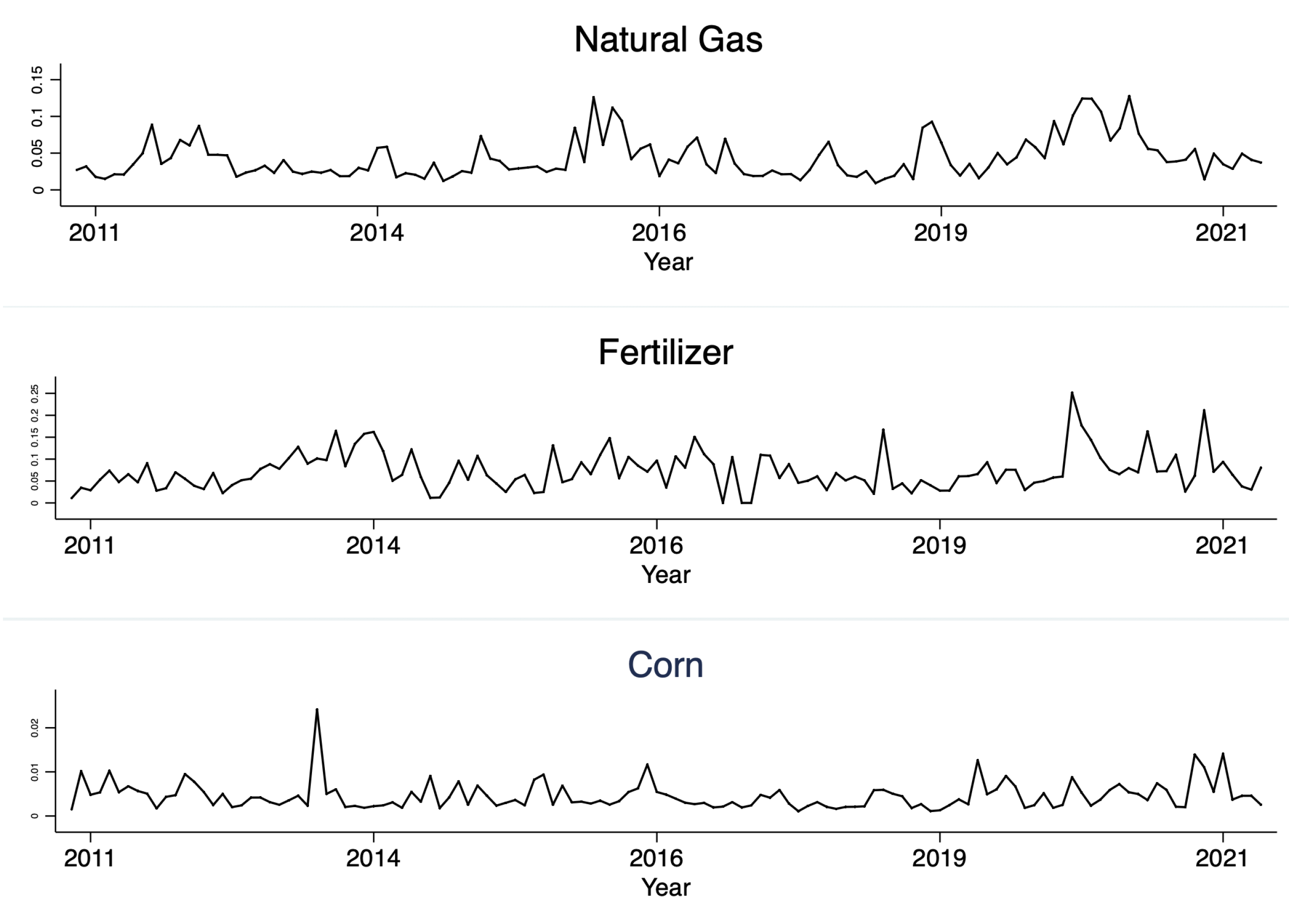
Figure 4 plots the one-month rolling coefficient of variation (standard deviation divided by mean) for natural gas, fertilizer, and corn prices, respectively. The coefficient of variation is used to compare the volatility of these price series. After adopting data at the daily level, several results were found to be different from Etienne et al. (2016). First, the range of coefficient of the variation was significantly smaller than from Etienne et al. (2016). This may mean that estimates of the relationship between different markets may reflect more accurately the volatility of prices because of daily level data. Second, in contrast to the positive correlation of volatility of the three prices in previous research, Figure 2 suggests that they only show correlations in a specific period, such as from November 2011 to January 2012 and January 2020 to January 2021.

For natural gas prices from December 2015 to January 2016, significant price volatility was experienced compared to other commodities. The coefficient of variation continued to decline during the pandemic of COVID-19. For the fertilizer price, its coefficient of variation showed peaks in December 2019 followed by three months of decline until March 2020. For corn prices, the coefficient of variation was stable (around 0.005), and its range of variation was the smallest among the three markets. Meanwhile, unlike the corn’s coefficient of variation in previous research, in this study it only peaked in July 2013 and quickly returned to a smaller value (0.005) within a month. Although the coefficient of corn prices fluctuated due to the pandemic, the degree of variation was less than 0.015.

For stationarity testing, the augmented Dickey–Fuller (ADF) and Phillips–Perron (PP) tests were applied to the three price series. The lag length of the ADF test was selected according to the Akaike information criterion (AIC). All prices were adjusted to logarithmic scales. Results show a failure to reject the null hypothesis of non-stationarity at the 5% significance level for any three log price series. All prices returned at first differences are stationary at the 5% significant level.

Table 1. Descriptive statistics of natural gas, fertilizer, and corn returns (2011–2021).

	Natural Gas Return	Fertilizers Return	Corn Return
Panel (a) summary statistics
Observations	2218	2218	2218
Mean	0.00	−0.03	−0.01
Std. Dev.	3.27	6.67	1.86
Minimum	−18.05	−35.66	−25.2
Maximum	19.8	40.55	8.9
Skewness	0.03 ***	0.28 ***	−0.98 ***
Excess kurtosis	6.40 ***	5.99 ***	17.1 ***
Jarque–Bera	1071.21 ***	856.50 ***	19,000 ***
Panel (b) return correlation coefficients
AC(1)	−0.0558 ***	−0.249 ***	0.0277
AC(2)	0.00305	−0.286 ***	−0.0387 **
Ljung–Box(6)	11.03 **	155.62 ***	13.38 ***
Ljung–Box(12)	21.85 ***	169.10 ***	19.76 **
Panel (c) squared return correlation
AC(1)	0.141 ***	0.146 ***	0.00963
AC(2)	0.0710 ***	0.00525	0.0311 **
Ljung–Box(6)	185.28 ***	66.74 ***	12.5 **
Ljung–Box(12)	272.93 ***	106.79 ***	17.87
Panel (d) unit root test results
ADF	−49.73 ***	−60.69 ***	−45.76 ***
PP	−49.79 **	−65.06 ***	−45.75 ***

Note: returns are calculated as $log(p_t/p_{t-1})\times 100$. ADF and PP stand for augmented Dickey–Fuller and Phillips Perron tests, respectively. AC is the autocorrelation coefficient. Ljung–Box is the test for autocorrelation of the returns and squared return series, computed with 6 and 12 lags, respectively. The t-statistics are denoted as *** $p<$ 0.01, ** $p<$ 0.05, respectively.

shows the descriptive statistics of price returns, multiplied by 100, for each of the three commodities. In panel (a), the average returns of three commodities are observed to be similar to each other, all being close to zero. Although natural gas has the highest average price return, the average return difference between the natural gas and the other two commodities was less than 0.1. In contrast to Etienne et al. (2016), the price return of the fertilizer market was the most volatile commodity compared to other commodities, which is consistent with the patterns observed in Figure 2. Results from the Jarque–Bera test and excess kurtosis indicate that all return series may not be normally distributed. The statistically significant results in panel (b) and panel (c) are the same as Etienne et al. (2016), which show the rejection of the null hypothesis, and no autocorrelation for both returns and squared returns.

To determine if a potential cointegrating relationship existed, the Johansen maximum likelihood test was applied, with results in

Table 2. Johansen maximum likelihood test of cointegrating relationship among natural gas, fertilizer, and corn prices (2011–2021).

Maximum Rank (K)	Log-Likelihood	Eigenvalue	Trace Statistic	5% Critical Value	1% Critical Value
0	13,058.74		35.41	29.68	35.65
1	13,069.28	0.01	14.33	15.41	20.04
2	13,073.91	0.004	5.09	3.76	6.65
3	13,076.45	0.002

Note: the null hypothesis for each row is that the three prices have a maximum of a K cointegrating vector (measured in logarithmic format). When the trace statistic reaches the crucial value, the null hypothesis is rejected.

. Based on AIC, a maximum lag of 26 (26 days) was selected. Results suggest rejecting the null hypothesis of no cointegrating vector between three markets at the 5% significance level. However, one cointegrating vector exists for three commodity prices as the trace statistic is between the 5% critical value and 1% critical value. As a result, a vector error correction model (VECM) should be employed to account for the long-term relationship.

5. Estimation Results

Table 3. VECM-MGARCH Model Estimation Results (2011–2021).

Panel (a) Error Correction Term
$EC{T}_t=0.004P{\left(NG\right)}_t-0.048$ *** $p{\left(Fertilizer\right)}_t+0.026$ *** $p{\left(Corn\right)}_t+0.104$
Panel (b) Vector Error Correction Model
	Natural Gas ($i=1$)	Fertilizer ($i=2$)	Corn ($i=3$)
$\Delta p{\left(NG\right)}_{t-1}$	−0.709 ***	−0.0599 *	0.00275
	(0.0201)	(0.0339)	(0.0115)
$\Delta p{\left(NG\right)}_{t-2}$	−0.338 ***	−0.0310	−0.0141
	(0.0200)	(0.0338)	(0.0115)
$\Delta p{\left(Fertilizer\right)}_{t-1}$	−0.0178	0.239 ***	0.00171
	(0.0205)	(0.0345)	(0.0117)
$\Delta p{\left(Fertilizer\right)}_{t-2}$	−0.0202	0.0712 ***	0.00882
	(0.0126)	(0.0213)	(0.00722)
$\Delta p{\left(Corn\right)}_{t-1}$	0.0848 **	-0.0113	−0.619 ***
	(0.0351)	(0.0592)	(0.0201)
$\Delta p{\left(Corn\right)}_{t-2}$	0.0494	0.0141	−0.330 ***
	(0.0351)	(0.0592)	(0.0201)
$EC{T}_{t-1}$	0.0113	−0.0017 ***	−0.00274
	(0.0267)	(0.0451)	(0.0153)
Panel (c) Vector Error Correction Model
$H_t=C{C}^{\prime }+A^{\prime }{\epsilon }_{t-1}{\epsilon }_{t-1}^{\prime }A+B^{\prime }{H}_{t-1}B,$
$c_{1i}$	0.47 ***
	(0.088)
$c_{2i}$	0.975	2.41 ***
	(0.634)	(0.368)
$c_{3i}$	0.142 ***	−0.063	0.247 ***
	(0.072)	(0.070)	(0.057)
$a_{1i}$	0.228 ***	−0.034	0.001
	(0.022)	(0.062)	(0.009)
$a_{2i}$	0.011	0.480 ***	−0.012 **
	(0.014)	(0.040)	(0.007)
$a_{3i}$	0.058	0.015	0.202 ***
	(0.036)	(0.115)	(0.021)
$b_{1i}$	0.968 ***	0.007	0.001
	(0.006)	(0.024)	(0.003)
$b_{2i}$	−0.018	0.808 ***	0.005
	(0.011)	(0.035)	(0.004)
$b_{3i}$	−0.029 ***	0.013	0.966 ***
	(0.013)	(0.059)	(0.006)

Note: this table presents the results of the VECM-MGARCH model defined in Equations (1) and (2). Prices are measured in logarithmic format. $a_{ij}$ and $b_{ij}$ measure the direct impacts of lagged volatility, and the shocks originating in the market i affect the conditional volatility in the market j, respectively. Standard deviation in parentheses. One, two, and three asterisks represent statistical significance at 10, 5, and 1%, respectively.

provides estimation results that evaluate the extent of the price of dependency and transmission across natural gas, fertilizer, and maize markets, using the same approach as the VECM-MGARCH model in Etienne et al. (2016) are presented. We chose three as the lag term based on AIC.

Panel (a) of Table 3 presents the estimated error correction term. Results suggest that the fertilizer prices are positively correlated with corn prices. This is consistent with the result from Etienne et al. (2016), which can be explained by the fact the farmers have an incentive to use more fertilizer when corn prices increase. As a result, it will increase the fertilizer demand and fertilizer prices. Moreover, negative shocks to the supply of the raw materials of fertilizer production (e.g., oil or natural gas) can also lead to higher fertilizer prices, resulting in lower corn production and upward pressure on corn prices. However, fertilizer prices are negatively correlated with natural gas prices, which are different from the previous results of positive correlations between fertilizer prices (ammonia price) and natural gas prices. From the estimated parameters, in the long-run, we can know that a 1% increase in corn prices and natural gas prices will result in a 0.45% increase and 0.10% decrease of fertilizer prices, respectively.1. By comparing the elasticity response between natural gas and corn, corn plays a more significant role in fertilizer price, confirming previous research results.

The last line of panel (b) in Table 3 presents long-term dynamics among the three markets. First, the only statistically significant parameters are for fertilizer prices, which is contrary to the Etienne et al. (2016) result of strong statistical significant relationships between adjustment parameters and ammonia and corn. Second, fertilizer prices are found to have much lower speeds in responding to the disequilibrium in long-term parity than the speed in Etienne et al. (2016) (0.0017% per day vs. 32.6% per week). Third, the corn prices lack response to the long-term equilibrium after adopting daily frequency data, which may mean natural gas and corn commonly lead price changes in this three-commodity system and fertilizer prices are the only ones making the adjustment to the disequilibrium.

The rest of panel (b) in Table 3 presents the short-term interactions of a three return series. In column (1), natural gas price returns are significant negatively affected by lagged returns from themselves and corn markets, but not by lagged returns in the fertilizer market, which is in line with results by Etienne et al. (2016). In column (2), there is a short-term significant and negative effect of natural gas price returns on the fertilizer price returns, which is different from Etienne et al. (2016). The new result may be because fertilizer manufacturers cannot change their original plans for increasing production in the short-term (especially in the daily horizon), so fertilizer supply increases and fertilizer prices decrease in the short-term when natural gas prices rise in the short-term. In column (3), no statistically significant correlations between corn price returns and natural gas was found, which is consistent with Etienne et al. (2016)’s result—that natural gas prices have no impact on corn price returns. However, corn prices seem to negatively respond to changes in fertilizer (ammonia) prices, which is different from the results in this study (e.g., no significant correlations were found). No statistical correlations between corn price returns and natural gas or fertilizer price returns were found, which may be due to some other impacts from macroeconomic factors not captured by the model.

Panel (c) of Table 3 shows the results from the MGARCH estimation. The diagonal elements in matrices A and B measure the volatility persistence of the three markets and how shocks originating in one market affect each conditional volatility, respectively. In matrix A, the significant and no-zero diagonal ($a_{ii}\ne 0$) terms show a strong volatility spillover in all three markets, which is consistent with the results from Etienne et al. (2016). Similarly, the diagonal terms ($b_{jj}\ne 0$) in matrix B indicate that conditional volatility significantly depends on its own lagged volatility, consistent with the previous study.

The off-diagonal elements in two matrix panels (c) measure the cross-market volatility dynamics. Given the BEKK formulation in Equation (2), the off-diagonal elements in matrix B measure the direct persistence of volatility. In matrix A, they measure how the effects of lagged innovation originated from one market directly on the other. Only the $b_{31}$ term is statistically significant, which means the conditional price volatility of natural gas can be affected by the lagged volatility in the corn market but not vice versa. This result is different from Etienne et al. (2016), where natural gas seems to behave completely independent from the other two markets. Moreover, shocks from natural gas fail to explain either corn or fertilizer volatility, as in Etienne et al. (2016). This illustrates the results from using daily frequency data, which identify potential price volatility relationships between corn and natural gas markets. Regarding the lagged innovations impact, a significant but negative effect was found (Etienne et al. (2016)’s result is positive) from fertilizer to the corn prices, since $a_{23}\ne 0$. However, the reverse spillover from corn to fertilizer ($a_{32}=0$) was not found, in similar results as Etienne et al. (2016).

To interpret and compare the results from VECM-MGARCH, Figure 5 presents the results from impulse response functions. Following the approach of Etienne et al. (2016) and Gardebroek and Hernandez (2013), this study generates the volatility impulse response functions to a shock originating in another market that increases its conditional volatility by 1%. Due to daily frequency data, the longer response steps up to 60 periods was set. The results from impulse response functions were consistent with the discussion in the previous part of this paper. Shocks generated in one market may have slight responses but not respond in longer periods. For example, the response of natural gas volatility to shocks from the fertilizer market or corn markets are slightly influenced positively (corn markets) or negatively (fertilizer markets) at the beginning (day 4 or day 5), but back to 0 after the peak. It shows that, as an indispensable material for production and life, natural gas price is characterized as rigidity.

In exception for comparing the results with Etienne et al. (2016), we also compared our results with several studies on the prices relationship between these three markets and found some consistencies and differences. First, our conclusion supports the result from Eissa and Al Refai (2019) that energy prices (oil prices) and agricultural commodity prices (barley, corn, and rapeseed oil) may not have a long-term relationship. Contrary to our finding, however, Koirala et al. (2015) shows that the agricultural commodity and energy future prices are highly correlated and exhibit positive and significant relationships. The results from Fernandez-Perez et al. (2016) and Lucotte (2016) also show strong co-movement between oil and agricultural commodity prices instead of the unilateral relationship in our study. In addition, our findings point out that corn prices may be one of the factors influencing natural gas prices, which is different from the recent findings by Ferreira et al. (2022), indicating the influence of the other energy products price (e.g., the diesel) on natural gas prices. Second, our results are different from Dillon and Barrett (2016), who found minor effects of fertilizer prices on local corn prices, instead, we did not find a significant impact from fertilizer prices on corn prices. Third, our results show that natural gas prices have a negative impact on fertilizer prices in the short-term, but not vice versa, which supports the result from Sanyal et al. (2015).

6. Conclusions

In this paper, the work from Etienne et al. (2016) was revisited to determine the latest perspective about price and volatility transmission among natural gas, fertilizer, and corn markets. Following a similar methodology (the vector error correction model and multivariate generalized autoregressive heteroskedasticity), daily frequency data were used, enabling to capture daily volatility between these commodities. Moreover, the ETF index was used as a proxy for fertilizer prices. Contrary to previous findings—i.e., fertilizer and corn prices have significant relationships and correlations between natural gas prices and fertilizers (or corn markets)—no linkage between the natural gas prices and fertilizer prices or the fertilizer markets and corn markets during 2011–2021 were found. Additionally, fertilizer prices were found to react only to deviations from long-term parity. Regarding conditional volatility, a negative condition volatility from corn markets on natural gas was found, but not vice versa, and no other effects from one market to the other were found.

This paper offers a comprehensive analysis of the association among natural gas, fertilizer, and corn markets, so the results have practical implications for investors and policy makers. The short-term price relationships showed that these three markets enable policymakers to develop specific policies and investors to predict trends in the prices of these commodities. Policymakers need to pay attention to the growing volatility among the three markets, especially smallholders who may not have the means or capacity to optimally balance their risks (Aderajew et al. 2020). Meanwhile, the price volatility transmission pattern in the three markets enable policymakers to choose to take into account the effects of price volatility in certain markets when formulating relevant policies. By referring to such information, investors can make appropriate investment decisions and reduce losses caused by potential risks.

Although we have some different results from Etienne et al. (2016), we do not know what factors caused such a difference in results; prior to Etienne et al. (2016)’s work, a large body of literature focused on exploring reasons for the price transmission. For instance, Gilbert (2010) argue that the agricultural price booms in 2006–2011 highlighted the demands from developing countries; Abbott et al. (2008) showed that crude oil prices, exchange rates, and growing demand are driving forces that increase food prices; Baek and Koo (2010) found that the exchange rate plays a key role in determining the short- and long-term movements of U.S. food prices. All of these factors may have an explanatory role in our results, but we do not know exactly what factors are at play. In particular, the COVID-19 epidemic has led to intricate price relationships in these commodity markets, making it difficult to explore the relational movements between these markets. This, as a result, will be looked at in future research.

In the future, a conceptual work at understanding the mechanisms behind price transmissions, such as supply chain issues (Lu et al. 2021; Lu and Winfree 2021; Reardon et al. 2021), market arrangements, e.g., the role of contracts and insurance (Du et al. 2017), comparing the price transmission patterns of other agricultural commodities in different countries (Bekkers et al. 2017), especially when price information is sparse (Hatzenbuehler et al. 2021), as well as adoption of big data methodologies (Lu et al. 2022), will be needed.