
The Impact of ESG Ratings on the Systemic Risk of European Blue-Chip Firms

Abstract
:1. Introduction
2. Literature Review
2.1. Systemic Risk
2.2. Sustainability and Systemic Risk
3. Methodology
3.1. Econometric Method
3.1.1. Conditional Returns
3.1.2. Conditional Variances
3.1.3. Conditional Correlations
3.2. Partial Correlation Network
3.3. Systemic Risk Measure
4. Data
4.1. Data Sources
4.2. Descriptive Statistics
5. Results
5.1. Partial Correlations Network
5.2. Systemic Risk Measure
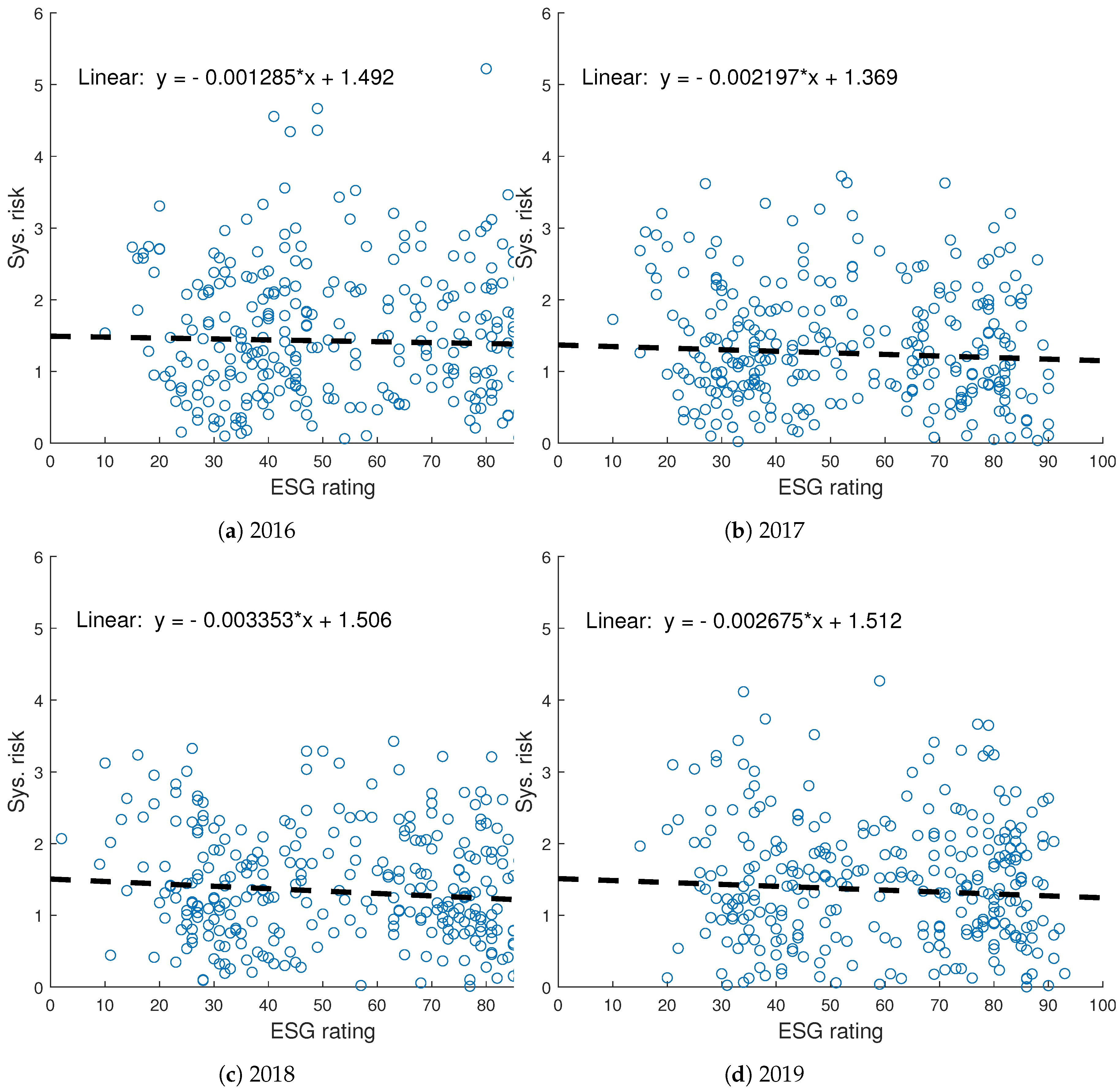
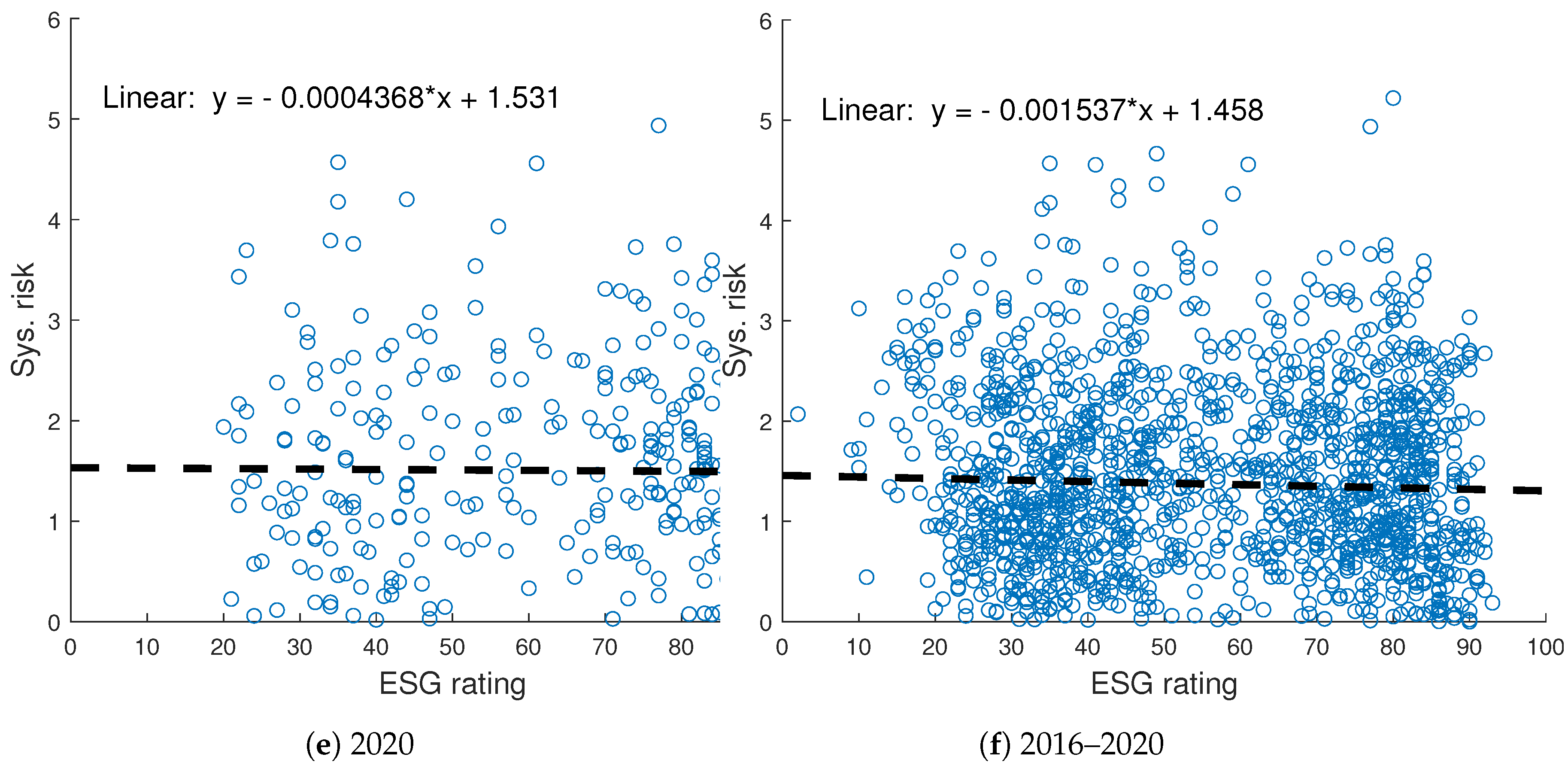
5.3. Systemic Risk and ESG Ratings
5.3.1. Fixed Effects Regressions
5.3.2. OLS Regressions for 2020
5.3.3. Further Regressions
6. Conclusions
Author Contributions
Funding
Institutional Review Board Statement
Informed Consent Statement
Data Availability Statement
Acknowledgments
Conflicts of Interest
Appendix A
Appendix A.1. Tables and Figures

| Stock Names | Countries | Industry | Average ESG Rating |
|---|---|---|---|
| Unilever NV | United Kingdom | Personal products | 89.6 |
| Koninklijke KPN NV | Netherlands | Telecommunication services | 89.4 |
| CNH Industrial NV | United Kingdom | Machinery and Electrical Equipment | 88.8 |
| Red Electrica Corporacion SA | Spain | Electric utilities | 88.8 |
| Energias de Portugal SA | Portugal | Electric utilities | 88.6 |
| Iberdrola SA | Spain | Electric utilities | 88.2 |
| Roche Hldgs AG Ptg Genus | Switzerland | Pharmaceuticals | 88.2 |
| Banco Santander SA | Spain | Banks | 87.2 |
| UPM-Kymmene Oyj | Finland | Paper and forest products | 87.2 |
| Allianz SE | Germany | Insurance | 87 |
| Enagas SA | Spain | Gas utilities | 86.8 |
| Enel SpA | Italy | Electric utilities | 86.6 |
| GlaxoSmithKline | United Kingdom | Pharmaceuticals | 86.2 |
| Telecom Italia SpA | Italy | Telecommunication services | 86.2 |
| Diageo Plc | United Kingdom | Beverages | 86 |
| Endesa SA | Spain | Electric utilities | 85.4 |
| Deutsche Telekom AG | Germany | Telecommunication services | 85.2 |
| Koninklijke Philips Electronics NV | Netherlands | Health Care Equipment & Supplies | 84.6 |
| Naturgy Energy Group SA | Spain | Gas utilities | 84.6 |
| UBS Group AG | Switzerland | Diversified Financial Services and Capital Markets | 84.6 |
| Clariant AG Reg | Switzerland | Chemicals | 84.4 |
| Lanxess AG | Germany | Chemicals | 84.4 |
| Schneider Electric SE | France | Electrical Components and Equipment | 84.2 |
| Adidas AG | Germany | Textiles, Apparel & Luxury Goods | 84 |
| CaixaBank | Spain | Banks | 84 |
| Stock Tickers | Countries | Net EC | Abs. EC. | Abs. CC. | Sys.Rk. | ESG |
|---|---|---|---|---|---|---|
| BNP Paribas | France | 0.1028 | 0.0558 | 0.063 | 6.4293 | 81 |
| Investor AB B | Sweden | 0.0993 | 0.0588 | 0.0631 | 1.3355 | 40 |
| Societe Generale | France | 0.0965 | 0.061 | 0.0645 | 13.708 | 79 |
| Banco Santander SA | Spain | 0.0962 | 0.053 | 0.0629 | 9.4054 | 83 |
| Allianz SE | Germany | 0.0954 | 0.0583 | 0.0644 | 1.6231 | 87 |
| Swiss Life Reg | Switzerland | 0.0938 | 0.0578 | 0.0629 | 1.5106 | 51 |
| Credit Agricole SA | France | 0.0937 | 0.0568 | 0.062 | 9.2656 | 46 |
| BASF SE | Germany | 0.0926 | 0.0569 | 0.0631 | 2.806 | 37 |
| Banco Bilbao V.A. SA | Spain | 0.0899 | 0.0623 | 0.0659 | 9.592 | 87 |
| Zurich Insurance Gr. AG | Switzerland | 0.0898 | 0.0595 | 0.0627 | 1.3731 | 90 |
| Industrivarden AB A | Sweden | 0.0886 | 0.0527 | 0.0597 | 1.3141 | 30 |
| Daimler AG | Germany | 0.0881 | 0.0537 | 0.0603 | 4.59 | 25 |
| ING Groep NV | Netherlands | 0.0877 | 0.0572 | 0.062 | 6.3443 | 52 |
| Porsche Automobil H. SE | Germany | 0.0873 | 0.0518 | 0.059 | 8.0125 | 19 |
| AXA | France | 0.0865 | 0.0569 | 0.0625 | 3.1282 | 88 |
| Bayer Motoren Werke AG | Germany | 0.0861 | 0.0546 | 0.0601 | 3.6705 | 80 |
| Sandvik AB | Sweden | 0.0857 | 0.0573 | 0.0626 | 5.4072 | 76 |
| Credit Suisse Group AG | Switzerland | 0.0857 | 0.057 | 0.0643 | 10.308 | 65 |
| TOTAL SA | France | 0.0854 | 0.0565 | 0.06 | 2.7486 | 75 |
| UBS Group AG | Switzerland | 0.0836 | 0.0542 | 0.062 | 4.7065 | 84 |
| Volkswagen AG | Germany | 0.0832 | 0.0546 | 0.0593 | 5.4902 | 62 |
| Repsol SA | Spain | 0.0831 | 0.0584 | 0.0618 | 7.0166 | 38 |
| SEB-Skand Enskilda B. A | Sweden | 0.0827 | 0.0569 | 0.0628 | 2.7802 | 48 |
| LVMH-Moet Vuitton | France | 0.0826 | 0.057 | 0.0639 | 3.8778 | 69 |
| BHP Group Plc | United Kingdom | 0.0825 | 0.0576 | 0.0626 | 17.8649 | 43 |
| Stock Tickers | Countries | Net EC | Abs. EC. | Abs. CC. | Sys.Rk. | ESG |
|---|---|---|---|---|---|---|
| BNP Paribas | France | 0.1008 | 0.0559 | 0.0633 | 12.4525 | 81 |
| Investor AB B | Sweden | 0.0977 | 0.0584 | 0.0632 | 1.7187 | 40 |
| Societe Generale | France | 0.0956 | 0.0615 | 0.065 | 31.57 | 79 |
| Swiss Life Reg | Switzerland | 0.0944 | 0.0565 | 0.0624 | 3.4205 | 51 |
| Credit Agricole SA | France | 0.0938 | 0.0563 | 0.0616 | 13.335 | 46 |
| Banco Santander SA | Spain | 0.0932 | 0.0534 | 0.0632 | 14.4758 | 83 |
| Allianz SE | Germany | 0.093 | 0.0573 | 0.0637 | 2.5602 | 87 |
| BASF SE | Germany | 0.0924 | 0.0567 | 0.063 | 4.5193 | 37 |
| Banco Bilbao V.A. SA | Spain | 0.0909 | 0.0625 | 0.0661 | 16.1662 | 87 |
| Zurich Insurance Gr. AG | Switzerland | 0.0889 | 0.0594 | 0.0629 | 2.7679 | 90 |
| Daimler AG | Germany | 0.0882 | 0.0534 | 0.0599 | 15.4757 | 25 |
| Industrivarden AB A | Sweden | 0.0873 | 0.0517 | 0.0596 | 1.7714 | 30 |
| BHP Group Plc | United Kingdom | 0.087 | 0.0577 | 0.0625 | 16.0257 | 43 |
| Porsche Automobil H. SE | Germany | 0.0869 | 0.0512 | 0.0591 | 6.9316 | 19 |
| BP Plc | United Kingdom | 0.0864 | 0.0541 | 0.0606 | 11.6752 | 48 |
| ING Groep NV | Netherlands | 0.0858 | 0.0568 | 0.0621 | 12.3155 | 52 |
| Sandvik AB | Sweden | 0.0856 | 0.0574 | 0.0628 | 7.1167 | 76 |
| Bayer Motoren Werke AG | Germany | 0.0855 | 0.0548 | 0.06 | 4.8539 | 80 |
| Credit Suisse Group AG | Switzerland | 0.0853 | 0.0566 | 0.064 | 9.406 | 65 |
| Royal Dutch Shell Plc | Netherlands | 0.0838 | 0.052 | 0.0606 | 10.135 | 68 |
| TOTAL SA | France | 0.0832 | 0.0572 | 0.0599 | 3.9101 | 75 |
| AXA | France | 0.0831 | 0.0575 | 0.0624 | 4.705 | 88 |
| UBS Group AG | Switzerland | 0.0828 | 0.0536 | 0.0615 | 5.3577 | 84 |
| Siemens AG | Germany | 0.0826 | 0.0525 | 0.0585 | 3.2297 | 81 |
| Repsol SA | Spain | 0.0825 | 0.0577 | 0.0615 | 11.8172 | 38 |
| Stock Tickers | Countries | Net EC | Abs. EC. | Abs. CC. | Sys.Rk. | ESG |
|---|---|---|---|---|---|---|
| Unilever NV | United Kingdom | 0.0365 | 0.0527 | 0.0591 | 1.0489 | 91 |
| Telecom Italia SpA | Italy | 0.0406 | 0.0501 | 0.0565 | 15.1736 | 90 |
| Zurich Insurance Gr. AG | Switzerland | 0.0898 | 0.0595 | 0.0627 | 1.3731 | 90 |
| CNH Industrial NV | United Kingdom | 0.0551 | 0.0534 | 0.0595 | 13.8615 | 89 |
| Deutsche Telekom AG | Germany | 0.0544 | 0.0556 | 0.059 | 0.9918 | 89 |
| Enel SpA | Italy | 0.0603 | 0.0556 | 0.0605 | 1.9888 | 89 |
| Koninklijke KPN NV | Netherlands | 0.0331 | 0.0552 | 0.0603 | 2.4549 | 89 |
| Red Electrica Corp. SA | Spain | 0.0367 | 0.0541 | 0.06 | 1.1784 | 89 |
| Roche Hldgs AG Ptg Gen. | Switzerland | 0.0435 | 0.0531 | 0.0595 | 0.7459 | 89 |
| AXA | France | 0.0865 | 0.0569 | 0.0625 | 3.1282 | 88 |
| Energias de Portugal SA | Portugal | 0.0336 | 0.0551 | 0.059 | 1.8833 | 88 |
| GlaxoSmithKline | United Kingdom | 0.0344 | 0.0531 | 0.0592 | 1.2531 | 88 |
| Schneider Electric SE | France | 0.0795 | 0.0551 | 0.0621 | 3.5495 | 88 |
| UPM-Kymmene Oyj | Finland | 0.0598 | 0.06 | 0.0653 | 4.1734 | 88 |
| Allianz SE | Germany | 0.0954 | 0.0583 | 0.0644 | 1.6231 | 87 |
| Banco Bilbao V.A. SA | Spain | 0.0899 | 0.0623 | 0.0659 | 9.592 | 87 |
| Burberry Group | United Kingdom | 0.0417 | 0.0606 | 0.0622 | 8.5782 | 87 |
| Diageo Plc | United Kingdom | 0.0438 | 0.0613 | 0.0644 | 1.0848 | 87 |
| Enagas SA | Spain | 0.0393 | 0.0525 | 0.0601 | 2.2418 | 87 |
| Endesa SA | Spain | 0.0399 | 0.0542 | 0.0614 | 1.1404 | 87 |
| Lanxess AG | Germany | 0.0729 | 0.0532 | 0.0594 | 7.9381 | 87 |
| Moncler SpA | Italy | 0.0449 | 0.0586 | 0.0613 | 8.3403 | 87 |
| Swiss Re Reg | Switzerland | 0.0753 | 0.0518 | 0.0609 | 1.5014 | 87 |
| Iberdrola SA | Spain | 0.0511 | 0.0559 | 0.0607 | 1.2038 | 86 |
| Naturgy Energy Gr. SA | Spain | 0.0449 | 0.0566 | 0.0618 | 1.7394 | 86 |
| Stock Tickers | Countries | Net EC | Abs. EC. | Abs. CC. | Sys.Rk. | ESG |
|---|---|---|---|---|---|---|
| Unilever NV | United Kingdom | 0.0363 | 0.0512 | 0.0583 | 0.6753 | 91 |
| Telecom Italia SpA | Italy | 0.0409 | 0.0501 | 0.0561 | 14.4551 | 90 |
| Zurich Insurance Gr. AG | Switzerland | 0.0889 | 0.0594 | 0.0629 | 2.7679 | 90 |
| CNH Industrial NV | United Kingdom | 0.0536 | 0.0527 | 0.0589 | 14.949 | 89 |
| Deutsche Telekom AG | Germany | 0.0524 | 0.0562 | 0.0593 | 0.9406 | 89 |
| Enel SpA | Italy | 0.0618 | 0.0549 | 0.0598 | 1.91 | 89 |
| Koninklijke KPN NV | Netherlands | 0.0327 | 0.0551 | 0.0605 | 1.583 | 89 |
| Red Electrica Corp. SA | Spain | 0.0389 | 0.0541 | 0.06 | 0.9985 | 89 |
| Roche Hldgs AG Ptg Gen. | Switzerland | 0.0429 | 0.0524 | 0.0591 | 0.7583 | 89 |
| AXA | France | 0.0831 | 0.0575 | 0.0624 | 4.705 | 88 |
| Energias de Portugal SA | Portugal | 0.0313 | 0.0557 | 0.0594 | 1.9214 | 88 |
| GlaxoSmithKline | United Kingdom | 0.035 | 0.0536 | 0.0593 | 1.0876 | 88 |
| Schneider Electric SE | France | 0.0786 | 0.0557 | 0.0619 | 3.7223 | 88 |
| UPM-Kymmene Oyj | Finland | 0.0567 | 0.06 | 0.0648 | 2.8815 | 88 |
| Allianz SE | Germany | 0.093 | 0.0573 | 0.0637 | 2.5602 | 87 |
| Banco Bilbao V.A. SA | Spain | 0.0909 | 0.0625 | 0.0661 | 16.1662 | 87 |
| Burberry Group | United Kingdom | 0.043 | 0.0609 | 0.0626 | 8.7603 | 87 |
| Diageo Plc | United Kingdom | 0.0476 | 0.0626 | 0.065 | 1.0954 | 87 |
| Enagas SA | Spain | 0.0413 | 0.0537 | 0.0602 | 2.6524 | 87 |
| Endesa SA | Spain | 0.0422 | 0.0534 | 0.0609 | 0.994 | 87 |
| Lanxess AG | Germany | 0.0718 | 0.0532 | 0.0595 | 6.8079 | 87 |
| Moncler SpA | Italy | 0.0452 | 0.0584 | 0.0609 | 7.5916 | 87 |
| Swiss Re Reg | Switzerland | 0.0765 | 0.0515 | 0.0608 | 3.1312 | 87 |
| Iberdrola SA | Spain | 0.0538 | 0.0562 | 0.0605 | 1.5353 | 86 |
| Naturgy Energy Gr. SA | Spain | 0.0465 | 0.0567 | 0.0619 | 1.5673 | 86 |
| Stock Tickers | Countries | Net EC | Abs. EC. | Abs. CC. | Sys.Rk. | ESG |
|---|---|---|---|---|---|---|
| Wirecard AG | Germany | 0.0178 | 0.0537 | 0.0585 | 87.3601 | 11 |
| Anglo American Plc | United Kingdom | 0.063 | 0.0556 | 0.0623 | 69.7374 | 80 |
| ArcelorMittal Inc | Luxembourg | 0.0643 | 0.0525 | 0.0591 | 61.4661 | 49 |
| Bank of Ireland Group | Ireland | 0.0415 | 0.054 | 0.0577 | 50.872 | 44 |
| Glencore Plc | Switzerland | 0.0603 | 0.0539 | 0.0599 | 42.5701 | 41 |
| Unicredit SpA Ord | Italy | 0.0587 | 0.053 | 0.0601 | 42.048 | 49 |
| Deutsche Bank AG | Germany | 0.0509 | 0.0529 | 0.0599 | 28.2856 | 56 |
| Commerzbank AG | Germany | 0.0665 | 0.054 | 0.0583 | 26.2122 | 39 |
| STMicroelectronics NV | Switzerland | 0.0573 | 0.0544 | 0.0609 | 23.7928 | 80 |
| ThyssenKrupp AG | Germany | 0.054 | 0.0529 | 0.0604 | 23.2879 | 20 |
| Banco de Sabadell SA | Spain | 0.0558 | 0.0538 | 0.0621 | 21.9302 | 55 |
| Easyjet | United Kingdom | 0.0391 | 0.0578 | 0.0631 | 21.8589 | 18 |
| TUI AG | Germany | 0.0435 | 0.062 | 0.0645 | 21.8324 | 65 |
| Pandora A/S | Denmark | 0.0231 | 0.0526 | 0.056 | 20.5019 | 20 |
| Valeo | France | 0.0584 | 0.0521 | 0.0578 | 20.1379 | 76 |
| Melrose Industries Plc | United Kingdom | 0.0463 | 0.0502 | 0.0574 | 19.8368 | 15 |
| Weir Group | United Kingdom | 0.0609 | 0.0591 | 0.0615 | 19.52 | 36 |
| Micro Focus International | United Kingdom | 0.0327 | 0.05 | 0.0563 | 19.4467 | 17 |
| GVC Holdings Plc | United Kingdom | 0.0278 | 0.0542 | 0.0601 | 18.8734 | 63 |
| BHP Group Plc | United Kingdom | 0.0825 | 0.0576 | 0.0626 | 17.8649 | 43 |
| Electricite de France | France | 0.0377 | 0.0534 | 0.0586 | 17.538 | 84 |
| Inter. Cons. A. Gr. SA | Spain | 0.0522 | 0.0568 | 0.0619 | 16.8167 | 32 |
| Mediobanca SpA | Italy | 0.0628 | 0.053 | 0.0589 | 15.1757 | 53 |
| Telecom Italia SpA | Italy | 0.0406 | 0.0501 | 0.0565 | 15.1736 | 90 |
| Ryanair Holdings Plc | Ireland | 0.0348 | 0.0493 | 0.0577 | 15.0289 | 17 |
| Stock Tickers | Countries | Net EC | Abs. EC. | Abs. CC. | Sys.Rk. | ESG |
|---|---|---|---|---|---|---|
| Wirecard AG | Germany | 0.0173 | 0.0551 | 0.0592 | 1050.2487 | 11 |
| TUI AG | Germany | 0.0445 | 0.0629 | 0.0648 | 138.6509 | 65 |
| Bank of Ireland Group | Ireland | 0.0424 | 0.0541 | 0.0576 | 96.2661 | 44 |
| Carnival Plc | United Kingdom | 0.0477 | 0.0534 | 0.0582 | 95.1087 | 47 |
| ArcelorMittal Inc | Luxembourg | 0.0647 | 0.0515 | 0.0587 | 66.7692 | 49 |
| Inter. Cons. A. Gr. SA | Spain | 0.0543 | 0.0573 | 0.0622 | 64.9675 | 32 |
| Unibail Rodamco Westfield | France | 0.0662 | 0.0565 | 0.0611 | 50.7264 | 41 |
| ThyssenKrupp AG | Germany | 0.0536 | 0.0531 | 0.0599 | 44.1727 | 20 |
| Easyjet | United Kingdom | 0.0407 | 0.0569 | 0.0632 | 42.9224 | 18 |
| Rolls-Royce Holdings Plc | United Kingdom | 0.0425 | 0.0547 | 0.0588 | 42.6259 | 74 |
| Renault SA | France | 0.0625 | 0.0549 | 0.0596 | 41.3718 | 45 |
| Melrose Industries Plc | United Kingdom | 0.0477 | 0.05 | 0.0578 | 40.107 | 15 |
| Anglo American Plc | United Kingdom | 0.0668 | 0.0557 | 0.0622 | 36.328 | 80 |
| Commerzbank AG | Germany | 0.0669 | 0.0545 | 0.0586 | 34.3686 | 39 |
| Societe Generale | France | 0.0956 | 0.0615 | 0.065 | 31.57 | 79 |
| Micro Focus International | United Kingdom | 0.0345 | 0.0505 | 0.0559 | 30.9013 | 17 |
| Valeo | France | 0.0568 | 0.0522 | 0.057 | 30.5707 | 76 |
| Klepierre | France | 0.0594 | 0.0581 | 0.0623 | 28.5112 | 40 |
| Banco de Sabadell SA | Spain | 0.0555 | 0.0546 | 0.0625 | 27.3305 | 55 |
| Glencore Plc | Switzerland | 0.0632 | 0.0532 | 0.0595 | 26.7761 | 41 |
| Deutsche Bank AG | Germany | 0.0509 | 0.0534 | 0.06 | 25.4111 | 56 |
| GVC Holdings Plc | United Kingdom | 0.0293 | 0.0539 | 0.06 | 23.5431 | 63 |
| ABN AMRO Group NV | Netherlands | 0.0577 | 0.0504 | 0.0593 | 22.6387 | 83 |
| Ryanair Holdings Plc | Ireland | 0.0362 | 0.0485 | 0.0573 | 22.2129 | 17 |
| Unicredit SpA Ord | Italy | 0.0579 | 0.052 | 0.0594 | 22.0486 | 49 |
| Stock Tickers | Countries | Net EC | Abs. EC. | Abs. CC. | Sys.Rk. | ESG |
|---|---|---|---|---|---|---|
| Swiss Prime Site AG | Switzerland | 0.031 | 0.0556 | 0.0612 | 0.3777 | 25 |
| Swisscom AG Reg | Switzerland | 0.0521 | 0.0539 | 0.0588 | 0.4423 | 58 |
| Nestle SA Reg | Switzerland | 0.0456 | 0.054 | 0.0578 | 0.4996 | 72 |
| Beiersdorf AG | Germany | 0.0438 | 0.054 | 0.0617 | 0.7235 | 29 |
| Roche Hldgs AG Ptg Gen. | Switzerland | 0.0435 | 0.0531 | 0.0595 | 0.7459 | 89 |
| SGS-Soc Gen Surveil Hldg R. | Switzerland | 0.0573 | 0.0521 | 0.0571 | 0.7497 | 85 |
| Groupe Bruxelles Lambert | Belgium | 0.0822 | 0.0508 | 0.0581 | 0.7744 | 38 |
| Geberit AG Reg | Switzerland | 0.0636 | 0.0556 | 0.0594 | 0.7797 | 37 |
| Givaudan AG | Switzerland | 0.0475 | 0.0526 | 0.0613 | 0.8175 | 37 |
| Lindt & Sprungli AG R. | Switzerland | 0.0324 | 0.0554 | 0.0584 | 0.8263 | 23 |
| Heineken NV | Netherlands | 0.0558 | 0.0581 | 0.0631 | 0.8693 | 82 |
| Orkla AS | Norway | 0.0222 | 0.0566 | 0.0605 | 0.9364 | 62 |
| Novartis AG Reg | Switzerland | 0.0506 | 0.0541 | 0.0593 | 0.945 | 73 |
| Kuehne & Nagel Intl. AG R. | Switzerland | 0.0466 | 0.0594 | 0.063 | 0.9477 | 48 |
| Carlsberg AS B | Denmark | 0.035 | 0.0543 | 0.0608 | 0.9688 | 24 |
| Henkel AG & Co. K. N. P. | Germany | 0.0464 | 0.0562 | 0.0597 | 0.9768 | 37 |
| Partners Group Hldg | Switzerland | 0.0552 | 0.0594 | 0.0628 | 0.9828 | 55 |
| Danone | France | 0.0468 | 0.0584 | 0.0609 | 0.991 | 69 |
| Deutsche Telekom AG | Germany | 0.0544 | 0.0556 | 0.059 | 0.9918 | 89 |
| Unilever NV | United Kingdom | 0.0365 | 0.0527 | 0.0591 | 1.0489 | 91 |
| Telia Company AB | Sweden | 0.0485 | 0.0528 | 0.0592 | 1.0531 | 32 |
| Diageo Plc | United Kingdom | 0.0438 | 0.0613 | 0.0644 | 1.0848 | 87 |
| Pernod-Ricard | France | 0.0472 | 0.0575 | 0.0623 | 1.0926 | 34 |
| SEGRO Plc | United Kingdom | 0.041 | 0.0515 | 0.0609 | 1.1128 | 58 |
| Endesa SA | Spain | 0.0399 | 0.0542 | 0.0614 | 1.1404 | 87 |
| Stock Tickers | Countries | Net EC | Abs. EC. | Abs. CC. | Sys.Rk. | ESG |
|---|---|---|---|---|---|---|
| Nestle SA Reg | Switzerland | 0.0451 | 0.054 | 0.0575 | 0.3749 | 72 |
| Swisscom AG Reg | Switzerland | 0.0502 | 0.0543 | 0.0593 | 0.4261 | 58 |
| Swiss Prime Site AG | Switzerland | 0.0286 | 0.0558 | 0.0616 | 0.555 | 25 |
| Beiersdorf AG | Germany | 0.0447 | 0.053 | 0.0616 | 0.6034 | 29 |
| SGS-Soc Gen Surveil Hldg R. | Switzerland | 0.0549 | 0.0536 | 0.0573 | 0.6687 | 85 |
| Unilever NV | United Kingdom | 0.0363 | 0.0512 | 0.0583 | 0.6753 | 91 |
| Givaudan AG | Switzerland | 0.047 | 0.0515 | 0.061 | 0.6793 | 37 |
| Lindt & Sprungli AG R. | Switzerland | 0.0326 | 0.0552 | 0.0589 | 0.709 | 23 |
| Novartis AG Reg | Switzerland | 0.0494 | 0.0534 | 0.0591 | 0.7266 | 73 |
| Roche Hldgs AG Ptg Gen. | Switzerland | 0.0429 | 0.0524 | 0.0591 | 0.7583 | 89 |
| Telia Company AB | Sweden | 0.0472 | 0.0528 | 0.0588 | 0.7846 | 32 |
| Danone | France | 0.0458 | 0.0587 | 0.0611 | 0.7928 | 69 |
| Orkla AS | Norway | 0.022 | 0.0572 | 0.0601 | 0.8446 | 62 |
| Schindler-Hldg AG Reg | Switzerland | 0.0458 | 0.054 | 0.0604 | 0.9048 | 26 |
| Henkel AG & Co. K. N. P. | Germany | 0.0484 | 0.0566 | 0.0598 | 0.9162 | 37 |
| Deutsche Wohnen AG BR | Germany | 0.0291 | 0.0559 | 0.0613 | 0.9172 | 27 |
| Deutsche Telekom AG | Germany | 0.0524 | 0.0562 | 0.0593 | 0.9406 | 89 |
| Ahold Delhaize NV | Netherlands | 0.0259 | 0.0571 | 0.0613 | 0.9408 | 83 |
| Geberit AG Reg | Switzerland | 0.0605 | 0.057 | 0.06 | 0.9641 | 37 |
| Endesa SA | Spain | 0.0422 | 0.0534 | 0.0609 | 0.994 | 87 |
| Kuehne & Nagel Intl. AG R. | Switzerland | 0.0449 | 0.0597 | 0.063 | 0.9956 | 48 |
| Red Electrica Corp. SA | Spain | 0.0389 | 0.0541 | 0.06 | 0.9985 | 89 |
| Elisa Corporation | Finland | 0.0288 | 0.0536 | 0.0589 | 1.0182 | 31 |
| Wolters Kluwer NV | Netherlands | 0.0436 | 0.0518 | 0.0579 | 1.0284 | 30 |
| Croda Intl | United Kingdom | 0.0399 | 0.0554 | 0.0616 | 1.031 | 35 |

Appendix A.2. Tables Related to Stock Data
| ISO | Industry | Model | |||
|---|---|---|---|---|---|
| Ticker | Company | Market Cap in Billion $ | Code | Code | Inclusion |
| 1COV.DE | Covestro AG | 7585 | DE | CHM | ooo |
| AAL.L | Anglo American PLC | 35,532 | GB | MNX | ooo |
| ABBN.SW | ABB Ltd | 46,631 | CH | ELQ | oo |
| ABF.L | Associated British Foods | 24,306 | GB | FOA | ooo |
| ABI.BR | Anheuser Busch Inbev NV | 123,000 | BE | BVG | ooo |
| ABN.AS | ABN AMRO Group NV | 15,246 | NL | BNK | oo |
| AC.PA | Accor | 11,274 | FR | TRT | ooo |
| ACA.PA | Credit Agricole SA | 37,284 | FR | BNK | oo |
| ACS.MC | ACS Actividades de | 11,217 | ES | CON | ooo |
| Construccion y Servicios SA | |||||
| AD.AS | Ahold Delhaize NV | 26,391 | NL | FDR | oo |
| ADP.PA | ADP Promesses | 17,427 | FR | PRO | o |
| ADS.DE | Adidas AG | 58,080 | DE | TEX | ooo |
| AENA.MC | Aena SA | 25,575 | ES | TRA | ooo |
| AGN.AS | Aegon NV | 8523 | NL | INS | oo |
| AGS.BR | AGEAS | 10,450 | BE | INS | oo |
| AHT.L | Ashtead Group | 14,359 | GB | TCD | ooo |
| AI.PA | L’Air Liquide S.A. | 59,445 | FR | CHM | ooo |
| AIR.PA | Airbus SE | 101,000 | FR | ARO | ooo |
| AKE.PA | Arkema | 7242 | FR | CHM | ooo |
| AKZA.AS | Akzo Nobel NV | 20,643 | NL | CHM | ooo |
| ALFA.ST | Alfa Laval AB | 9490 | SE | IEQ | ooo |
| ALO.PA | Alstom | 9472 | FR | IEQ | ooo |
| ALV.DE | Allianz SE | 91,110 | DE | INS | oo |
| AMS.MC | Amadeus IT Group SA | 31,396 | ES | TSV | ooo |
| ASML.AS | ASML Holding NV | 112,000 | NL | SEM | ooo |
| ASSA-B.ST | Assa Abloy B | 22,025 | SE | BLD | oo |
| ATCO-A.ST | Atlas Copco AB A | 29,893 | SE | IEQ | oo |
| ATL.MI | Atlantia SpA | 17,153 | IT | TRA | ooo |
| ATO.PA | AtoS SE | 8115 | FR | TSV | ooo |
| AV.L | Aviva | 19,478 | GB | INS | oo |
| AZN.L | AstraZeneca PLC | 118,000 | GB | DRG | ooo |
| BA.L | BAE Systems PLC | 23,152 | GB | ARO | ooo |
| BAER.SW | Julius Baer Group | 10,284 | CH | FBN | oo |
| BALN.SW | Baloise Hldg Reg | 7859 | CH | INS | o |
| BARC.L | Barclays | 36,376 | GB | BNK | oo |
| BAS.DE | BASF SE | 61,859 | DE | CHM | ooo |
| BATS.L | British American | 94,014 | GB | TOB | oo |
| BAYN.DE | Bayer AG | 67,899 | DE | DRG | oo |
| BBVA.MC | Banco Bilbao Vizcaya | 33,226 | ES | BNK | oo |
| Argentaria SA |
| ISO | Industry | Model | |||
|---|---|---|---|---|---|
| Ticker | Company | Market Cap in Billion $ | Code | Code | Inclusion |
| BDEV.L | Barratt Developments | 8981 | GB | HOM | ooo |
| Tobacco PLC | |||||
| BEI.DE | Beiersdorf AG | 26,875 | DE | COS | ooo |
| BHP.L | BHP Group Plc | 44,349 | GB | MNX | ooo |
| BIRG.IR | Bank of Ireland Group | 5270 | IE | BNK | oo |
| BKG.L | Berkeley Group | 7860 | GB | HOM | ooo |
| Holdings Plc | |||||
| BLND.L | British Land Co | 7108 | GB | REA | oo |
| BMW.DE | Bayer Motoren Werke | 44,029 | DE | AUT | oo |
| AG (BMW) | |||||
| BN.PA | danone | 50,625 | FR | FOA | ooo |
| BNP.PA | BNP Paribas | 65,744 | FR | BNK | oo |
| BNR.DE | Brenntag AG | 7490 | DE | TCD | ooo |
| BNZL.L | Bunzl | 8190 | GB | TCD | ooo |
| BOL.ST | Boliden AB | 6478 | SE | MNX | ooo |
| BP.L | BP p.l.c | 120,000 | GB | OGX | ooo |
| BRBY.L | Burberry Group | 10,719 | GB | TEX | ooo |
| BT-A.L | BT Group | 22,669 | GB | TLS | ooo |
| BVI.PA | Bureau Veritas SA | 10,512 | FR | PRO | oo |
| CA.PA | Carrefour SA | 12,068 | FR | FDR | oo |
| CABK.MC | CaixaBank | 16,736 | ES | BNK | oo |
| CAP.PA | Capgemini SE | 18,218 | FR | TSV | ooo |
| CARL-B.CO | Carlsberg AS B | 15,807 | DK | BVG | ooo |
| CBK.DE | Commerzbank AG | 6909 | DE | BNK | oo |
| CCL.L | Carnival Plc | 9321 | GB | TRT | oo |
| CFR.SW | Richemont, Cie | 36,538 | CH | TEX | oo |
| Financiere A Br | |||||
| CHR.CO | Christian Hansen Holding A/S | 9341 | DK | LIF | oo |
| CLN.SW | Clariant AG Reg | 6598 | CH | CHM | ooo |
| CLNX.MC | Cellnex Telecom S.A. | 14,784 | ES | TLS | o |
| CNA.L | Centrica | 6152 | GB | MUW | ooo |
| CNHI.MI | CNH Industrial NV | 13,325 | IT | IEQ | oo |
| COLO-B.CO | Coloplast AS B | 21,897 | DK | HEA | ooo |
| CON.DE | Continental AG | 23,052 | DE | ATX | ooo |
| CPG.L | Compass Group | 35,582 | GB | REX | ooo |
| CRDA.L | Croda Intl | 7981 | GB | CHM | ooo |
| CRH | CRH Plc | 28,198 | IE | COM | ooo |
| CS.PA | AXA | 60,928 | FR | INS | oo |
| CSGN.SW | Credit Suisse Group AG | 30,826 | CH | FBN | oo |
| DAI.DE | Daimler AG | 52,817 | DE | AUT | ooo |
| DANSKE.CO | Danske Bank A/S | 12,437 | DK | BNK | oo |
| DASTY | Dassault Systemes SA | 38,532 | FR | SOF | ooo |
| DB | Deutsche Bank AG | 14,295 | DE | BNK | oo |
| DB1.DE | Deutsche Boerse AG | 26,628 | DE | FBN | oo |
| ISO | Industry | Model | |||
|---|---|---|---|---|---|
| Ticker | Company | Market Cap in Billion $ | Code | Code | Inclusion |
| DCC.L | DCC | 7836 | IE | IDD | ooo |
| DG.PA | Vinci | 59,918 | FR | CON | ooo |
| DGE.L | Diageo Plc | 97,310 | GB | BVG | ooo |
| DLG.L | Direct Line Insurance | 5078 | GB | INS | oo |
| Group | |||||
| DNB.OL | DNB ASA | 26,283 | NO | BNK | oo |
| DPW.DE | Deutsche Post AG | 41,805 | DE | TRA | ooo |
| DSM.AS | Koninklijke DSM NV | 21,063 | NL | CHM | ooo |
| DSV.CO | Dsv Panalpina A/s | 24,146 | DK | TRA | ooo |
| DTE.DE | Deutsche Telekom AG | 69,374 | DE | TLS | oo |
| DWNI.DE | Deutsche Wohnen AG BR | 13,100 | DE | REA | oo |
| EBS.VI | Erste Group Bank AG | 14,424 | AT | BNK | oo |
| EDEN.PA | Edenred | 11,211 | FR | TSV | ooo |
| EDF.PA | Electricite de France | 30,290 | FR | ELC | ooo |
| EDP.LS | Energias de Portugal SA | 11,931 | PT | ELC | oo |
| EL.PA | EssilorLuxottica | 58,853 | FR | TEX | ooo |
| ELE.MC | Endesa SA | 25,187 | ES | ELC | ooo |
| ELISA.HE | Elisa Corporation | 8190 | FI | TLS | ooo |
| ELUX-B.ST | Electrolux AB B | 6571 | SE | DHP | oo |
| EN.PA | Bouygues | 14,072 | FR | CON | ooo |
| ENEL.MI | Enel SpA | 71,827 | IT | ELC | ooo |
| ENG.MC | Enagas SA | 5428 | ES | GAS | ooo |
| ENGI.PA | Engie | 34,731 | FR | MUW | ooo |
| ENI.MI | ENI SpA | 50,318 | IT | OGX | ooo |
| EOAN.DE | E.ON SE | 25,155 | DE | MUW | ooo |
| EQNR.OL | Equinor ASA | 59,422 | NO | OGX | ooo |
| ERIC-B.ST | Ericsson L.M. Telefonaktie B | 23,660 | SE | CMT | ooo |
| EXO.MI | EXOR NV | 16,648 | IT | FBN | oo |
| EXPN.L | Experian Plc | 29,221 | GB | PRO | oo |
| EZJ.L | Easyjet | 6659 | GB | AIR | ooo |
| FCA.MI | Fiat Chrysler Automobiles NV | 20,446 | IT | AUT | o |
| FER.MC | Ferrovial SA | 19,942 | ES | CON | ooo |
| FERG.L | Ferguson PLC | 18,780 | GB | TCD | ooo |
| FGR.PA | Eiffage | 9996 | FR | CON | ooo |
| FLTR.L | Flutter Entertainment plc | 8465 | IE | CNO | ooo |
| FME.DE | Fresenius Medical Care AG | 20,259 | DE | HEA | ooo |
| FORTUM.HE | Fortum Oyj | 19,544 | FI | ELC | ooo |
| FP.PA | TOTAL SA | 131,000 | FR | OGX | ooo |
| FR.PA | Valeo | 7546 | FR | ATX | ooo |
| G.MI | Assicurazioni Generali SpA | 28,638 | IT | INS | oo |
| G1A.DE | GEA AG | 5320 | DE | IEQ | oo |
| GALP.LS | Galp Energia SGPS SA | 11,490 | PT | OGX | ooo |
| GBLB.BR | Groupe Bruxelles Lambert | 15,161 | BE | FBN | oo |
| GEBN.SW | Geberit AG Reg | 18,517 | CH | BLD | ooo |
| GFC.PA | Gecina | 12,155 | FR | REA | oo |
| ISO | Industry | Model | |||
|---|---|---|---|---|---|
| Ticker | Company | Market Cap in Billion $ | Code | Code | Inclusion |
| GFS.L | G4S Plc | 3997 | GB | ICS | ooo |
| GIVN.SW | Givaudan AG | 25,757 | CH | DRG | ooo |
| GLE.PA | Societe Generale | 26,292 | FR | INS | oo |
| GLEN.L | Glencore Plc | 40,569 | GB | MNX | ooo |
| GLPG.AS | Galapagos Genomics NV | 12,060 | BE | BTC | o |
| GMAB.CO | Genmab AS | 12,880 | DK | BTC | ooo |
| GRF.MC | Grifols SA | 13,393 | ES | BTC | ooo |
| GSK.L | GlaxoSmithKline | 113,000 | GB | DRG | ooo |
| GVC.L | GVC Holdings PLC | 6041 | GB | CNO | oo |
| HEI.DE | HeidelbergCement AG | 12,889 | DE | COM | ooo |
| HEIA.AS | Heineken NV | 54,674 | NL | BVG | ooo |
| HEN3.DE | Henkel AG & Co. KGaA | 16,426 | DE | HOU | ooo |
| Nvtg-Pref | |||||
| HEXA-B.ST | Hexagon AB | 17,520 | SE | ITC | ooo |
| HL.L | Hargreaves Lansdown Plc | 10,846 | GB | FBN | ooo |
| HLMA.L | Halma | 9449 | GB | ITC | ooo |
| HM-B.ST | Hennes & Mauritz AB B | 26,521 | SE | RTS | ooo |
| HNR1.DE | Hannover Ruck SE | 20,778 | DE | INS | oo |
| HO.PA | Thales | 19,586 | FR | ARO | ooo |
| HSBA.L | HSBC Holdings Plc | 144,000 | GB | BNK | oo |
| IAG.L | International Consolidated | 14,713 | GB | AIR | oo |
| Airlines Group SA | |||||
| IMB.L | Imperial Brands PLC | 22,548 | GB | TOB | ooo |
| IMI.L | IMI | 3988 | GB | PRO | o |
| INDU-A.ST | Industrivarden AB A | 5938 | SE | FBN | oo |
| INF.L | Informa PLC | 12,676 | GB | PUB | ooo |
| INGA.AS | ING Groep NV | 41,645 | NL | BNK | oo |
| IBE.MC | Iberdrola SA | 58,403 | ES | ELC | ooo |
| IFX.DE | Infineon Technologies AG | 25,391 | DE | SEM | ooo |
| IHG.L | InterContinental Hotels | 11,553 | GB | TRT | ooo |
| Group PLC | |||||
| III.L | 3I Group | 12,602 | GB | FBN | oo |
| INVE-B.ST | Investor AB B | 22,195 | SE | FBN | oo |
| ISP.MI | Intesa SanPaolo | 41,114 | IT | BNK | oo |
| ITRK.L | Intertek Group PLC | 11,119 | GB | PRO | ooo |
| ITV.L | ITV PLC | 7,183 | GB | PUB | ooo |
| ITX.MC | Inditex SA | 98,018 | ES | RTS | o |
| JMAT.L | Johnson, Matthey | 7,043 | GB | CHM | ooo |
| KBC.BR | KBC Group NV | 27,961 | BE | BNK | oo |
| KER.PA | Kering | 73,803 | FR | TEX | ooo |
| KGP.L | Kingspan Group PLC | 9,888 | IE | BLD | ooo |
| KINV-B.ST | Kinnevik Investment AB B | 5,280 | SE | FBN | oo |
| KNEBV.HE | Kone Corp B | 26,178 | FI | IEQ | oo |
| ISO | Industry | Model | |||
|---|---|---|---|---|---|
| Ticker | Company | Market Cap in Billion $ | Code | Code | Inclusion |
| KNIN.SW | KUEHNE & NAGEL | 18,023 | CH | TRA | ooo |
| INTL AG-REG | |||||
| KPN.AS | Koninklijke KPN NV | 11,057 | NL | TLS | oo |
| KYGA.L | Kerry Group A | 19,531 | IE | FOA | ooo |
| LAND.L | Land Securities Group PLC | 8789 | GB | REA | oo |
| LDO.MI | Leonardo S.p.a. | 6041 | IT | ARO | ooo |
| LEG.DE | LEG Immobilien AG | 7237 | DE | REA | o |
| LGEN.L | Legal & General Group | 21,154 | GB | BNK | oo |
| LHA.DE | Deutsche Lufthansa AG | 7772 | DE | AIR | ooo |
| LHN.SW | LafargeHolcim Ltd | 30,439 | CH | COM | ooo |
| LI.PA | Klepierre | 10,406 | FR | REA | oo |
| LISN.SW | Lindt & Sprungli AG Reg | 10,701 | CH | FOA | oo |
| LLOY.L | Lloyds Banking | 51,831 | GB | BNK | oo |
| Group PLC | |||||
| LOGN.SW | Logitech International SA | 7301 | CH | THQ | ooo |
| LONN.SW | Lonza AG | 24,206 | CH | LIF | oo |
| LR.PA | Legrand Promesses | 19,234 | FR | ELQ | oo |
| LSE.L | London Stock | 32,084 | GB | FBN | oo |
| Exchange PLC | |||||
| LXS.DE | Lanxess AG | 5231 | DE | CHM | ooo |
| MAERSK-A.CO | AP Moller-Maersk AS A | 12,997 | DK | TRA | o |
| MB.MI | Mediobanca SpA | 8648 | IT | BNK | oo |
| MC.PA | LVMH-Moet Vuitton | 211,000 | FR | TEX | ooo |
| MCRO.L | Micro Focus International | 4561 | GB | PRO | ooo |
| MKS.L | Marks & Spencer Group | 4920 | GB | FDR | oo |
| ML.PA | Michelin CGDE B Brown | 19,645 | FR | ATX | oo |
| MNDI.L | Mondi PLC | 10,171 | GB | FRP | ooo |
| MONC.MI | Moncler SpA | 10,336 | IT | TEX | ooo |
| MOWI.OL | Mowi ASA | 11,942 | NO | FOA | ooo |
| MRK.DE | MERCK KGaA | 13,615 | DE | DRG | ooo |
| MRO.L | Melrose Industries PLC | 13,785 | GB | IEQ | ooo |
| MRW.L | Morrison (WM) | 5650 | GB | FDR | ooo |
| Supermarkets | |||||
| MT.AS | ArcelorMittal Inc | 15,888 | LU | STL | ooo |
| MTX.DE | MTU Aero Engines AG | 13,239 | DE | ARO | ooo |
| MUV2.DE | Munich Re AG | 37,955 | DE | INS | o |
| NDA-FI.HE | Nordea Bank Abp | 29,111 | FI | BNK | oo |
| NESN.SW | Nestle SA Reg | 287,000 | CH | FOA | ooo |
| NESTE.HE | Neste Oyj | 23,860 | FI | OGR | ooo |
| NG.L | National Grid PLC | 41,881 | GB | MUW | ooo |
| NHY.OL | Norsk Hydro AS | 6848 | NO | ALU | ooo |
| NN.AS | NN Group N.V. | 11,619 | NL | INS | oo |
| NOKIA.HE | Nokia OYJ | 18,561 | FI | CMT | ooo |
| NOVN.SW | Novartis AG Reg | 216,000 | CH | DRG | ooo |
| NOVO-B.CO | Novo Nordisk AS B | 96,373 | DK | DRG | oo |
| ISO | Industry | Model | |||
|---|---|---|---|---|---|
| Ticker | Company | Market Cap in Billion $ | Code | Code | Inclusion |
| NTGY.MC | Naturgy Energy Group SA | 22,044 | ES | GAS | ooo |
| NXT.L | Next | 11,049 | GB | RTS | ooo |
| NZYM-B.CO | Novozymes AS B | 10,350 | DK | CHM | ooo |
| OCDO.L | Ocado Group PLC | 10,685 | GB | RTS | o |
| OMV.VI | OMV AG | 16,389 | AT | OGX | ooo |
| OR.PA | L’Oreal | 147,000 | FR | COS | ooo |
| ORA.PA | Orange | 34,750 | FR | TLS | ooo |
| ORK.OL | Orkla AS | 9034 | NO | FOA | ooo |
| PAH3.DE | Porsche Automobil | 10,204 | DE | AUT | oo |
| Holding SE | |||||
| PGHN.SW | Partners Group Hldg | 21,805 | CH | REA | ooo |
| PHIA.AS | Koninklijke Philips | 39,397 | NL | MTC | ooo |
| Electronics NV | |||||
| PNDORA.CO | Pandora A/S | 3878 | DK | TEX | ooo |
| PROX.BR | Proximus | 8626 | BE | ELQ | ooo |
| PRU.L | Prudential PLC | 44,280 | GB | INS | oo |
| PRY.MI | Prysmian SpA | 5762 | IT | ELQ | ooo |
| PSN.L | Persimmon | 10,114 | GB | HOM | ooo |
| PSON.L | Pearson | 5876 | GB | PUB | ooo |
| PUB.PA | Publicis Groupe | 9701 | FR | PUB | ooo |
| QIA.DE | QIAGEN NV | 6913 | DE | LIF | ooo |
| RACE.MI | Ferrari NV | 28,681 | IT | AUT | ooo |
| RAND.AS | Randstad NV | 9960 | NL | PRO | oo |
| RB.L | Reckitt Benckiser | 53,348 | GB | HOU | ooo |
| Group PLC | |||||
| RDSA.L | Royal Dutch Shell PLC | 110,000 | GB | OGX | ooo |
| REE.MC | Red Electrica | 9698 | ES | ELC | ooo |
| Corporacion SA | |||||
| REL.L | RELX PLC | 45,300 | GB | PRO | ooo |
| REP.MC | Repsol SA | 22,271 | ES | OGX | ooo |
| RI.PA | Pernod-Ricard | 42,290 | FR | BVG | ooo |
| RIO.L | Rio Tinto PLC | 67,920 | GB | MNX | ooo |
| RMS.PA | Hermes Intl | 70,330 | FR | TEX | o |
| RNO.PA | Renault SA | 12,473 | FR | AUT | oo |
| ROG.SW | Roche Hldgs AG | 203,000 | CH | DRG | ooo |
| Ptg Genus | |||||
| RR.L | Rolls-Royce Holdings PLC | 15,590 | GB | ARO | ooo |
| RSA.L | RSA Insurance Group PLC | 6861 | GB | INS | oo |
| RTO.L | Rentokil Initial | 9836 | GB | ICS | ooo |
| RWE.DE | RWE AG | 16,813 | DE | MUW | oo |
| RY4C.IR | Ryanair Holdings PLC | 15,859 | IE | AIR | ooo |
| SAB.MC | Banco de Sabadell SA | 5840 | ES | BNK | oo |
| SAF.PA | Safran SA | 56,314 | FR | ARO | ooo |
| SAMPO.HE | Sampo Oyj A | 21,562 | FI | INS | oo |
| SAN.MC | Banco Santander SA | 61,985 | ES | BNK | oo |
| ISO | Industry | Model | |||
|---|---|---|---|---|---|
| Ticker | Company | Market Cap in Billion $ | Code | Code | Inclusion |
| SAN.PA | Sanofi-Aventis | 113,000 | FR | DRG | ooo |
| SAND.ST | Sandvik AB | 21,857 | SE | IEQ | ooo |
| SAP.DE | SAP SE | 148,000 | DE | SOF | ooo |
| SBRY.L | Sainsbury (J) | 6008 | GB | FDR | ooo |
| SCA-B.ST | SCA-B shares | 5774 | SE | FRP | o |
| SCHN.SW | Schindler-Hldg AG Reg | 14,642 | CH | IEQ | ooo |
| SCMN.SW | Swisscom AG Reg | 24,437 | CH | TLS | oo |
| SCR.PA | SCOR SE | 6980 | FR | INS | oo |
| SDR.L | Schroders PLC | 8905 | GB | FBN | oo |
| SEB-A.ST | SEB-Skand Enskilda | 18,219 | SE | BNK | oo |
| Banken A | |||||
| SECU-B.ST | Securitas AB B | 5354 | SE | ICS | oo |
| SESG.PA | SES | 4793 | LU | PUB | o |
| SEV.PA | Suez SA | 8406 | FR | MUW | ooo |
| SGE.L | Sage Group | 9912 | GB | SOF | ooo |
| SGO.PA | Saint-Gobain, Cie de | 19,940 | FR | BLD | oo |
| SGRO.L | SEGRO PLC | 11,627 | GB | REA | oo |
| SGSN.SW | SGS-Soc Gen Surveil | 18,624 | CH | PRO | ooo |
| Hldg Reg | |||||
| SHB-A.ST | Svenska Handelsbanken A | 18,699 | SE | BNK | oo |
| SIE.DE | Siemens AG | 99,059 | DE | IDD | ooo |
| SK3.IR | Smurfit Kappa Group PLC | 8096 | IE | CTR | ooo |
| SKA-B.ST | SKANSKA AB-B | 8072 | SE | CON | ooo |
| SKF-B.ST | SKF AB B | 7588 | SE | IEQ | oo |
| SLA.L | Standard Life Aberdeen | 9100 | GB | FBN | oo |
| SLHN.SW | Swiss Life Reg | 15,019 | CH | INS | oo |
| SMDS.L | DS Smith | 6209 | GB | CTR | o |
| SMIN.L | Smiths Group | 7829 | GB | IDD | ooo |
| SN.L | Smith & Nephew | 19,295 | GB | MTC | ooo |
| SOLB.BR | Solvay | 10,936 | BE | CHM | ooo |
| SOON.SW | Sonova Holding AG | 13,127 | CH | MTC | ooo |
| SPSN.SW | Swiss Prime Site AG | 7821 | CH | REA | ooo |
| SPX.L | Spirax-Sarco Engineering | 7724 | GB | IEQ | ooo |
| SREN.SW | Swiss Re Reg | 32,752 | CH | INS | oo |
| SRG.MI | Snam SpA | 15,908 | IT | GAS | ooo |
| SSE.L | Scottish & Southern Energy | 17,583 | GB | ELC | o |
| STAN.L | Standard Chartered | 26,909 | GB | BNK | oo |
| STERV.HE | Stora Enso OYJ R | 7939 | FI | FRP | ooo |
| STJ.L | St James’s Place | 7280 | GB | FBN | oo |
| STM.MI | STMicroelectronics NV | 21,820 | IT | SEM | ooo |
| STMN.SW | Straumann AG Reg | 13,888 | CH | MTC | o |
| SU.PA | Schneider Electric SE | 53,251 | FR | ELQ | ooo |
| SVT.L | Severn Trent | 7138 | GB | MUW | ooo |
| SW.PA | Sodexo | 15,578 | FR | REX | ooo |
| ISO | Industry | Model | |||
|---|---|---|---|---|---|
| Ticker | Company | Market Cap in Billion $ | Code | Code | Inclusion |
| SWED-A.ST | Swedbank AB | 15,047 | SE | BNK | oo |
| SWMA.ST | Swedish Match AB | 7821 | SE | TOB | ooo |
| SY1.DE | Symrise AG | 12,703 | DE | CHM | ooo |
| TATE.L | Tate & Lyle | 4187 | GB | FOA | ooo |
| TEF.MC | Telefonica SA | 32,331 | ES | TLS | ooo |
| TEL.OL | Telenor ASA | 23,032 | NO | TLS | ooo |
| TEL2-B.ST | Tele2 AB B | 8621 | SE | TLS | oo |
| TELIA.ST | Telia Company AB | 16,151 | SE | TLS | ooo |
| TEMN.SW | Temenos Group AG | 10,213 | CH | SOF | o |
| TEN.MI | Tenaris SA | 11,864 | IT | OGX | ooo |
| TEP.PA | Teleperformance | 12,735 | FR | PRO | o |
| TIT.MI | Telecom Italia SpA | 8459 | IT | TLS | ooo |
| TKA.DE | ThyssenKrupp AG | 7495 | DE | IDD | ooo |
| TPK.L | Travis Perkins | 4730 | GB | TCD | ooo |
| TRN.MI | Terna SpA | 11,913 | IT | ELC | o |
| TSCO.L | Tesco | 29,294 | GB | FDR | ooo |
| TUI1.DE | TUI AG | 6612 | DE | TRT | ooo |
| UBI.PA | Ubisoft Entertainment SA | 6939 | FR | IMS | o |
| UBSG.SW | UBS Group AG | 43,098 | CH | FBN | oo |
| UCB.BR | UCB SA | 13,790 | BE | DRG | ooo |
| UCG.MI | Unicredit SpA Ord | 28,956 | IT | BNK | oo |
| UG.PA | Peugeot SA | 19,272 | FR | AUT | o |
| UHR.SW | Swatch Group AG-B | 7663 | CH | TEX | ooo |
| UMI.BR | Umicore | 10,683 | BE | CHM | ooo |
| UNA.AS | Unilever NV | 79,136 | NL | COS | oo |
| UPM.HE | UPM-Kymmene Oyj | 16,448 | FI | FRP | ooo |
| URW.AS | Unibail Rodamco Westfield | 19,358 | FR | REA | oo |
| UTDI.DE | United Internet AG Reg | 6002 | DE | TLS | ooo |
| UU.L | United Utilities Group Plc | 7602 | GB | MUW | ooo |
| VIE.PA | Veolia Environnement | 13,332 | FR | MUW | ooo |
| VIFN.SW | Vifor Pharma Group | 10,567 | CH | DRG | ooo |
| VIV.PA | Vivendi SA | 30,564 | FR | PUB | oo |
| VNA.DE | Vonovia SE | 26,029 | DE | REA | oo |
| VOD.L | Vodafone Group | 49,971 | GB | TLS | ooo |
| VOLV-B.ST | Volvo AB B | 24,537 | SE | AUT | oo |
| VOW.DE | Volkswagen AG | 51,124 | DE | AUT | ooo |
| VWS.CO | Vestas Wind Systems AS | 17,918 | DK | IEQ | ooo |
| WDI.DE | Wirecard AG | 13,275 | DE | FBN | |
| WEIR.L | Weir Group | 4631 | GB | IEQ | ooo |
| WKL.AS | Wolters Kluwer NV | 17,751 | NL | PRO | oo |
| WPP.L | WPP Plc | 16,725 | GB | PUB | ooo |
| WRT1V.HE | Wartsila Oyj ABP | 5828 | FI | IEQ | o |
| WTB.L | Whitbread | 8407 | GB | TRT | oo |
| YAR.OL | Yara International ASA | 10,188 | NO | CHM | ooo |
| ZURN.SW | Zurich Insurance Group AG | 55,011 | CH | INS | oo |
| ISO Code | Country | ISO Code | Country | ISO Code | Country |
|---|---|---|---|---|---|
| AT | Austria | FI | Finland | NL | Netherlands |
| BE | Belgium | FR | France | NO | Norway |
| CH | Switzerland | GB | United Kingdom | PT | Portugal |
| DE | Germany | IE | Ireland | SE | Sweden |
| DK | Denmark | IT | Italy | ||
| ES | Spain | LU | Luxembourg |
| Industry Code | Industry | Industry Code | Industry |
|---|---|---|---|
| AIR | Airlines | ITC | Electronic Equipment, |
| ALU | Aluminum | Instruments & | |
| ARO | Aerospace & Defense | Components | |
| ATX | Auto Components | LIF | Life Sciences Tools |
| AUT | Automobiles | & Services | |
| BLD | Building Products | MNX | Metals & Mining |
| BNK | Banks | MTC | Health Care Equipment |
| BTC | Biotechnology | & Supplies | |
| BVG | Beverages | MUW | Multi & Water Utilities |
| CHM | Chemicals | OGR | Oil & Gas Refining |
| CMT | Communications Equipment | & Marketing | |
| CNO | Casinos & Gaming | OGX | Oil & Gas Upstream |
| COM | Construction Materials | & Integrated | |
| CON | Construction & Engineering | PRO | Professional Services |
| COS | Personal Products | PUB | Media, Movies |
| CTR | Containers & Packaging | & Entertainment | |
| DHP | Household Durables | REA | Real Estate |
| DRG | Pharmaceuticals | REX | Restaurants & Leisure |
| ELC | Electric Utilities | Facilities | |
| ELQ | Electrical Components | RTS | Retailing |
| & Equipment | SEM | Semiconductors | |
| FBN | Diversified Financial Services | & Semiconductor | |
| & Capital Markets | Equipment | ||
| FDR | Food & Staples Retailing | SOF | Software |
| FOA | Food Products | STL | Steel |
| FRP | Paper & Forest Products | TCD | Trading Companies |
| GAS | Gas Utilities | & Distributors | |
| HEA | Health Care Providers | TEX | Textiles, Apparel |
| & Services | & Luxury Goods | ||
| HOM | Homebuilding | THQ | Computers & Peripherals |
| HOU | Household Products | & Office Electronics | |
| ICS | Commercial Services | TLS | Telecommunication |
| & Supplies | Services | ||
| IDD | Industrial Conglomerates | TOB | Tobacco |
| IEQ | Machinery & Electrical | TRA | Transportation |
| Equipment | & Transportation | ||
| IMS | Interactive Media, Services | Infrastructure | |
| & Home Entertainment | TRT | Hotels, Resorts | |
| INS | Insurance | & Cruise Lines | |
| TSV | IT services |
| Sector -> Industry | Num of Firms | Sector -> Industry | Num of Firms |
|---|---|---|---|
| Communication Services | 22 | Industrials | 69 |
| Interactive Media, Services & Home Entertainment | 1 | Aerospace & Defense | 7 |
| Media, Movies & Entertainment | 7 | Airlines | 4 |
| Telecommunication Services | 14 | Building Products | 4 |
| Consumer Discretionary | 35 | Commercial Services & Supplies | 3 |
| Auto Components | 3 | Construction & Engineering | 6 |
| Automobiles | 9 | Electrical Components & Equipment | 5 |
| Casinos & Gaming | 2 | Industrial Conglomerates | 4 |
| Homebuilding | 3 | Machinery and Electrical Equipment | 14 |
| Hotels, Resorts & Cruise Lines | 5 | Professional Services | 11 |
| Household Durables | 1 | Trading Companies & Distributors | 5 |
| Restaurants & Leisure Facilities | 2 | Transportation and Transportation Infrastructure | 6 |
| Textiles, Apparel & Luxury Goods | 10 | Information Technology | 16 |
| Consumer Staples | 31 | Communications Equipment | 2 |
| Beverages | 5 | Computers & Peripherals and Office Electronics | 1 |
| Food & Staples Retailing | 6 | Electronic Equipment, Instruments & Components | 2 |
| Food Products | 8 | IT services | 4 |
| Household Products | 2 | Semiconductors & Semiconductor Equipment | 3 |
| Personal Products | 3 | Software | 4 |
| Retailing | 4 | Materials | 31 |
| Tobacco | 3 | Aluminum | 1 |
| Energy | 10 | Chemicals | 15 |
| Oil & Gas Refining & Marketing | 1 | Construction Materials | 3 |
| Oil & Gas Upstream & Integrated | 9 | Containers & Packaging | 2 |
| Financials | 62 | Metals & Mining | 5 |
| Banks | 27 | Paper & Forest Products | 4 |
| Diversified Financial Services and Capital Markets | 16 | Steel | 1 |
| Insurance | 19 | Real Estate | 11 |
| Health Care | 23 | Real Estate | 11 |
| Biotechnology | 3 | Utilities | 21 |
| Health Care Equipment & Supplies | 4 | Electric Utilities | 9 |
| Health Care Providers & Services | 2 | Gas Utilities | 3 |
| Life Sciences Tools & Services | 3 | Multi and Water Utilities | 9 |
| Pharmaceuticals | 11 | ||
| Total number of stocks | 331 |
| 1 | “Too big to fail” is a concept that became famous with the systemic risk research. If a firm is too big to fail, then its collapse would cause a cascading catastrophic effect on the economy. To prevent this, the governments should consider intervening. |
| 2 | |
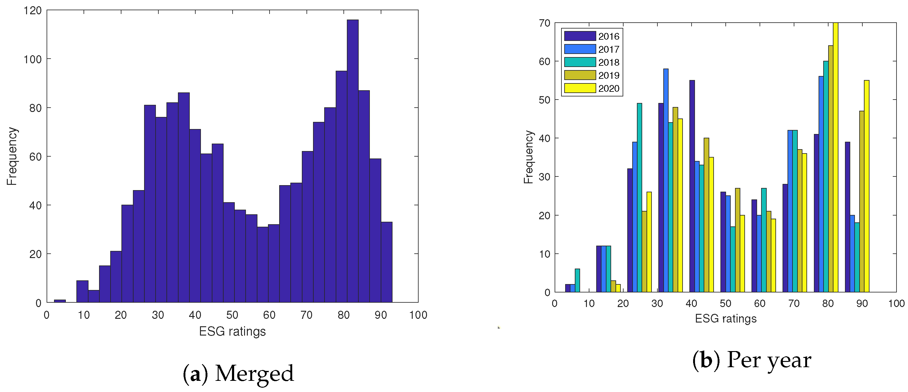
| 3 | 40 points is not arbitrarily chosen. The distribution of the ESG ratings, given in Figure 3a, is bimodal with about 40 points difference between the modes. |
| 4 | We assumed a VAR model of order 1 for simplicity. VAR order could be chosen based on AIC criterion, although typically low orders are preferred. Similarly, Anufriev and Panchenko (2015) and Chiang et al. (2007) use ARMA(1,1) and AR(1) models for simplicity, respectively. Bauwens et al. (2006) note that it is typical that one uses a simple model for conditional mean before applying a multivariate GARCH model. |
| 5 | Given the number of series in consideration including an unobservable factor a la Eratalay and Vladimirov (2020) would not be feasible due to the number of parameters to estimate. |
| 6 | S&P Dow Jones Indices. |
| 7 | https://www.spglobal.com/spdji/en/indices/equity/sp-europe-350/#overview (accesed on 5 October 2020). |
| 8 | On average 0.4% of the returns were identified as outliers. |
| 9 | https://www.spglobal.com/esg/scores/ (accesed on 25 March 2021). |
| 10 | The ESG metrics that different institutions offer weigh these subcategories differently. It is important to obtain ESG ratings data from a reputable source. Berg et al. (2019) point towards the divergence of the ESG metrics provided by different institutions. |
| 11 | https://en.wikipedia.org/wiki/COVID-19_pandemic_in_Europe (accesed on 19 October 2021). |
| 12 | Similar networks were analysed in detail in Cortés Ángel and Eratalay (2021), with the difference that an initial cut-off was used in that study to define a sparse network. In our work, this is not necessary since we are not focusing on finding resilient relationships over time. |
| 13 | Data source: https://sdw.ecb.europa.eu/reports.do?node=1000003285 (accesed on 12 October 2021). |
| 14 | Wirecard AG’s declaration of insolvency did not cause a cascading effect. This is in support of our model that systemic risk contribution and exposure of a firm should be thought of together with the network centrality of that firm. |
| 15 | Given the log-linear relation, we can calculate the exact impact of increase in the regressor x on the dependent variable as . See Chapter 6.2 of Wooldridge (2015) for details. |
References
- Acharya, Viral V., Lasse H. Pedersen, Thomas Philippon, and Matthew Richardson. 2017. Measuring systemic risk. The Review of Financial Studies 30: 2–47. [Google Scholar] [CrossRef]
- Aielli, Gian Piero. 2013. Dynamic conditional correlation: On properties and estimation. Journal of Business & Economic Statistics 31: 282–99. [Google Scholar]
- Anufriev, Mikhail, and Valentyn Panchenko. 2015. Connecting the dots: Econometric methods for uncovering networks with an application to the australian financial institutions. Journal of Banking & Finance 61: S241–S55. [Google Scholar]
- Bae, JinCheol, Xiaotong Yang, and Myung-In Kim. 2021. Esg and stock price crash risk: Role of financial constraints. Asia-Pacific Journal of Financial Studies 50: 556–81. [Google Scholar] [CrossRef]
- Balcilar, Mehmet, Riza Demirer, and Rangan Gupta. 2017. Do sustainable stocks offer diversification benefits for conventional portfolios? an empirical analysis of risk spillovers and dynamic correlations. Sustainability 9: 1799. [Google Scholar] [CrossRef] [Green Version]
- Barigozzi, Matteo, and Christian Brownlees. 2019. Nets: Network estimation for time series. Journal of Applied Econometrics 34: 347–64. [Google Scholar] [CrossRef] [Green Version]
- Bauwens, Luc, Sébastien Laurent, and Jeroen V. K. Rombouts. 2006. Multivariate garch models: A survey. Journal of Applied Econometrics 21: 79–109. [Google Scholar] [CrossRef] [Green Version]
- Benoit, Sylvain, Jean-Edouard Colliard, Christophe Hurlin, and Christophe Pérignon. 2017. Where the risks lie: A survey on systemic risk. Review of Finance 21: 109–52. [Google Scholar] [CrossRef]
- Berg, Florian, Julian F. Koelbel, and Roberto Rigobon. 2019. Aggregate Confusion: The Divergence of ESG Ratings. Boston: MIT Sloan School of Management. [Google Scholar]
- Billio, Monica, Mila Getmansky, Andrew W. Lo, and Loriana Pelizzon. 2012. Econometric measures of connectedness and systemic risk in the finance and insurance sectors. Journal of Financial Economics 104: 535–59. [Google Scholar] [CrossRef]
- Bisias, Dimitrios, Mark Flood, Andrew W. Lo, and Stavros Valavanis. 2012. A survey of systemic risk analytics. Annual Review of Financial Economics 4: 255–96. [Google Scholar] [CrossRef] [Green Version]
- Bollerslev, Tim, and Jeffrey M. Wooldridge. 1992. Quasi-maximum likelihood estimation and inference in dynamic models with time-varying covariances. Econometric Reviews 11: 143–72. [Google Scholar] [CrossRef]
- Boubaker, Sabri, Alexis Cellier, Riadh Manita, and Asif Saeed. 2020. Does corporate social responsibility reduce financial distress risk? Economic Modelling 91: 835–51. [Google Scholar] [CrossRef]
- Bougheas, Spiros, and Alan Kirman. 2015. Complex financial networks and systemic risk: A review. In Complexity and Geographical Economics. Berlin: Springer, pp. 115–39. [Google Scholar]
- Brownlees, Christian, and Robert F. Engle. 2017. Srisk: A conditional capital shortfall measure of systemic risk. The Review of Financial Studies 30: 48–79. [Google Scholar] [CrossRef]
- Caccioli, Fabio, Paolo Barucca, and Teruyoshi Kobayashi. 2018. Network models of financial systemic risk: A review. Journal of Computational Social Science 1: 81–114. [Google Scholar] [CrossRef] [Green Version]
- Capelle-Blancard, Gunther, and Stéphanie Monjon. 2012. Trends in the literature on socially responsible investment: Looking for the keys under the lamppost. Business Ethics: A European Review 21: 239–50. [Google Scholar] [CrossRef] [Green Version]
- Carnero, M. Angeles, and M. Hakan Eratalay. 2014. Estimating var-mgarch models in multiple steps. Studies in Nonlinear Dynamics & Econometrics 18: 339–65. [Google Scholar]
- Cerqueti, Roy, Rocco Ciciretti, Ambrogio Dalò, and Marco Nicolosi. 2021. Esg investing: A chance to reduce systemic risk. Journal of Financial Stability 54: 100887. [Google Scholar] [CrossRef]
- Chiang, Thomas C., Bang Nam Jeon, and Huimin Li. 2007. Dynamic correlation analysis of financial contagion: Evidence from asian markets. Journal of International Money and Finance 26: 1206–28. [Google Scholar] [CrossRef]
- Chiaramonte, Laura, Alberto Dreassi, Claudia Girardone, and Stefano Piserà. 2021. Do esg strategies enhance bank stability during financial turmoil? Evidence from europe. In The European Journal of Finance. Abingdon: Taylor & Francis, pp. 1–39. [Google Scholar]
- Clark, Gordon L., Andreas Feiner, and Michael Viehs. 2015. From the Stockholder to the Stakeholder: How Sustainability Can Drive Financial Outperformance. Available online: https://papers.ssrn.com/sol3/papers.cfm?abstract_id=2508281 (accessed on 2 January 2022).
- Cortés Ángel, Ariana Paola, and Mustafa Hakan Eratalay. 2021. Deep Diving into the s&p Europe 350 Index Network and Its Reaction to COVID-19. Available online: https://papers.ssrn.com/sol3/papers.cfm?abstract_id=3964652 (accessed on 14 December 2021).
- Cortez, Maria Ceu, Florinda Silva, and Nelson Areal. 2009. The performance of european socially responsible funds. Journal of Business Ethics 87: 573–88. [Google Scholar] [CrossRef]
- Cortez, Maria Céu, Florinda Silva, and Nelson Areal. 2012. Socially responsible investing in the global market: The performance of us and european funds. International Journal of Finance & Economics 17: 254–71. [Google Scholar]
- De Bandt, Olivier, and Philipp Hartmann. 2000. Systemic Risk: A Survey. Available online: https://papers.ssrn.com/sol3/papers.cfm?abstract_id=258430 (accessed on 5 January 2022).
- Dorfleitner, Gregor, Gerhard Halbritter, and Mai Nguyen. 2015. Measuring the level and risk of corporate responsibility—An empirical comparison of different esg rating approaches. Journal of Asset Management 16: 450–66. [Google Scholar] [CrossRef]
- Drempetic, Samuel, Christian Klein, and Bernhard Zwergel. 2020. The influence of firm size on the esg score: Corporate sustainability ratings under review. Journal of Business Ethics 167: 333–60. [Google Scholar] [CrossRef]
- Engle, Robert. 2002. Dynamic conditional correlation: A simple class of multivariate generalized autoregressive conditional heteroskedasticity models. Journal of Business & Economic Statistics 20: 339–50. [Google Scholar]
- Eratalay, M. Hakan. 2021. Financial econometrics and systemic risk. In Handbook of Research on Emerging Theories, Models, and Applications of Financial Econometrics. Berlin: Springer, pp. 65–91. [Google Scholar]
- Eratalay, M. Hakan, and Evgenii V. Vladimirov. 2020. Mapping the stocks in micex: Who is central in the moscow stock exchange? Economics of Transition and Institutional Change 28: 581–620. [Google Scholar] [CrossRef]
- Escrig-Olmedo, Elena, María Ángeles Fernández-Izquierdo, Idoya Ferrero-Ferrero, Juana María Rivera-Lirio, and María Jesús Muñoz-Torres. 2019. Rating the raters: Evaluating how esg rating agencies integrate sustainability principles. Sustainability 11: 915. [Google Scholar] [CrossRef] [Green Version]
- Friede, Gunnar, Timo Busch, and Alexander Bassen. 2015. Esg and financial performance: Aggregated evidence from more than 2000 empirical studies. Journal of Sustainable Finance & Investment 5: 210–33. [Google Scholar]
- Ghysels, Eric, Andrew C. Harvey, and Eric Renault. 1996. 5 stochastic volatility. Handbook of Statistics 14: 119–91. [Google Scholar]
- Giese, Guido, Linda-Eling Lee, Dimitris Melas, Zoltán Nagy, and Laura Nishikawa. 2019. Foundations of esg investing: How esg affects equity valuation, risk, and performance. The Journal of Portfolio Management 45: 69–83. [Google Scholar] [CrossRef]
- Gray, Dale F., Robert C. Merton, and Zvi Bodie. 2007. New Framework for Measuring and Managing Macrofinancial Risk and Financial Stability. Technical Report. Cambridge: National Bureau of Economic Research. [Google Scholar]
- Green, Samuel B. 1991. How many subjects does it take to do a regression analysis. Multivariate Behavioral Research 26: 499–510. [Google Scholar] [CrossRef]
- Gregory, Richard Paul. 2022. Esg scores and the response of the s&p 1500 to monetary and fiscal policy during the COVID-19 pandemic. International Review of Economics & Finance 78: 446–56. [Google Scholar]
- Harrell, Frank E. 2001. Regression Modeling Strategies: With Applications to Linear Models, Logistic Regression, and Survival Analysis. Berlin: Springer, vol. 608. [Google Scholar]
- Hollo, Daniel, Manfred Kremer, and Marco Lo Duca. 2012. Ciss—A Composite Indicator of Systemic Stress in the Financial System. Frankfurt: European Central Bank. [Google Scholar]
- Hox, Joop J., Mirjam Moerbeek, and Rens Van de Schoot. 2017. Multilevel Analysis: Techniques and Applications. Hoboken: Routledge. [Google Scholar]
- Ionescu, George H., Daniela Firoiu, Ramona Pirvu, and Ruxandra Dana Vilag. 2019. The impact of esg factors on market value of companies from travel and tourism industry. Technological and Economic Development of Economy 25: 820–49. [Google Scholar] [CrossRef]
- Jackson, Matthew O. 2010. Social and Economic Networks. Princeton: Princeton University Press. [Google Scholar]
- Jain, Mansi, Gagan Deep Sharma, and Mrinalini Srivastava. 2019. Can sustainable investment yield better financial returns: A comparative study of esg indices and msci indices. Risks 7: 15. [Google Scholar] [CrossRef] [Green Version]
- Jin, Ick. 2018. Is esg a systematic risk factor for us equity mutual funds? Journal of Sustainable Finance & Investment 8: 72–93. [Google Scholar]
- Klooster, Sophie van’t. 2018. The Impact of CSR on Default and Systemic Risk in the European Banking Sector. Ph. D. thesis, Faculty of Economics and Business, University of Groningen, Groningen, The Netherlands. [Google Scholar]
- Kritzman, Mark, Yuanzhen Li, Sebastien Page, and Roberto Rigobon. 2011. Principal components as a measure of systemic risk. The Journal of Portfolio Management 37: 112–26. [Google Scholar] [CrossRef] [Green Version]
- Lai, Chi-Shiun, Chih-Jen Chiu, Chin-Fang Yang, and Da-Chang Pai. 2010. The effects of corporate social responsibility on brand performance: The mediating effect of industrial brand equity and corporate reputation. Journal of Business Ethics 95: 457–69. [Google Scholar] [CrossRef]
- Lee, Darren D., Robert W. Faff, and Saphira A. C. Rekker. 2013. Do high and low-ranked sustainability stocks perform differently? International Journal of Accounting & Information Management 21: 116–32. [Google Scholar]
- Lehar, Alfred. 2005. Measuring systemic risk: A risk management approach. Journal of Banking & Finance 29: 2577–603. [Google Scholar]
- Leterme, Johan, and Anh Nguyen. 2020. Can Esg Factors Be Considered as a Systematic Risk Factor for Equity Mutual Funds in the Eurozone? Available online: http://hdl.handle.net/2078.1/thesis:24176 (accessed on 10 January 2022).
- Liu, Jianxu, Quanrui Song, Yang Qi, Sanzidur Rahman, and Songsak Sriboonchitta. 2020. Measurement of systemic risk in global financial markets and its application in forecasting trading decisions. Sustainability 12: 4000. [Google Scholar] [CrossRef]
- Lööf, Hans, Maziar Sahamkhadam, and Andreas Stephan. 2021. Is corporate social responsibility investing a free lunch? the relationship between esg, tail risk, and upside potential of stocks before and during the covid-19 crisis. Finance Research Letters 2021: 102499. [Google Scholar] [CrossRef]
- Lopez-de Silanes, Florencio, Joseph A. McCahery, and Paul C. Pudschedl. 2020. Esg performance and disclosure: A cross-country analysis. Singapore Journal of Legal Studies 2020: 217–41. [Google Scholar]
- Lundgren, Amanda Ivarsson, Adriana Milicevic, Gazi Salah Uddin, and Sang Hoon Kang. 2018. Connectedness network and dependence structure mechanism in green investments. Energy Economics 72: 145–53. [Google Scholar] [CrossRef]
- Maiti, Moinak. 2021. Is esg the succeeding risk factor? Journal of Sustainable Finance & Investment 11: 199–213. [Google Scholar]
- Michelon, Giovanna. 2011. Sustainability disclosure and reputation: A comparative study. Corporate Reputation Review 14: 79–96. [Google Scholar] [CrossRef]
- Murè, Pina, Marco Spallone, Fabiomassimo Mango, Stefano Marzioni, and Lucilla Bittucci. 2021. Esg and reputation: The case of sanctioned italian banks. Corporate Social Responsibility and Environmental Management 28: 265–77. [Google Scholar] [CrossRef]
- Oikonomou, Ioannis, Chris Brooks, and Stephen Pavelin. 2012. The impact of corporate social performance on financial risk and utility: A longitudinal analysis. Financial Management 41: 483–515. [Google Scholar] [CrossRef] [Green Version]
- Pakel, Cavit, Neil Shephard, Kevin Sheppard, and Robert F. Engle. 2020. Fitting vast dimensional time-varying covariance models. Journal of Business & Economic Statistics 39: 652–68. [Google Scholar]
- Pearson, Ronald K., Yrjö Neuvo, Jaakko Astola, and Moncef Gabbouj. 2015. The class of generalized hampel filters. Paper presented at the 2015 23rd European Signal Processing Conference (EUSIPCO), Nice, France, August 31–September 4; pp. 2501–5. [Google Scholar]
- Reboredo, Juan C., Andrea Ugolini, and Fernando Antonio Lucena Aiube. 2020. Network connectedness of green bonds and asset classes. Energy Economics 86: 104629. [Google Scholar] [CrossRef]
- Revelli, Christophe, and Jean-Laurent Viviani. 2015. Financial performance of socially responsible investing (sri): What have we learned? a meta-analysis. Business Ethics: A European Review 24: 158–85. [Google Scholar] [CrossRef]
- Silva, Thiago Christiano, Michel Alexandre da Silva, and Benjamin Miranda Tabak. 2017. Systemic risk in financial systems: A feedback approach. Journal of Economic Behavior & Organization 144: 97–120. [Google Scholar]
- Sonnenberger, David, and Gregor N. F. Weiss. 2021. The Impact of Corporate Social Responsibility on Firms’ Exposure to Tail Risk: The Case of Insurers. Available online: https://papers.ssrn.com/sol3/papers.cfm?abstract_id=3764041 (accessed on 5 January 2022).
- Sun, Wenbin, and Kexiu Cui. 2014. Linking corporate social responsibility to firm default risk. European Management Journal 32: 275–87. [Google Scholar] [CrossRef]
- Tarashev, Nikola A., Claudio E. V. Borio, and Kostas Tsatsaronis. 2010. Attributing Systemic Risk to Individual Institutions. Available online: https://papers.ssrn.com/sol3/papers.cfm?abstract_id=1631761 (accessed on 4 January 2022).
- Tobias, Adrian, and Markus K. Brunnermeier. 2016. Covar. The American Economic Review 106: 1705. [Google Scholar]
- Waner, Zhao. 2021. Research on the relationship between social responsibility and systemic risk. AGE 7: 2321–32. [Google Scholar]
- Wooldridge, Jeffrey M. 2015. Introductory Econometrics: A Modern Approach. Boston: Cengage Learning. [Google Scholar]
- Zhao, Shangmei, Xinyi Chen, and Junhuan Zhang. 2019. The systemic risk of china’s stock market during the crashes in 2008 and 2015. Physica A: Statistical Mechanics and its Applications 520: 161–77. [Google Scholar] [CrossRef]

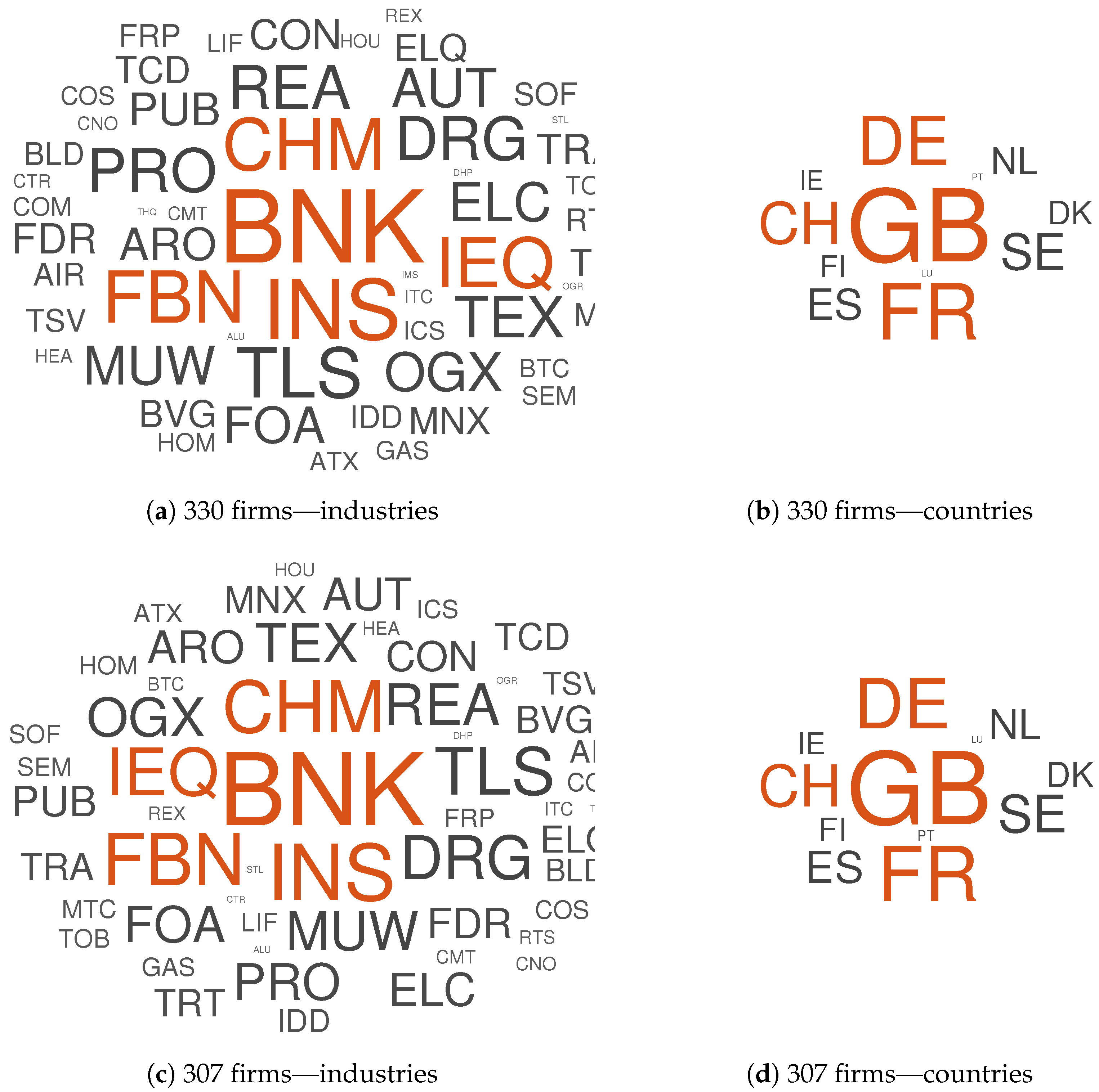
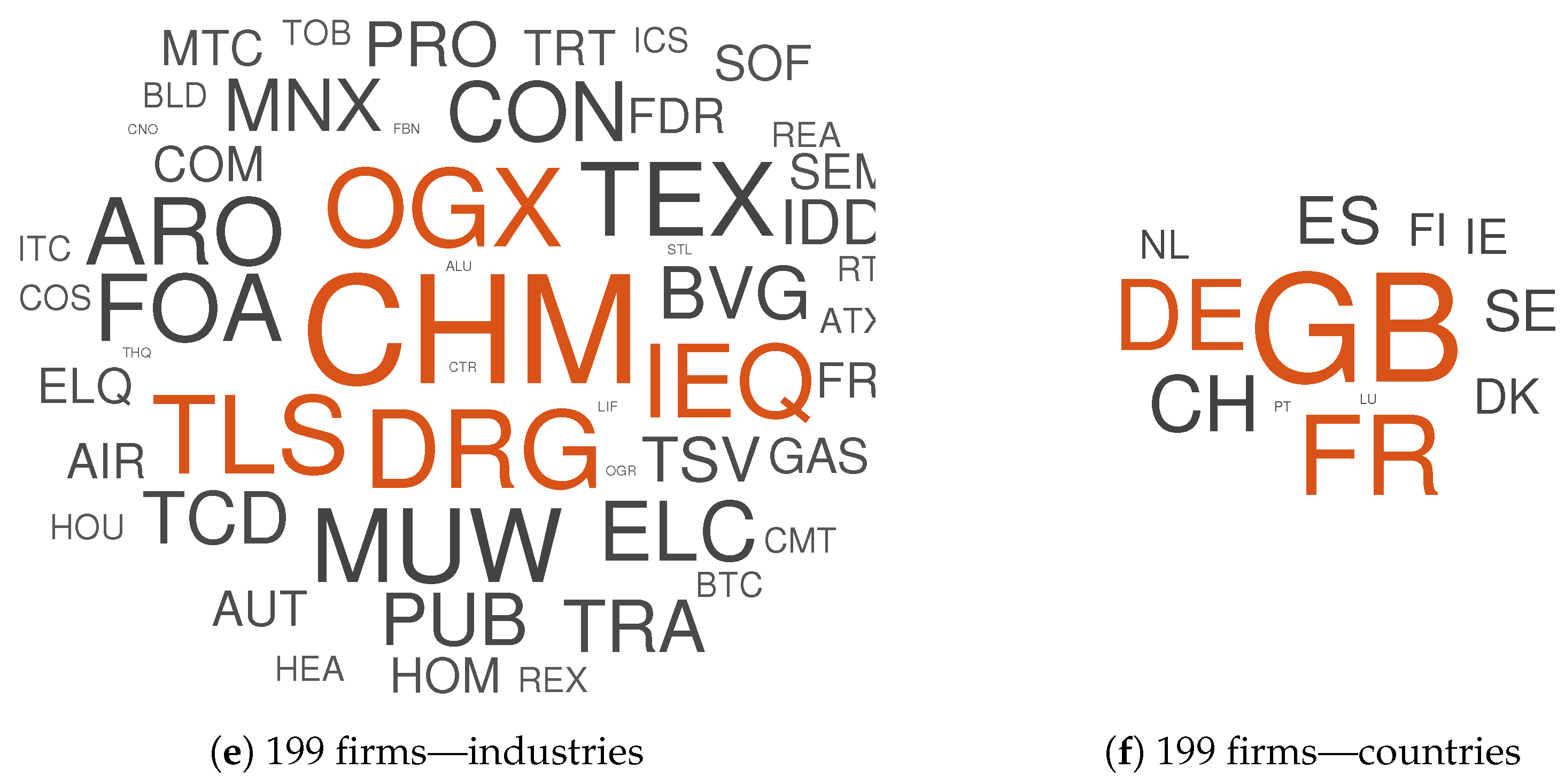
| Panels | Description | Number of Stocks |
|---|---|---|
| Panel 1 | The stocks for which systemic risk, volatility and network centralities were calculated. | 331 |
| Panel 2 | The stocks of Panel 1, for which we could obtain ESG ratings data. | 308 |
| Panel 3 | The stocks of Panel 2, for which we could obtain financial performance ratios. | 200 |
| Countries | 2016 | 2017 | 2018 | 2019 | 2020 | Count |
|---|---|---|---|---|---|---|
| Germany | 57.79 | 56.24 | 48.68 | 50.11 | 49.97 | 38 |
| France | 70.82 | 69.24 | 61.11 | 60.42 | 59.93 | 45 |
| Luxembourg | 40.50 | 49.00 | 38.50 | 40.00 | 39.50 | 2 |
| Ireland | 46.22 | 46.56 | 37.22 | 37.44 | 38.11 | 9 |
| Italy | 70.38 | 69.31 | 67.69 | 70.62 | 72.31 | 13 |
| Belgium | 44.00 | 44.63 | 35.50 | 39.75 | 43.75 | 8 |
| Denmark | 53.10 | 50.40 | 41.00 | 37.80 | 35.90 | 10 |
| Norway | 53.57 | 50.00 | 43.43 | 43.71 | 43.43 | 7 |
| Spain | 75.12 | 73.94 | 67.41 | 68.65 | 71.41 | 17 |
| Sweden | 54.55 | 51.50 | 41.95 | 44.14 | 46.86 | 22 |
| Netherlands | 71.82 | 72.53 | 65.06 | 62.24 | 60.59 | 17 |
| Portugal | 84.00 | 84.00 | 80.50 | 86.00 | 85.00 | 2 |
| Austria | 55.00 | 59.00 | 58.00 | 61.00 | 61.50 | 2 |
| Finland | 62.78 | 58.56 | 52.33 | 50.22 | 51.78 | 9 |
| Switzerland | 59.00 | 57.86 | 52.45 | 52.79 | 54.59 | 29 |
| United Kingdom | 58.76 | 56.54 | 49.27 | 50.23 | 51.10 | 78 |
| Short Name | Variable |
|---|---|
| NetEC | Net eigenvector centrality |
| AbsCC | Absolute value closeness centrality |
| logVol | Natural logarithm of volatility |
| Dt | Dummy variable, equals 1 for year 2020 |
| ESGrating | ESG rating of the company |
| CR | Current ratio |
| PM | Profit margin |
| SR | Solvency ratio |
| Sample → | All | Southern | Northern | ||||||
|---|---|---|---|---|---|---|---|---|---|
| Coef. | St. Err. | Sig. | Coef. | St. Err. | Sig. | Coef. | St. Err. | Sig. | |
| NetEC | 8.3727 | 2.1479 | *** | 7.7652 | 4.3691 | * | 8.5689 | 2.5133 | *** |
| AbsCC | 64.4704 | 7.4758 | *** | 67.3261 | 15.7056 | *** | 63.3571 | 8.5363 | *** |
| logVol | 1.6429 | 0.0566 | *** | 1.6423 | 0.1127 | *** | 1.6603 | 0.0677 | *** |
| NetEC*logVol | −0.3447 | 0.8094 | 0.0288 | 1.4331 | −0.8337 | 1.0174 | |||
| Dt | −0.4329 | 0.0156 | *** | −0.4449 | 0.0326 | *** | −0.4335 | 0.0189 | *** |
| NetEC*Dt | 1.6016 | 0.3159 | *** | 1.5794 | 0.6146 | ** | 1.7127 | 0.3897 | *** |
| logVol*Dt | 0.0833 | 0.0134 | *** | 0.0897 | 0.0297 | *** | 0.0811 | 0.0152 | *** |
| _cons | −3.7423 | 0.4821 | *** | −3.9077 | 1.0674 | *** | −3.6757 | 0.5399 | *** |
| Corr(u,X) | 0.2968 | 0.1615 | 0.3548 | ||||||
| Pval_Ftest | 0.0000 | 0.0000 | 0.0000 | ||||||
| within | 0.8862 | 0.8984 | 0.8809 | ||||||
| between | 0.8941 | 0.8834 | 0.8998 | ||||||
| overall | 0.8923 | 0.8847 | 0.8967 | ||||||
| sigma_u | 0.3159 | 0.2974 | 0.3220 | ||||||
| sigma_e | 0.1082 | 0.1099 | 0.1080 | ||||||
| rho | 0.8949 | 0.8799 | 0.8989 | ||||||
| N | 330 | 90 | 240 |
| Sample → | All | Southern | Northern | ||||||
|---|---|---|---|---|---|---|---|---|---|
| Coef. | St. Err. | Sig. | Coef. | St. Err. | Sig. | Coef. | St. Err. | Sig. | |
| NetEC | 8.7535 | 2.2502 | *** | 9.6099 | 4.7321 | ** | 8.4713 | 2.6003 | *** |
| AbsCC | 68.5705 | 7.7649 | *** | 67.5842 | 17.1712 | *** | 68.8595 | 8.6944 | *** |
| ESGrating | −0.0007 | 0.0004 | * | −0.0005 | 0.0008 | −0.0009 | 0.0005 | * | |
| logVol | 1.6316 | 0.0568 | *** | 1.6710 | 0.1203 | *** | 1.6373 | 0.0677 | *** |
| NetEC*logVol | −0.1281 | 0.7984 | −0.3629 | 1.5245 | −0.4371 | 0.9981 | |||
| Dt | −0.4264 | 0.0204 | *** | −0.4501 | 0.0535 | *** | −0.4252 | 0.0242 | *** |
| NetEC*Dt | 1.5115 | 0.3464 | *** | 1.7231 | 0.8141 | ** | 1.5537 | 0.3977 | *** |
| logVol*Dt | 0.0856 | 0.0145 | *** | 0.0908 | 0.0329 | *** | 0.0848 | 0.0164 | *** |
| ESGrating*Dt | 0.0000 | 0.0002 | −0.0000 | 0.0006 | 0.0000 | 0.0003 | |||
| _cons | −3.9823 | 0.5009 | *** | −4.0233 | 1.1596 | *** | −3.9669 | 0.5528 | *** |
| Corr(u,X) | 0.2382 | 0.0669 | 0.3105 | ||||||
| Pval_Ftest | 0.0000 | 0.0000 | 0.0000 | ||||||
| within | 0.8896 | 0.9042 | 0.8832 | ||||||
| between | 0.8895 | 0.8729 | 0.8976 | ||||||
| overall | 0.8888 | 0.8766 | 0.8953 | ||||||
| sigma_u | 0.3159 | 0.3068 | 0.3179 | ||||||
| sigma_e | 0.1079 | 0.1102 | 0.1075 | ||||||
| rho | 0.8955 | 0.8858 | 0.8973 | ||||||
| N | 307 | 81 | 226 |
| Sample → | All | Southern | Northern | ||||||
|---|---|---|---|---|---|---|---|---|---|
| Coef. | St. Err. | Sig. | Coef. | St. Err. | Sig. | Coef. | St. Err. | Sig. | |
| NetEC | 9.8011 | 4.2693 | ** | 14.0324 | 8.0976 | * | 8.4767 | 4.8918 | * |
| AbsCC | 78.7130 | 9.2521 | *** | 81.1382 | 24.4414 | *** | 79.4319 | 10.2511 | *** |
| ESGrating | −0.0012 | 0.0005 | ** | −0.0019 | 0.0010 | * | −0.0010 | 0.0006 | * |
| CR | 0.0639 | 0.0298 | ** | 0.0938 | 0.1230 | 0.0710 | 0.0310 | ** | |
| PM | 0.0048 | 0.0013 | *** | 0.0012 | 0.0037 | 0.0044 | 0.0014 | *** | |
| SR | 0.0005 | 0.0035 | −0.0012 | 0.0070 | 0.0003 | 0.0038 | |||
| logVol | 1.7410 | 0.0815 | *** | 1.4485 | 0.2155 | *** | 1.7312 | 0.0887 | *** |
| NetEC*logVol | −0.4065 | 1.4020 | 3.0364 | 3.0377 | −0.0675 | 1.6459 | |||
| NetEC*CR | −0.8164 | 0.6741 | −1.5913 | 2.3496 | −1.1342 | 0.7412 | |||
| NetEC*PM | −0.0702 | 0.0208 | *** | 0.0059 | 0.0702 | −0.0603 | 0.0276 | ** | |
| NetEC*SR | 0.0405 | 0.0774 | 0.0768 | 0.1223 | 0.0487 | 0.0874 | |||
| logVol*CR | −0.0198 | 0.0206 | 0.1562 | 0.1043 | −0.0245 | 0.0215 | |||
| logVol*PM | −0.0017 | 0.0006 | *** | −0.0027 | 0.0018 | −0.0017 | 0.0006 | *** | |
| logVol*SR | −0.0028 | 0.0010 | *** | −0.0081 | 0.0030 | *** | −0.0023 | 0.0011 | ** |
| Dt | −0.3793 | 0.0320 | *** | −0.3194 | 0.1227 | ** | −0.3573 | 0.0351 | *** |
| NetEC*Dt | 2.0518 | 0.4654 | *** | 1.7539 | 1.1584 | 1.7616 | 0.5330 | *** | |
| logVol*Dt | 0.0424 | 0.0196 | ** | 0.0510 | 0.0398 | 0.0442 | 0.0217 | ** | |
| ESGrating*Dt | −0.0002 | 0.0003 | −0.0007 | 0.0009 | −0.0002 | 0.0003 | |||
| CR*Dt | −0.0067 | 0.0050 | −0.0837 | 0.0465 | * | −0.0033 | 0.0044 | ||
| PM*Dt | −0.0004 | 0.0007 | −0.0005 | 0.0011 | −0.0003 | 0.0008 | |||
| SR*Dt | −0.0003 | 0.0004 | 0.0027 | 0.0009 | *** | −0.0008 | 0.0004 | * | |
| _cons | −4.7024 | 0.5948 | *** | −5.0623 | 1.6964 | *** | −4.6851 | 0.6372 | *** |
| Corr(u,X) | 0.3076 | 0.0330 | 0.3514 | ||||||
| Pval_Ftest | 0.0000 | 0.0000 | 0.0000 | ||||||
| within | 0.8673 | 0.8837 | 0.8646 | ||||||
| between | 0.8770 | 0.6809 | 0.9025 | ||||||
| overall | 0.8750 | 0.7033 | 0.8987 | ||||||
| sigma_u | 0.3417 | 0.4237 | 0.3277 | ||||||
| sigma_e | 0.1083 | 0.1053 | 0.1099 | ||||||
| rho | 0.9087 | 0.9415 | 0.8988 | ||||||
| N | 199 | 52 | 147 |
| Sample → | All | Southern | Northern | ||||||
|---|---|---|---|---|---|---|---|---|---|
| Coef. | St. Err. | Sig. | Coef. | St. Err. | Sig. | Coef. | St. Err. | Sig. | |
| NetEC | −1.4137 | 0.3312 | *** | −1.5600 | 0.5433 | *** | −1.2293 | 0.3705 | *** |
| AbsCC | 1.9125 | 0.9787 | * | 3.1472 | 1.6868 | * | 1.3937 | 1.2022 | |
| logVol | 2.0993 | 0.0185 | *** | 2.0978 | 0.0305 | *** | 2.1112 | 0.0214 | *** |
| NetEC*logVol | 0.0004 | 0.3492 | 0.2293 | 0.5132 | −0.3245 | 0.4147 | |||
| _cons | −0.1098 | 0.0616 | * | −0.1844 | 0.1003 | * | −0.0844 | 0.0757 | |
| Pval_Ftest | 0.0000 | 0.0000 | 0.0000 | ||||||
| 0.9984 | 0.9983 | 0.9984 | |||||||
| N | 330 | 90 | 240 |
| Sample → | All | Southern | Northern | ||||||
|---|---|---|---|---|---|---|---|---|---|
| Coef. | St. Err. | Sig. | Coef. | St. Err. | Sig. | Coef. | St. Err. | Sig. | |
| NetEC | −1.5043 | 0.3474 | *** | −1.3615 | 0.6195 | ** | −1.3497 | 0.4002 | *** |
| AbsCC | 2.2423 | 1.0341 | * | 2.4784 | 1.8449 | 1.9141 | 1.2944 | ||
| Esg_Env | −0.0003 | 0.0002 | 0.0001 | 0.0003 | −0.0003 | 0.0002 | |||
| Esg_Soc | 0.0001 | 0.0002 | 0.0005 | 0.0009 | 0.0000 | 0.0003 | |||
| Esg_GovEcon | 0.0002 | 0.0003 | −0.0003 | 0.0008 | 0.0003 | 0.0003 | |||
| logVol | 2.0881 | 0.0199 | *** | 2.0961 | 0.0316 | *** | 2.0980 | 0.0240 | *** |
| NetEC*logVol | 0.1710 | 0.3727 | 0.2201 | 0.5437 | −0.1165 | 0.4639 | |||
| _cons | −0.1233 | 0.0645 | * | −0.1743 | 0.1054 | −0.1040 | 0.0803 | ||
| Pval_Ftest | 0.0000 | 0.0000 | 0.0000 | ||||||
| 0.9984 | 0.9984 | 0.9985 | |||||||
| N | 307 | 81 | 226 |
| Sample → | All | Southern | Northern | ||||||
|---|---|---|---|---|---|---|---|---|---|
| Coef. | St. Err. | Sig. | Coef. | St. Err. | Sig. | Coef. | St. Err. | Sig. | |
| NetEC | −1.4657 | 0.6431 | ** | −1.8380 | 1.1139 | −1.2013 | 0.7311 | ||
| AbsCC | 0.2549 | 1.1934 | 0.6408 | 2.8673 | −0.2989 | 1.4799 | |||
| Esg_Env | −0.0001 | 0.0003 | −0.0013 | 0.0012 | 0.0001 | 0.0003 | |||
| Esg_Soc | 0.0008 | 0.0004 | ** | 0.0013 | 0.0013 | 0.0007 | 0.0003 | ** | |
| Esg_GovEcon | −0.0009 | 0.0003 | *** | −0.0007 | 0.0006 | −0.0008 | 0.0003 | ** | |
| CR | −0.0134 | 0.0087 | −0.1310 | 0.0444 | *** | −0.0059 | 0.0079 | ||
| PM | 0.0006 | 0.0006 | 0.0014 | 0.0010 | 0.0003 | 0.0007 | |||
| SR | 0.0001 | 0.0007 | 0.0035 | 0.0021 | 0.0002 | 0.0008 | |||
| logVol | 2.1108 | 0.0234 | *** | 2.1396 | 0.0570 | *** | 2.1115 | 0.0261 | *** |
| NetEC*logVol | −0.2389 | 0.4411 | −0.8308 | 1.0937 | −0.3030 | 0.5026 | |||
| NetEC*CR | 0.2170 | 0.1769 | 2.0354 | 0.7527 | *** | 0.1001 | 0.1482 | ||
| NetEC*PM | −0.0113 | 0.0109 | −0.0314 | 0.0193 | −0.0041 | 0.0133 | |||
| NetEC*SR | −0.0001 | 0.0115 | −0.0534 | 0.0366 | −0.0039 | 0.0131 | |||
| _cons | 0.0079 | 0.0766 | 0.0608 | 0.1744 | 0.0151 | 0.0926 | |||
| Pval_Ftest | 0.0000 | 0.0000 | 0.0000 | ||||||
| 0.9985 | 0.9983 | 0.9988 | |||||||
| N | 199 | 52 | 147 |
| Panel: 307 Stocks | ESG Coef | St. Err. | Pval | D*ESG Coef | St. Err. | Pval | N |
|---|---|---|---|---|---|---|---|
| Communication Services | −0.0025 | 0.0015 | −0.0014 | 0.0011 | 19 | ||
| Consumer Discretionary | 0.0006 | 0.0010 | 0.0014 | 0.0006 | ** | 32 | |
| Consumer Staples | 0.0007 | 0.0013 | −0.0006 | 0.0005 | 29 | ||
| Energy | −0.0045 | 0.0020 | * | 0.0048 | 0.0028 | 10 | |
| Financials | −0.0016 | 0.0007 | ** | −0.0004 | 0.0005 | 59 | |
| Health Care | −0.0011 | 0.0023 | 0.0001 | 0.0010 | 21 | ||
| Industrials | −0.0007 | 0.0009 | 0.0005 | 0.0006 | 64 | ||
| Information Technology | −0.0026 | 0.0016 | 0.0022 | 0.0010 | * | 15 | |
| Materials | −0.0005 | 0.0008 | −0.0006 | 0.0008 | 29 | ||
| Real Estate | 0.0004 | 0.0026 | −0.0042 | 0.0021 | * | 10 | |
| Utilities | −0.0048 | 0.0012 | *** | −0.0010 | 0.0012 | 19 | |
| Panel: 199 Stocks | ESG Coef | St. Err. | Sig. | D*ESG Coef | St. Err. | Sig | N |
| Communication Services | −0.0015 | 0.0028 | −0.0033 | 0.0013 | ** | 14 | |
| Consumer Discretionary | 0.0009 | 0.0018 | −0.0008 | 0.0008 | 22 | ||
| Consumer Staples | 0.0013 | 0.0016 | −0.0003 | 0.0009 | 23 | ||
| Energy | −0.0061 | 0.0035 | 0.0102 | 0.0021 | *** | 10 | |
| Financials | - | - | - | - | - | - | 1 |
| Health Care | −0.0064 | 0.0020 | *** | 0.0025 | 0.0011 | ** | 17 |
| Industrials | −0.0003 | 0.0015 | −0.0005 | 0.0009 | 49 | ||
| Information Technology | −0.0035 | 0.0011 | *** | 0.0026 | 0.0016 | 15 | |
| Materials | −0.0009 | 0.0008 | −0.0004 | 0.0007 | 29 | ||
| Real Estate | - | - | - | - | - | - | 2 |
| Utilities | −0.0052 | 0.0019 | ** | −0.0007 | 0.0020 | 17 |
Publisher’s Note: MDPI stays neutral with regard to jurisdictional claims in published maps and institutional affiliations. |
© 2022 by the authors. Licensee MDPI, Basel, Switzerland. This article is an open access article distributed under the terms and conditions of the Creative Commons Attribution (CC BY) license (https://creativecommons.org/licenses/by/4.0/).
Share and Cite
Eratalay, M.H.; Cortés Ángel, A.P. The Impact of ESG Ratings on the Systemic Risk of European Blue-Chip Firms. J. Risk Financial Manag. 2022, 15, 153. https://doi.org/10.3390/jrfm15040153
Eratalay MH, Cortés Ángel AP. The Impact of ESG Ratings on the Systemic Risk of European Blue-Chip Firms. Journal of Risk and Financial Management. 2022; 15(4):153. https://doi.org/10.3390/jrfm15040153
Chicago/Turabian StyleEratalay, Mustafa Hakan, and Ariana Paola Cortés Ángel. 2022. "The Impact of ESG Ratings on the Systemic Risk of European Blue-Chip Firms" Journal of Risk and Financial Management 15, no. 4: 153. https://doi.org/10.3390/jrfm15040153