Does Volume of Gold Consumption Influence the World Gold Price?

Abstract

Gold is a universal commodity traded across the world. The London Bullion Market Association (LBMA) fixes prices twice a day, known as AM and PM fix prices. This study is an attempt to find out whether the volume of gold consumption shows any significant impact on the world gold prices, known as LBMA fix prices. The sample includes major gold-consuming countries, such as India, the USA, China, Japan, and countries in Europe and the Middle East grouped together under Europe and the Middle East, respectively. The results conclude that there exists a long-run relationship between LBMA fix prices and the gold demand of all the countries. Furthermore, the volume of gold demand significantly influences LBMA AM fix and PM fix prices. It is found out that the demand of all the countries together, and India and China individually, affect the world gold prices significantly. India consistently stands as the largest consumer of gold in the world gold market. In spite of this, India is a price taker. Bullion associations and commodity exchanges that allow bullion trade in India may take initiatives to make India a price maker in the world gold markets.

1. Introduction

Gold is a universal and virtually indestructible commodity that has a unique emotional, cultural, and financial value. The annual gold demand has seen threefold growth since 1970 and gold markets have widened massively across the world. From the supply side, 75% of gold demand is met through mine production and the rest comes from the recycling of jewellery. As per the World Gold Council estimation, around 205,238 tonnes of gold have been mined throughout history. Some of the major gold markets in the world are London, the USA, China, Dubai, India, Japan, Singapore, Turkey, and Hong Kong.

Different people across the globe buy gold for different purposes (Starr and Tran 2008). In China, there is a tradition that tiny necklaces and bracelets are gifted to new-born babies. For centuries, the use of wedding rings is part of Western European culture. The major driver of demand for gold jewellery in the USA is weddings (Shafiee and Topal 2010). In India, the demand for gold is found not only during special occasions, such as festivals, weddings, etc., but throughout the year. Around seventy percent of its consumption remains unaffected irrespective of the fluctuations in the price and economic conditions. The Indian calendar even has auspicious days to buy gold, such as Dhanteras and Dassera. History shows that gold has always been a central part of the socioeconomic ethos of Indian households (Bhattacharya 2002). After China, India is the second-largest importer of gold in the world gold markets. Indians seldom recycle gold jewellery and keep buying fresh gold every time in the form of jewellery. This creates a deficit in the current account and has become more of a burden for the Indian economy (Dan Popescu 2014).

The price associated with the spot market is also known as the benchmark price fixed by the London Bullion Market Association (LBMA) AM Fix and PM fix prices. The spot gold price is actually fixed at the LBMA by its members twice a day, but what makes them fix the benchmark price? Economic theory states that the price of a commodity is determined by both supply and demand. Gold is one of the precious metal commodities traded across the world and its demand and supply will have an impact on its price. Earlier studies, such as by Selvanathan and Selvanathan (1999), suggested that both ‘gold price and production are not cointegrated and there is no long-run relationship between the gold price and production. Production did not show any impact on the price. Hence, this study focuses on the demand aspect. This study addresses the following research questions: Is there a long-run relationship between gold demand and its price? Whose demand plays a significant role in price fixation? Do the international gold prices show any reaction to the changes in gold demand? Our findings may contribute to the literature on the impact of physical gold demand on the international benchmark price. We hardly find any research in this area.

This paper is structured as follows: Section 2 discusses the existing literature relevant to the study, Section 3 provides information on objectives, variables, and methodologies used in the analysis, Section 4 and Section 5 describe the results and conclusion, respectively.

2. Review of Literature

O’Connor et al. (2015) made a comprehensive study of the literature on world gold markets. The study reviewed and documented around two hundred research articles published on different dimensions of world gold markets. Many research articles have argued that spot gold price is derived from the paper market and not from the physical market, as the volume of transactions is very high. They have not only explained the price-setting mechanism but also described the drawbacks Aasif (2018), BullionStar (2017a). Hauptfleisch et al. (2016) used intraday data from the London spot market and New York futures market to find out who set the gold price. They concluded that the New York futures play a larger role than the London spot market. The price discovery is also influenced by the daylight hours, as the London spot market plays a more important role during UK daylight hours and the US futures market plays a more important role during US daylight hours. However, the limitation of the study is that it ignored the other major gold-consuming countries in the analysis.

Lucey et al. (2013) analysed the information share in the price fixation between London and New York. The study concluded that neither market dominated the price fixation permanently. Lucey et al. (2014) extended their previous study by including two more markets, Tokyo and Shanghai, and examined the return and volatility spillover effect. The London cash market and COMEX dominated the spillover more than the other two markets. Lin et al. (2018) analysed the cross-correlations among five major gold markets: London, New York, Shanghai, Tokyo, and Mumbai. The study concluded that the cross-correlations, net cross-correlations, and net influences among the five gold markets vary across time scales. The London gold market significantly affects the other four gold markets and dominates the worldwide gold market. This study considered only the futures prices and the spot prices. The impact of physical demand is also not included in the analysis.

Yurdakul and Sefa (2015) analysed the factors that affect gold prices on the Turkish Gold Exchange and found that LBMA prices were influencing their prices. Jena et al. (2018) examined the co-movements of gold futures markets and spot markets. Radetzki (1989) analysed the fundamental factors that determine price developments in the gold, silver, and platinum markets. The conclusion of this study is significant in that the inventory owners greatly influence the gold price over the other factors.

Batchelor and Gulley (1995) used six developed countries’ gold consumption data and tested how the price of gold is affected by these countries’ gold consumption. The results concluded that the demand for jewellery had a greater impact on the price of gold. However, India and China’s gold consumption were ignored in the study. Xu and Fung (2005) analysed the patterns of information flow between the USA and Japanese markets. They concluded that pricing transmission is strong between the markets and information flow appears to lead from the US market to the Japanese market. Bahmani-Oskooee (1987) assessed the impact of the gold price change on the demand for international reserves of less developed countries. It was found from the results that the rising price of gold exerted a significant negative effect on the less developed countries’ demand for international reserves.

Patel and Chandavarkar (2006), Kannan and Dhal (2008), and Ong et al. (2010) examined the factors that determine India’s gold consumption. They concluded that India’s gold consumption is highly responsive to the changes in the income of the people and the price of gold. However, the impact of India’s gold consumption on the international price was not analysed. Selvanathan and Selvanathan (1999) analysed the relationship between the gold price and production. They concluded that price and production were not co-integrated in the long run and the price movement was independent of its production. Govett and Govett (1982) and Warren and Pearson (1933) discussed in detail, theoretically and empirically, the relationship between the demand and the supply of gold and its prices.

India has consistently been the largest gold consumer in the world and at present, it is in the second position in the world gold markets. The above-mentioned studies have ignored the impact of China as well as India’s gold consumption. Kannan and Dhal (2008) and Ong et al. (2009) from the WGC examined the macroeconomic factors that determine the consumption of gold in India. After addressing the factors of demand determinant, they suggested making a study to test the impact of changes in India’s gold consumption on the world gold price. Hence, this study is an attempt to fill the gap in the literature by examining the role of China and India’s gold consumption on the world gold price, along with the other major gold-consuming countries in the world. Faugere and Erlach (2005) mentioned that assessing the fair value of gold largely remains a mystery in finance. However, empirically assessing the country that is actually determining the spot gold price in the world gold market is possible. Along with the other three major gold consumers in the world, this study aims to identify whose demand actually influences the world gold price.

3. Objectives, Variables, and Methodology

The objective of the study is to find out whether the volume of gold demand plays any significant role in influencing the international benchmark gold prices. The international gold prices are fixed by the LBMA and are known as the AM fix and PM fix prices. Being the largest consumers of gold in the world gold markets, do India and China play any significant role in the price fixation? The countries included in the sample are India, the USA, Japan, China, Europe and the Middle East. Countries from Europe and the Middle East are grouped and shown as a single variable called Europe and the Middle East, as individual countries’ gold demand is minuscule in the world gold markets. The total gold consumption of these countries represents around 78% of the world’s total gold consumption. Data consist of quarterly gold demand, and LBMA AM and PM fix prices are included in the analysis for the period from 1994 to 2020. Analysis is conducted by considering LBMA AM and PM fix prices as the dependent variables and gold demand as the independent variables. The data are sourced from the World Gold Council and LBMA websites.

The quarterly data are converted into monthly data by using the Cubic Spline Method, which removes the seasonal effect. The preliminary analysis is carried out through graph and descriptive statistics. Stationarity properties of the variables are examined through ADF and PP unit root tests and the optimum lag length was obtained from VAR lag length selection criteria. The Johansen Cointegration test is used to determine the long-run relationship between international gold price and gold demand. The VAR Granger Causality/Block Exogeneity test, Impulse Response Function, and Variance Decomposition tools are used to examine the relationship between the variables. The following hypotheses are considered and tested in the study:

Hypothesis 1 (H1).

There is no cointegration (r = 0) between LBMA AM fix price and the gold demand of major gold consuming countries.

Hypothesis 2 (H2).

There is no cointegration (r = 0) between LBMA PM fix price and the gold demand of major gold consuming countries.

Hypothesis 3 (H3).

Gold demand of major gold consuming countries do not influence LBMA AM fix price.

Hypothesis 4 (H4).

Gold demand of major gold consuming countries do not influence LBMA PM fix price.

3.1. Johansen Cointegration Test

This study uses the Johansen Cointegration method (Johansen 1988), (Johansen 1991), (Johansen and Juselius 1990), because this method is suitable for testing the long-run relationship of more than two variables. There are two test statistics for cointegration under the Johansen approach, which are formulated as

$${\lambda }_{trace}\left(r\right)=-T{\displaystyle \sum }_{i=r+1}^{\delta }\ln \left(1-{\widehat{\lambda }}_i\right)$$

(1)

$${\lambda }_{max}\left(r,r+1\right)=-T \ln \left(1-{\widehat{\lambda }}_{r+1}\right)$$

(2)

where r is the number of cointegrating vectors under the null hypothesis and ${\widehat{\lambda }}_i$ is the estimated value for the ith ordered eigenvalue from the ∏ matrix. Intuitively, the larger ${\widehat{\lambda }}_i$ is, the larger and more negative will be $\ln \left(1-{\widehat{\lambda }}_i\right)$ and, hence, the larger will be the test statistic. Each eigenvalue will have associated with it a different cointegrating vector, which will be eigenvectors. A significantly non-zero eigenvalue indicates a significant cointegrating vector. ${\lambda }_{trace}$ is a joint test where the null is that the number of cointegrating vectors is less than or equal to r against an unspecified or general alternative that there is more than r. It starts with p eigenvalues, and then successively the largest is removed. ${\lambda }_{trace}$ = 0 when all the λ_i = 0, for i = 1, …, g. ${\lambda }_{max}$ conducts separate tests on each eigenvalue, and has as its null hypothesis that the number of cointegrating vectors is r against an alternative of r + 1.

3.2. Granger Causality Block Exogeneity Wald Test

It is likely that, when a VAR includes many lags of variables, it will be difficult to see which sets of variables have significant effects on each dependent variable and which do not. In order to address this issue, tests are usually conducted that restrict all the lags of a particular variable to zero. A block exogeneity test is useful for detecting whether to incorporate a variable into a VAR. Given the aforementioned distinction between causality and exogeneity, this multivariate generalization of the Granger causality test should actually be called a “block causality” test. In any event, the issue is to determine whether lags of one variable—say, $W_t$ Granger—cause any other of the variables in the system. In the four-variable case with $W_t$, $X_t$, $Y_t$, and $Z_t$, the test is whether lags of $W_t$ Granger cause either $X_t$, $Y_t$, or $Z_t$ in the system. In essence, the block exogeneity restricts all lags of $W_t$ in the $X_t$, $Y_t$, and $Z_t$ equations to be equal to zero. This cross-equation restriction is properly tested using the likelihood ratio test given by Equation (3). Estimate the $X_t$, $Y_t$, and $Z_t$ equations using lagged values of $W_t$, $X_t$, $Y_t$, and $Z_t$ and calculate ${\mathsf{\Sigma }}_u$. Re-estimate excluding the lagged values of $W_t$ and calculate ${\mathsf{\Sigma }}_r$. Next, form the likelihood ratio statistic:

$$\left(\mathrm{T}-\mathrm{C}\right)\left(\log \left|{{\displaystyle \sum }}_r\right|-\log \left|{{\displaystyle \sum }}_u\right|\right)$$

(3)

This statistic has a chi-square distribution with degrees of freedom equal to 2p (since p values of $W_t$ are excluded from each equation). Here = 3p + 1 since the unrestricted $X_t$, $Y_t$, and $Z_t$ equations contain p lags of $W_t$, $X_t$, $Y_t$, and $Z_t$ plus a constant.

3.3. VAR Impulse Response Function

Impulse response analysis is another way of inspecting and evaluating the impact of shocks cross-section. In other words, impulse responses trace out the responsiveness of the dependent variables in the VAR to shocks to each of the variables. So, for each variable from each equation separately, a unit shock is applied to the error, and the effects upon the VAR system over time are noted. Thus, if there are g variables in a system, a total of g2 impulse responses could be generated. While persistence measures focus on the long-run properties of shocks, impulse response traces the evolutionary path of the impact over time.

Impulse response analysis, together with variance decomposition, forms innovation accounting for sources of information and information transmission in a multivariate dynamic system. The way that this is achieved in practice is by expressing the VAR model as a VMA—that is, the vector autoregressive model is written as a vector moving average. Provided that the system is stable, the shock should gradually die away. Considering the following vector autoregression (VAR) process:

$$y_t=A_0+A_1{y}_{t-1}+A_2{y}_{t-2}+K+A_k{y}_{t-k}+{\mu }_t$$

(4)

where y_t is an n × 1 vector of variables, A₀ is an vector of an n × 1 vector of intercept, Aτ (τ = 1, …, k) are n × n matrices of coefficients, ${\mu }_t$ is an n dimension vector of white noise processes with E(${\mu }_t$) = 0, ${\displaystyle \sum }_{\mu }=E\left({\mu }_t{\mu }_t^{\prime }\right)$ being non-singular for all t, and $E\left({\mu }_t{\mu }_t^{\prime }\right)$ for t ≠ s. Without losing generality, exogenous variables other than lagged y_t are omitted for simplicity. A stationary VAR process of Equation (4) can be shown to have a MA representation of the following form:

$$y_t=C+{\mu }_t+{\mathsf{\Phi }}_1{\mu }_{t-1}+{\mathsf{\Phi }}_2{\mu }_{t-2}+K=C+{\displaystyle \sum }_{\tau =0}^{\infty }{\mathsf{\Phi }}_{\tau }{\mu }_{t-\tau }$$

(5)

where C = E(y_t) = (I − A₁ − … − A_k) − 1 A₀, and ${\mathsf{\Phi }}_{\tau }$ can be computed from $A_{\tau }$ recursively ${\mathsf{\Phi }}_{\tau }=A_1{\mathsf{\Phi }}_{\tau -1}+A_2{\mathsf{\Phi }}_{\tau -2}+K+A_k{\mathsf{\Phi }}_{\tau -k}$, τ = 1,2, Λ with ${\mathsf{\Phi }}_{\tau }$ = I and ${\mathsf{\Phi }}_{\tau }$ = 0 for $\tau$ < 0.

The MA coefficients in Equation (5) can be used to examine the interaction between variables. For example, a_ij,k, the ijth element of ${\mathsf{\Phi }}_k$, is interpreted as the reaction, or impulse response, of the ith variable to a shock τ periods ago in the jth variable, provided that the effect is isolated from the influence of other shocks in the system. Therefore, a seemingly crucial problem in the study of impulse response is to isolate the effect of a shock on a variable of interest from the influence of all other shocks, which is achieved mainly through orthogonalisation.

Orthogonalisation per se is straightforward and simple. The covariance matrix ${\displaystyle \sum }_{\mu }=E({\mu }_t{\mu }_t^{\prime })$ in general, has non-zero off-diagonal elements. Orthogonalisation is a transformation, which results in a set of new residuals or innovations ν_t satisfying $E\left(v_t{v}_t^{\prime }\right)=I$. The procedure is to choose any non-singular matrix G of transformation for $v_t=G^{-1}{\mu }_t$ so that $G^{-1}{{\displaystyle \sum }}_{\mu }{G}^{\prime -1}=I$. In the process of transformation or orthogonalisation, ${\mathsf{\Phi }}_{\tau }$ is replaced by ${\mathsf{\Phi }}_{\tau }G$ and ${\mu }_t$ is replaced by $v_t=G^{-1}{\mu }_t$, and Equation (5) becomes:

$$y_t=C+{\displaystyle \sum }_{\tau =0}^{\infty }{\mathsf{\Phi }}_{\tau }{\mu }_{t-\tau }=C+{\displaystyle \sum }_{\tau =0}^{\infty }{\mathsf{\Phi }}_{\tau }G{\mu }_{t-\tau } E\left(v_t{v_t}^{\prime }\right)=I$$

(6)

Suppose that there is a unit shock to, for example, the jth variable at time 0 and there is no further shock afterwards, and there are no shocks to any other variables. Then after k periods, y_t will evolve to the level:

$$y_{t+k}=C+\left({\displaystyle \sum }_{\tau =0}^k{\mathsf{\Phi }}_{\tau }G\right)e\left(j\right)$$

(7)

where e(j) is a selecting vector with its jth element being one and all other elements being zero. The accumulated impact is the summation of the coefficient matrices from time 0 to k. This is made possible because the covariance matrix of the transformed residuals is a unit matrix I with off-diagonal elements being zero. Impulse response is usually exhibited graphically based on Equation (7). A shock to each of the n variables in the system results in n impulse response functions and graphs, so there is a total of n × n graphs showing these impulse response functions.

3.4. VAR Variance Decomposition

Variance decompositions offer a slightly different method for examining VAR system dynamics. They give the proportion of the movements in the dependent variables that are due to their ‘own’ shocks, versus shocks to the other variables. A shock to the ith variable will directly affect that variable, of course, but it will also be transmitted to all of the other variables in the system through the dynamic structure of the VAR. Variance decompositions determine how much of the s-step-ahead forecast error variance of a given variable is explained by innovations to each explanatory variable. In practice, it is usually observed that own series shocks explain most of the (forecast) error variance of the series in a VAR. To some extent, impulse responses and variance decompositions offer very similar information.

Since the residuals have been orthogonalised, variance decomposition is straightforward. The k-period ahead forecast errors in Equation (5) or (6) are:

$${\displaystyle \sum }_{\tau =0}^{k-1}{\mathsf{\Phi }}_{\tau }G{v}_{t-\tau +k-1}$$

(8)

The covariance matrix of the k-period ahead forecast errors is:

$${\displaystyle \sum }_{\tau =0}^{k-1}{\mathsf{\Phi }}_{\tau }G{G}^{\prime }{\mathsf{\Phi }}_{\tau }^{\prime }={\displaystyle \sum }_{\tau =0}^{k-1}{\mathsf{\Phi }}_{\tau }{{\displaystyle \sum }}_{\mu }{\mathsf{\Phi }}_{\tau }^{\prime }$$

(9)

The right-hand side of Equation (9) just reminds the reader that the outcome of variance decomposition will be the same irrespective of G. The choice or derivation of matrix G only matters when the impulse response function is concerned to isolate the effect from the influence of other sources.

The variance of forecast errors attributed to a shock to the jth variable can be picked out by a selecting vector e(j), with the jth element being one and all other elements being zero:

$$Var\left(j,k\right)=\left({\displaystyle \sum }_{\tau =0}^{k-1}{\mathsf{\Phi }}_{\tau }Ge\left(j\right)e{\left(j\right)}^{\prime }{G}^{\prime }{\mathsf{\Phi }}_{\tau }^{\prime }\right)$$

(10)

Furthermore, the effect on the ith variable due to a shock to the jth variable, or the contribution to the ith variable’s forecast error by a shock to the jth variable, can be picked out by a second selecting vector e(i) with the ith element being one and all other elements being zero.

$$Var\left(ij,k\right)=e{\left(i\right)}^{\prime }\left({\displaystyle \sum }_{\tau =0}^{k-1}{\mathsf{\Phi }}_{\tau }Ge\left(j\right)e{\left(j\right)}^{\prime }{G}^{\prime }{\mathsf{\Phi }}_{\tau }^{\prime }\right)e\left(i\right)$$

(11)

In relative terms, the contribution is expressed as a percentage of the total variance:

$$\frac{Var\left(ij,k\right)}{{{\displaystyle \sum }}_{j=1}^{n}Var\left(ij,k\right)}$$

(12)

which sums up to 100 percent.

4. Results and Discussion

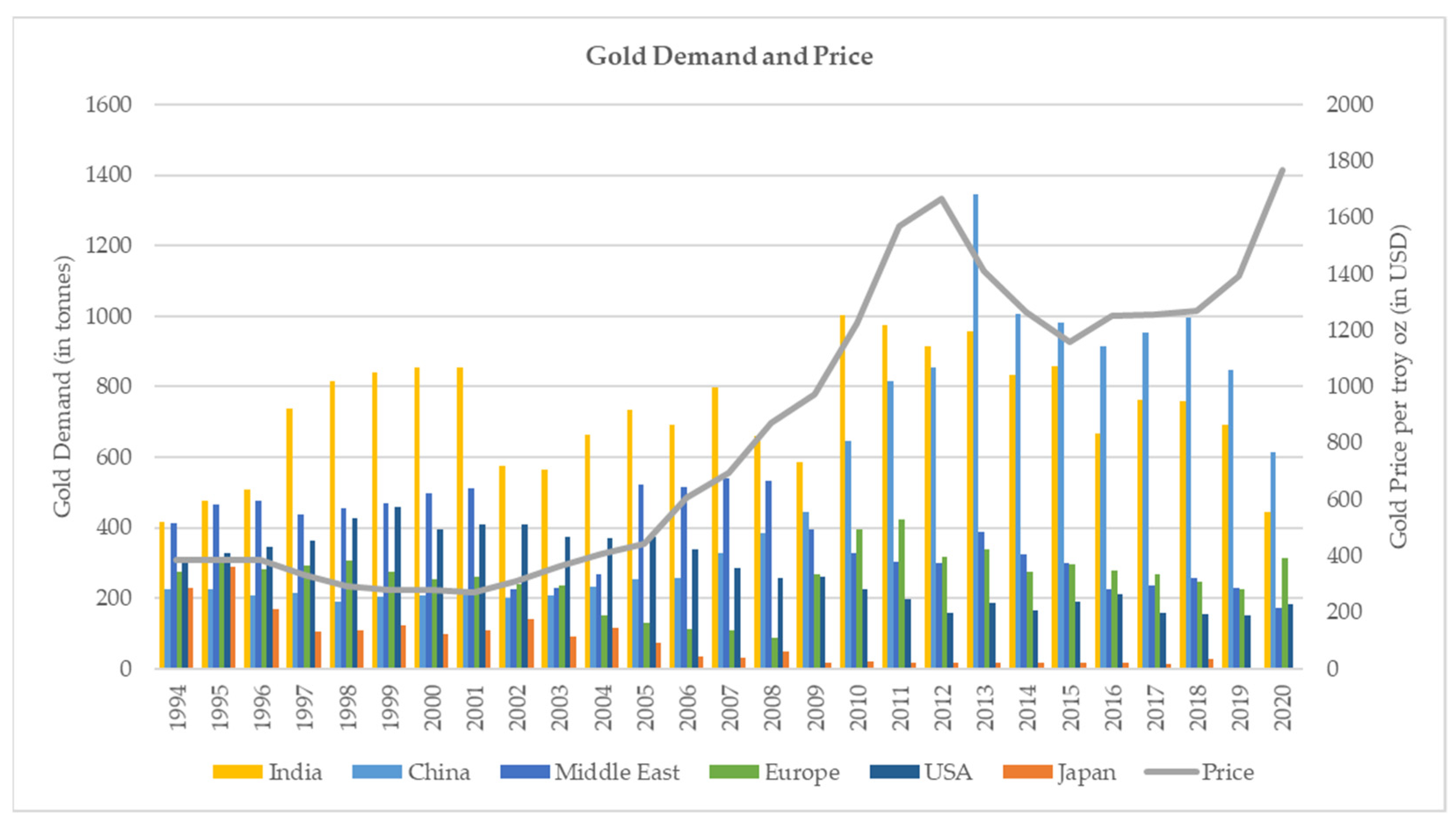
4.1. Trend in Gold Demand and Price

The relationship between gold demand and the price of all the countries included in the sample is exhibited in Figure 1.

Figure 1 shows that until 2012, India was the number one consumer of gold in the international market, after which it has become the second-largest consumer. During the study period, India’s average gold consumption per annum was around 180 tonnes. We also observe that there is an inverse relationship between the gold price and gold demand. When the price increases, the demand decreases, and vice versa. Until 2008, Middle Eastern countries were the second-largest consumer. From 2009 onwards, China became the second-largest consumer of gold and, subsequently, it occupied the first position since 2013.

4.2. Descriptive Statistics

The basic information about the variables included in the study is summarized in

Table 1. Descriptive statistics of the variables.

	Price		Demand
	AM Price	PM Price	India	China	Middle East	Europe	USA	Japan
Mean	834.29	834.04	181.85	129.47	92.77	64.44	71.36	18.12
Standard Error	48.67	48.65	5.49	8.81	3.12	2.73	3.07	1.82
Median	674.08	674.18	184.25	78.70	87.89	64.13	64.85	8.10
Mode			174.10	46.00	117.40	102.20	70.70	26.50
Standard Deviation	505.76	505.62	57.05	91.55	32.46	28.40	31.90	18.91
Sample Variance	255,792.44	255,649.50	3254.61	8382.26	1053.65	806.55	1017.91	357.57
Kurtosis	−1.34	−1.34	−0.20	0.58	−0.68	−0.10	0.56	1.88
Skewness	0.37	0.37	0.12	1.01	0.37	0.23	0.95	1.45
Range	1652.62	1652.19	286.97	442.71	154.51	120.80	138.19	90.02
Minimum	259.20	259.17	34.70	39.40	23.09	13.00	29.41	−3.62
Maximum	1911.82	1911.36	321.67	482.11	177.60	133.80	167.60	86.40
Count	108.00	108.00	108.00	108.00	108.00	108.00	108.00	108.00

.

The results reveal that average demand during the study period is highest for India, followed by China. The skewness is positive and near zero for India, and for other countries data have a slight variation. The positive skewness shows that there always exists a minimum amount of demand for gold.

4.3. Stationarity of the Variables

Unit root tests such as ADF (Dickey and Fuller 1979), (Dickey and Fuller 1981) and PP (Phillips and Perron 1988), (Phillips and Ouliaris 1990) tests are applied to find the stationarity of the variables and the results are shown in

Table 2. Stationarity of variables during different study periods.

Variables	Level		First Difference
	ADF	PP	ADF	PP
AM	0.052462	0.029757	−7.783063 *	−7.924205 *
	[0.9605]	[0.9586]	[0.0000]	[0.0000]
PM	0.056695	0.028996	−7.813382 *	−7.963598 *
	[0.9609]	[0.9585]	[0.0000]	[0.0000]
INDIA	−0.070992	−2.923395	−6.652775 *	−3.622162 **
	[0.6583]	[0.1566]	[0.0000]	[0.0296]
EUROPE	−2.629712	−1.525254	−4.976002 *	−4.791342 *
	[0.2674]	[0.5703]	[0.0003]	[0.0000]
CHINA	−1.826870	0.072792	−6.030721 *	−2.897450 *
	[0.6892]	[0.7052]	[0.0000]	[0.0038]
USA	−2.900411	−0.979818	−5.112069 *	−5.152639 *
	[0.1640]	[0.2926]	[0.0002]	[0.0000]
JAPAN	−2.192246	−2.056606	−12.67683 *	−17.87531 *
	[0.2097]	[0.2627]	[0.0000]	[0.0001]
MEAST	−1.193273	−0.884538	−4.999767 *	−3.893559 *
	[0.2129]	[0.3322]	[0.0000]	[0.0001]

Significance at * 1% level, ** 5% level, [ ] p values.

. The null hypothesis tested is that all the variables contain unit root at level or non-stationary against the alternative hypothesis that variables are stationary.

The results of both ADF and PP are highly significant for all the variables at the first difference. We accept the null hypothesis of non-stationary at the level. Hence, the unit root test results show that all the variables are integrated in the same order I(1).

4.4. Selection of VAR Lag Length

The inclusion of a suitable number of lags in the model makes it more meaningful to the results of the model. Whenever the VAR model is estimated, specifying the appropriate lag length is an important task, because it shows how long the changes in the variables should take to work through the system. The results of the VAR lag length selection based on the information criteria are given in

Table 3. Selection of VAR optimum lag length.

	Lag	LogL	LR	FPE	AIC	SC	HQ
AM	0	−10,251.20	NA	2.62 × 1022	71.48569	71.57494	71.52146
	1	−7678.774	5001.434	6.05 × 1014	53.90086	54.61491	54.18704
	2	−6676.761	1899.286	7.90 × 1011	47.25966	48.59849	47.79624
	3	−5856.521	1514.728	3.67 × 109	41.88516	43.84879	42.67216
	4	−5322.817	959.5518	1.25 × 108	38.50744	41.09585 *	39.54483
	5	−5217.193	184.7493 *	84,901,681 *	38.11285 *	41.32605	39.40065 *
PM	0	−10,250.95	NA	2.62 × 1022	71.48398	71.57324	71.51976
	1	−7677.415	5003.602	5.99 × 1014	53.89139	54.60544	54.17757
	2	−6675.179	1899.708	7.81 × 1011	47.24863	48.58747	47.78522
	3	−5855.270	1514.118	3.63 × 109	41.87645	43.84007	42.66344
	4	−5321.265	960.0930	1.24 × 108	38.49662	41.08503 *	39.53402
	5	−5215.803	184.4655 *	84,083,295 *	38.10316 *	41.31636	39.39096 *

* Indicates lag order selected by the criterion; LR: sequential modified LR test statistic (each test at 5% level); FPE: final prediction error; AIC: Akaike information criterion; SC: Schwarz information criterion; HQ: Hannan–Quinn information criterion.

. Selection of the lag length for all the variables is conducted based on the lag length suggested by the Schwarz Information criterion. Lag length is estimated separately for the dependent variables AM fix and PM fix prices.

4.5. Results of the Long-Run Relationship between Gold Demand and Prices

The results of the Johansen Cointegration test (Johansen 1988), (Johansen 1991), (Johansen and Juselius 1990) are given in

Table 4. Results of long-run relationship between the gold prices and gold demand.

Variable	Hypothesis	Eigen Value	Trace Statistics	Critical Value at 5%	Prob **	Max-Eigen Statistic	Critical Value at 5%	Prob **
AM Fix	r = 0 *	0.288116	222.9854	125.6154	0.0000	97.53422	46.23142	0.0000
	r ≤ 1 *	0.160338	125.4512	95.75366	0.0001	50.15485	40.07757	0.0027
	r ≤ 2 *	0.128852	75.29631	69.81889	0.0171	39.58982	33.87687	0.0093
	r ≤ 3	0.066035	35.70649	47.85613	0.4113	19.60667	27.58434	0.3690
	r ≤ 4	0.031220	16.09982	29.79707	0.7052	9.102895	21.13162	0.8240
	r ≤ 5	0.019506	6.996923	15.49471	0.5780	5.653435	14.26460	0.6580
	r ≤ 6	0.004670	1.343488	3.841466	0.2464	1.343488	3.841466	0.2464
PM Fix	r = 0 *	0.287561	223.4965	125.6154	0.0000	97.31038	46.23142	0.0000
	r ≤ 1 *	0.161508	126.1862	95.75366	0.0001	50.55522	40.07757	0.0024
	r ≤ 2 *	0.129868	75.63094	69.81889	0.0159	39.92458	33.87687	0.0084
	r ≤ 3	0.066076	35.70636	47.85613	0.4113	19.61936	27.58434	0.3681
	r ≤ 4	0.031166	16.08699	29.79707	0.7061	9.087066	21.13162	0.8253
	r ≤ 5	0.019504	6.999928	15.49471	0.5776	5.652982	14.26460	0.6581
	r ≤ 6	0.004682	1.346946	3.841466	0.2458	1.346946	3.841466	0.2458

Trace test indicates 2 cointegrating eqn(s) at the 0.05 level; * denotes rejection of the hypothesis at the 0.05 level; max-eigenvalue test indicates 1 cointegrating eqn(s) at the 0.05 level; ** MacKinnon–Haug–Michelis (1999) p-values.

. It is observed from the results that the Trace statistics and Max-Eigen statistics are significant at r = 0. It means we fail to accept the null hypothesis of which there is no cointegration. Hence, there exists a long-run relationship between gold prices and gold demand. This witnesses that the gold demand of all the countries move together in the long run.

4.6. Individual and Collective Impact of the Variables

The existence of the long-run relationship between the gold prices and demand allows us to further examine whether the demand shows any significant impact on the price fixation. When many lags of variables are included in a VAR, it is very difficult to identify which sets of variables show a significant effect on each dependent variable and which do not. In order to address this issue, a test is conducted by restricting all the lags of particular variables to zero. The impact of independent variables individually and collectively on the dependent variables is estimated through the VAR Granger Causality/Block Exogeneity Wald test and presented in

Table 5. Individual and collective impact of the independent variables on dependent variables.

Countries	AM	PM
China	11.46316 **	11.46697 **
	[0.0218]	[0.0218]
Europe	2.823325	2.676316
	[0.5878]	[0.6134]
India	14.26114 *	14.61548 *
	[0.0065]	[0.0056]
Middleast	0.985495	1.036224
	[0.9120]	[0.9043]
USA	1.097667	1.056319
	[0.8946]	[0.9011]
Japan	5.747930	5.559686
	[0.2188]	[0.2345]
All	39.73789 **	39.85663 **
	[0.0228]	[0.0222]

Chi-square values and [ ] p values; *, **, indicates the level of significance at 1% and 5% respectively.

.

This model is estimated to determine whether the lags of one variable Granger cause any other of the variables in the system. Under the Block exogeneity test, the lag of a variable is restricted by equating to zero in a system. This restriction will enable us to identify the impact of the unrestricted variable on the dependent variables. It is estimated separately for AM and PM fix prices.

It is illustrated from the results that the international gold price of LBMA AM and PM fix prices are significantly influenced by gold demand. Hence, we fail to accept the null hypothesis. The demand of all the countries together influences the world gold prices. The individual effect is observed only in India and China. The gold consumption of India (Rajalakshmi Nirmal and Lokeshwarri SK 2021) and China significantly influences both the prices of AM and PM fix. It further supports the statement made by Gabriel (2012), who stated that India’s gold demand exerts great effects on the gold price.

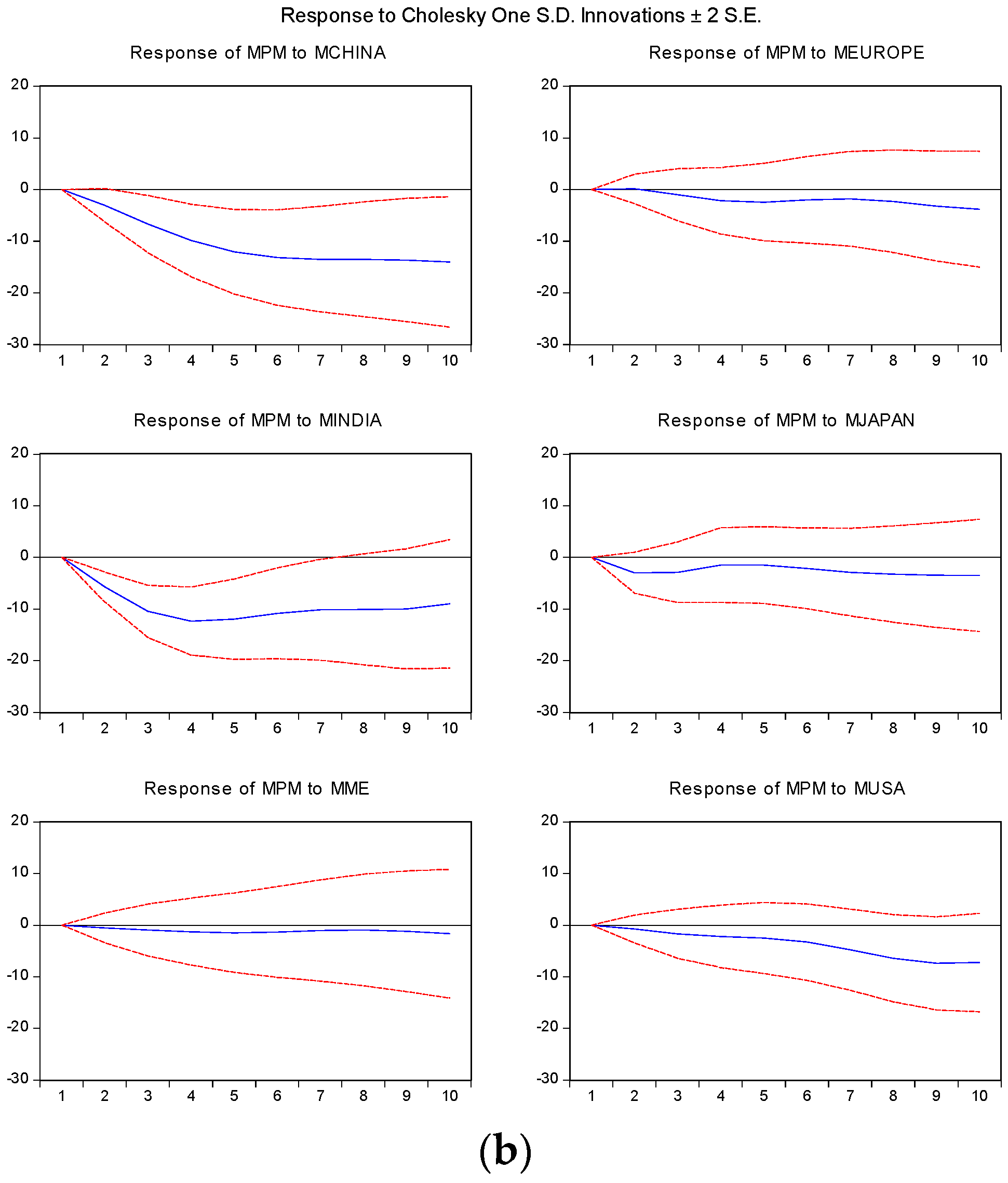
4.7. Transmission of Shocks—Impulse Response Function

The VAR Granger Causality/Block Exogeneity Wald test (GCBEW) provides only the significance level and does not provide the sign of how the shocks in exogenous variables are transmitted to the endogenous variable. The Impulse Response Function (IRF) captures this effect.

The results of the IRF are given in Figure 2. Figure 2a,b exhibit AM fix and PM fix, respectively. It is found from the graphs that both the prices immediately and negatively react to the shocks transmitted from India and China. The shocks sustain over a period of time and the system takes a long time to get back to equilibrium. The consumption of both China and India are able to cause disequilibrium both in AM and PM fix prices. The AM and PM prices’ reaction to the changes in demand in the Middle East is minuscule, as their deviation from the mean line is extremely small. AM and PM fix prices marginally react to the changes in the gold demand of the USA, Europe, and Japan. The effects on Japan and Europe are similar. However, the reaction to the changes in the USA demand is slow. In the long run, the deviation keeps increasing.

4.8. Proportion of Share of Variances

Variance Decomposition separates the variations in an endogenous variable into the component shocks to the VAR. It provides information about the proportion of variances that is transmitted to other variables in the system. The results given in

Table 6. The proportion of variances transmitted to AM and PM fix prices.

Period	S.E.	AM	CHINA	EUROPE	INDIA	JAPAN	ME	USA
1	32.87089	100.0000	0.000000	0.000000	0.000000	0.000000	0.000000	0.000000
2	48.83444	97.81736	0.369022	0.002640	1.362191	0.412170	0.011811	0.024805
3	60.28221	93.96896	1.437363	0.020277	3.916234	0.525709	0.030454	0.101004
4	70.57235	90.33201	2.960562	0.099475	5.935963	0.441409	0.052982	0.177601
5	80.51930	87.86119	4.492252	0.162236	6.792671	0.382519	0.072330	0.236802
6	89.94258	86.37892	5.747412	0.176895	6.918623	0.374386	0.079009	0.324757
7	98.76150	85.38511	6.643931	0.175779	6.807959	0.407142	0.076038	0.504037
8	107.0527	84.54426	7.249423	0.189330	6.695781	0.452383	0.071566	0.797257
9	114.8859	83.78750	7.694000	0.235001	6.589393	0.496272	0.071724	1.126109
10	122.2276	83.24309	8.091308	0.299486	6.385866	0.532952	0.080716	1.366585
Period	S.E.	PM	CHINA	EUROPE	INDIA	JAPAN	ME	USA
1	32.75884	100.0000	0.000000	0.000000	0.000000	0.000000	0.000000	0.000000
2	48.55616	97.78275	0.395436	0.000573	1.401004	0.384046	0.012659	0.023530
3	59.97487	93.85970	1.515672	0.028425	3.981353	0.488187	0.032664	0.094002
4	70.23423	90.17236	3.084398	0.118097	6.000755	0.402811	0.056110	0.165472
5	80.11301	87.68341	4.636716	0.183294	6.851640	0.345443	0.075958	0.223535
6	89.45171	86.20311	5.892530	0.198104	6.974789	0.335484	0.082777	0.313202
7	98.20075	85.22055	6.782923	0.197985	6.860249	0.364696	0.079898	0.493696
8	106.4393	84.39227	7.388850	0.214875	6.740564	0.405294	0.075625	0.782525
9	114.2289	83.64683	7.845735	0.265642	6.621410	0.444599	0.076329	1.099456
10	121.5296	83.10989	8.264412	0.333877	6.402074	0.477294	0.086176	1.326274

exhibit that most of the variances are explained by their own lagged shock in the short run. In the long run, India and China significantly transmit their shocks to AM and PM fix prices. The proportion of the variances is increasing in the long run. The variances transmitted from other major gold-consuming countries are extremely small, both in the short run as well as in the long run.

5. Conclusions

It is concluded from the empirical results that the international benchmark prices LBMA AM and PM fix prices are influenced by the gold demand of all the major gold-consuming countries. The LBMA fix prices and the gold demand of all the countries move together in the long run. In the long run, either demand or price can be used to analyse the behaviour of the other. Overall, the demand of all the countries together affects the price fluctuations. The individual effect is significant only for India (Rajalakshmi Nirmal and Lokeshwarri SK 2021) and China. The significance level is comparatively higher for India than for China. The demand of other countries did not have any significance in the analysis. Their volume of consumption in the world gold markets is not as significant as in India and China. The shock that arises in these two markets significantly affects the LBMA AM and PM fix prices in the long run, and furthermore, the quantity of variances accounted for continues to increase in the long run. These two countries’ demand is pivotal in the fixation of LBMA prices in the world gold markets. These countries do not fix their own price, but they derive the price from the international markets. The information available in these markets are highly leveraged in their price fixation. Hence, the study concludes that the volume of gold consumption significantly influences the international benchmark prices.

In spite of being the largest consumer of gold in the gold market, India is a price taker Kannan and Dhal (2008). Bullion associations and commodity exchanges that allow bullion trade in India may take initiatives to make India a price maker in the world gold markets. This will fulfil the dreams of many bullion traders in India. Investors, bullion traders, and banks can observe the gold consumption patterns of India and China to forecast the world gold price movements. This prediction could be helpful for them to minimize the risk involved in trading. It is strongly argued that in a scenario of the destruction of the paper gold market, ownership of physically allocated and segregated gold is paramount. If the paper gold bubble bursts, physical gold ownership is the only thing that can protect against a systemic collapse of the financial system and protect against the destruction of the fractionally reserved gold banking system (BullionStar 2017b). Gold price set by the derivatives market has destroyed the price of gold without any physical gold involved (Aasif 2018). Hence, it is safer to follow the price set by the physical markets than the paper market in gold.

References

1. Aasif, Hirani. 2018. Who Sets Gold Price? This Will Change Your Outlook for the Yellow Metal. Available online: https://economictimes.indiatimes.com/markets/commodities/views/who-sets-gold-price-this-will-change-your-outlook-for-the-yellow-metal/articleshow/62365567.cms?from=mdr (accessed on 20 December 2021).
2. Bahmani-Oskooee, Mohsen. 1987. Effects of Rising Price of Gold on the LDSs’ Demand for International Reserves. International Economic Journal 1: 35–44. [Google Scholar] [CrossRef]
3. Batchelor, Roy, and David Gulley. 1995. Jewellery demand and the price of gold. Resources Policy 21: 37–42. [Google Scholar] [CrossRef]
4. Bhattacharya, Himadri. 2002. Deregulation of Gold in India: A Case Study in Deregulation of a Gold Market. Research Study No. 27. London: World Gold Council: Research Study, pp. 1–28. [Google Scholar]
5. BullionStar. 2017a. What Sets the Gold Price? Is It the Paper Market or Physical Market? Available online: https://www.bullionstar.com/blogs/bullionstar/what-sets-the-gold-price-is-it-the-paper-market-or-physical-market/ (accessed on 20 December 2021).
6. BullionStar. 2017b. Indian Gold Market. Available online: https://www.bullionstar.com/gold-university/indian-gold-market (accessed on 15 December 2021).
7. Dan Popescu. 2014. India’s Role in the Gold Market. Available online: https://goldbroker.com/news/india-major-player-gold-market-519 (accessed on 1 March 2022).
8. Dickey, David, and Wayne A. Fuller. 1979. Distribution of Estimators for Time Series Regressions with a Unit Root. Journal of the American Statistical Association 74: 427–31. [Google Scholar]
9. Dickey, David A., and Wayne A. Fuller. 1981. Likelihood Ratio Statistics for Autoregressive Time Series with a Unit Root. Econometrica 49: 1057–72. [Google Scholar] [CrossRef]
10. Faugere, Christophe, and Julian Van Erlach. 2005. The Price of gold: A global required yield theory. The Journal of Investing 14: 99–111. [Google Scholar] [CrossRef]
11. Gabriel, M. Muller. 2012. Asian Gold Demand: Key Price Determinant. Available online: http://www.resourceinvestor.com/2012/08/09/asian-gold-demand-key-price-determinant (accessed on 20 December 2021).
12. Govett, M. H., and G. J. S. Govett. 1982. Gold demand and supply. Resource Policy 8: 84–96. [Google Scholar] [CrossRef]
13. Hauptfleisch, Martin, Tālis J. Putniņš, and Brian Lucey. 2016. Who Sets the Price of Gold? London or New York. The Journal of Futures Market 36: 564–86. [Google Scholar] [CrossRef] [Green Version]
14. Jena, Sangram Keshari, Aviral Kumar Tiwari, and David Roubaud. 2018. Comovements of gold futures markets and the spot market: A wavelet analysis. Finance Research Letters 24: 19–24. [Google Scholar] [CrossRef]
15. Johansen, Søren. 1988. Statistical Analysis of Cointegrating Vectors. Journal of Economic Dynamics and Control 12: 231–54. [Google Scholar] [CrossRef]
16. Johansen, Søren. 1991. Estimation and hypothesis testing of cointegration vectors in Gaussian vector autoregressive models. Econometrica 59: 1551–80. [Google Scholar] [CrossRef]
17. Johansen, Soren, and Katarina Juselius. 1990. Maximum Likelihood Estimation and Inference on Cointegration with Applications to the Demand for Money. Oxford Bulletin of Economics and Statistics 52: 169–210. [Google Scholar] [CrossRef]
18. Kannan, R., and Sarat Dhal. 2008. India’s Demand for Gold: Some Issues for Economy Development and Macroeconomic Policy. Indian Journal of Economics & Business 7: 107–28. [Google Scholar]
19. Lin, Min, Gang-Jin Wang, Chi Xie, and H. Eugene Stanley. 2018. Cross-correlations and influence in world gold markets. Physica A: Statistical Mechanics and Its Applications 490: 504–12. [Google Scholar] [CrossRef]
20. Lucey, Brian M., Charles Larkin, and Fergal A. O’Connor. 2013. London or New York: In which does the gold price originate and when? Applied Economics Letters 20: 813–17. [Google Scholar] [CrossRef] [Green Version]
21. Lucey, Brian M., Charles Larkin, and Fergal O’Connor. 2014. Gold Markets Around the World—Who Spills Over What, to Whom, When? Applied Economics Letters 21: 887–92. [Google Scholar] [CrossRef]
22. MacKinnon, James G., Alfred A. Haug, and Leo Michelis. 1999. Numerical Distribution Functions of Likelihood Ratio Tests for Cointegration. Journal of Applied Econometrics 14: 563–77. [Google Scholar] [CrossRef]
23. O’Connor, Fergal A., Brian M. Lucey, Jonathan A. Batten, and Dirk G. Baur. 2015. The Financial Economics of Gold—A Survey. International Review of Financial Analysis 41: 186–205. [Google Scholar] [CrossRef]
24. Ong, E., M. Grubb, and A. Mitra. 2009. India: Heart of Gold Strategic Outlook. London: World Gold Council. [Google Scholar]
25. Ong, E., J. C. Artigas, J. Palmberg, L. Street, N. Tuteja, and M. Grubb. 2010. India: Heart of Gold Revival. London: World Gold Council. [Google Scholar]
26. Patel, I. G., and Anand Chandavarkar. 2006. India’s Elasticity of Demand for Gold. Economic and Political Weekly 41: 507–16. [Google Scholar]
27. Phillips, Peter C. B., and Sam Ouliaris. 1990. Asymptotic properties of residual based tests for cointegration. Econometrica 58: 165–93. [Google Scholar] [CrossRef] [Green Version]
28. Phillips, Peter C. B., and Pierre Perron. 1988. Testing for a unit root in time series regressions. Biometrika 75: 335–46. [Google Scholar] [CrossRef]
29. Radetzki, Marian. 1989. The fundamental determinants of their price behaviour. Resources Policy 15: 194–208. [Google Scholar] [CrossRef]
30. Rajalakshmi Nirmal and Lokeshwarri SK. 2021. Opinion: India Must Be a Metal Price Setter Globally. Available online: https://www.thehindubusinessline.com/opinion/india-must-be-a-metal-price-setter-globally/article25550372.ece (accessed on 15 January 2022).
31. Selvanathan, Saroja, and E. A. Selvanathan. 1999. The effect of the price of gold on its production: A time-series analysis. Resources Policy 25: 265–75. [Google Scholar] [CrossRef]
32. Shafiee, Shahriar, and Erkan Topal. 2010. An overview of global gold market and gold price forecasting. International Journal of Minerals Policy and Economics 35: 178–89. [Google Scholar] [CrossRef]
33. Starr, Martha, and Ky Tran. 2008. Determinants of the Physical Demand for Gold: Evidence from Panel Data. The World Economy 31: 416–36. [Google Scholar] [CrossRef]
34. Warren, G. F., and F. A. Pearson. 1933. Relationship of Gold to Prices. In Proceedings of the American Statistical Association, supplement. Journal of the American Statistical Association 28: 118–26. [Google Scholar]
35. Xu, Xiaoqing Eleanor, and Hung-Gay Fung. 2005. Cross-market linkages between U.S. and Japanese precious metals futures trading. Journal of International Financial Markets, Institutions & Money 15: 107–24. [Google Scholar]
36. Yurdakul, Funda, and Merve Sefa. 2015. An Econometric Analysis of Gold Prices in Turkey. Procedia Economics and Finance 23: 77–85. [Google Scholar] [CrossRef] [Green Version]
Figure 1. International gold price and demand trend.
Jrfm 15 00273 g001
Figure 2. Transmission of shocks of price on AM Fix (a) and PM Fix prices (b).
Jrfm 15 00273 g002aJrfm 15 00273 g002b