Monte Carlo Sensitivities Using the Absolute Measure-Valued Derivative Method

Abstract

Measure-valued differentiation (MVD) is a relatively new method for computing Monte Carlo sensitivities, relying on a decomposition of the derivative of transition densities of the underlying process into a linear combination of probability measures. In computing the sensitivities, additional paths are generated for each constituent distribution and the payoffs from these paths are combined to produce sample estimates. The method generally produces sensitivity estimates with lower variance than the finite difference and likelihood ratio methods, and can be applied to discontinuous payoffs in contrast to the pathwise differentiation method. However, these benefits come at the expense of an additional computational burden. In this paper, we propose an alternative approach, called the absolute measure-valued differentiation (AMVD) method, which expresses the derivative of the transition density at each simulation step as a single density rather than a linear combination. It is computationally more efficient than the MVD method and can result in sensitivity estimates with lower variance. Analytic and numerical examples are provided to compare the variance in the sensitivity estimates of the AMVD method against alternative methods.

1. Introduction

Sensitivities play a key role in the assessment and the management of risks associated with financial derivatives and must be computed along with prices as part of sound risk management practice. Given that it is not possible to compute the sensitivities let alone the prices of  many financial derivatives analytically, they are usually computed numerically, with Monte Carlo simulation being the most widely used technique. The associated sensitivities are then computed by finite difference, pathwise differentiation, or likelihood ratio methods, each with its own set of limitations. In particular, the finite difference method is biased and sensitivity estimates have relatively large variances, the pathwise derivative method cannot be applied to products with discontinuous payoffs such as digitals, and the likelihood ratio method can be subject to unbounded variance when the associated score function is not absolutely continuous with respect to the sensitivity parameter. For a detailed discussion of these methods and their limitations, refer to Glasserman (2004), chapter 7.

There has been extensive work on regularizing the pathwise method to enable it to work with discontinuities. Such work tends either to involve differentiating the discontinuity directly, which yields a delta distribution, or to utilize smoothing to avoid this differentiation. Joshi and Kainth (2004), Rott and Fries (2005), and Brace (2007) explore the explicit integration of the delta distribution, which requires at least one extra simulation that must be handcrafted to the payoff. Liu and Hong (2011) and Lyuu and Teng (2011) reduce the degree of handcrafting by employing kernel smoothing and importance sampling, respectively. Chan and Joshi (2015) modify the simulation scheme as a function of the perturbation variable so that the pathwise payoff, as a function of perturbation size, is smooth. It is then possible to apply the pathwise method at the cost of gaining a small likelihood ratio term. All these methods have the drawback that the methodology is adapted to the singularities of the payoff. This renders them much harder to implement generically than the likelihood ratio and pathwise methods.

Despite their importance, there is a relative absence of new techniques for computing Monte Carlo sensitivities, and recent advances have focused instead on improving the computational efficiency of existing techniques. For example, Capriotti and Giles (2018) apply adjoint algorithmic differentiation to speed up pathwise sensitivity calculations, while Xiang and Wang (2022) apply low discrepancy sequences to achieve variance reduction for American option sensitivities.

A notable exception is the measure-valued differentiation (MVD) method considered, for example, in Heidergott et al. (2008) and  Pflug and Thoma (2016). The MVD method does not differentiate the payoff and so discontinuities do not cause difficulties, and it has been shown to produce sensitivity estimates with lower variance than those computed using the finite difference and the likelihood ratio (LR) methods. It is also generic in the sense that it is not adapted to the payoff in any way, and so the same paths can be used to compute the sensitivities of many derivatives on the same underlying framework. In the MVD approach, the derivative of the transition density is recognized as a signed measure and decomposed as the difference of two proper measures. The simulation at each step is then branched according to the two constituent measures to produce multiple MVD paths. Sensitivity estimates from these branched paths are then recombined to produce one MVD sensitivity sample. It is shown that this approach generally results in sensitivity estimates with lower variance than alternative methods, albeit at the expense of a greater computational burden due to the branching of the paths. Further variance reduction is possible by coupling, or correlating, each pair of the branched paths.

In this paper, we introduce an alternative to the MVD method, called the absolute measure-valued differentiation (AMVD) method, which decomposes the density derivative as the product of its sign and its absolute value. This method shares many of the properties of the MVD method, such as the ability to handle discontinuous payoffs, but  instead of initiating two additional paths at each simulation step of the original path, it initiates only one additional subpath. It is found that the AMVD method gives vega estimates with lower variance than the MVD method for vanilla and digital calls in the Black–Scholes model. Moreover, the AMVD vega estimates have lower variance than the pathwise differentiation method in certain situations, such as the case of short-dated deep in-the-money vanilla calls. A consideration of vegas for the more exotic double-barrier options revealed that the relative performances of the LR, MVD, and AMVD methods depend, in general, on the positions of the barriers and the way each method distributes densities relative to the barriers.

Applying the AMVD method requires the generation of nonstandard random variates,1 and for the examples considered in this paper, we provide a highly efficient implementation of the inverse transform method for this purpose using Newton’s method with a careful selection of the initial point. The time taken to generate each vega subpath for the AMVD method is approximately equal to the time taken to generate the corresponding MVD method using the efficient generation of the double-sided Boltzmann–Maxwell distribution introduced in Heidergott et al. (2008).

The remainder of the paper is structured as follows: the measure-valued differentiation method is briefly reviewed in Section 2, and the absolute measure-valued differentiation method is presented in Section 3. This is followed by Section 4 in which the notation and key identities for the remainder of the paper are presented. Sensitivities for vanilla calls and digital calls are computed analytically in Section 5 and Section 6, respectively. A more complex example of the double knock-out barrier option is investigated numerically in Section 7, and the paper concludes with Section 8.

2. Brief Review of Measure-Valued Differentiation

In this section, we provide a heuristic overview of the MVD method and refer the interested reader to Heidergott et al. (2008) and Pflug and Thoma (2016) for the details.

Let X be an $\mathbb{R}$-valued random variable, and let $\varphi (x;\theta )$ be the probability density function of X with $\theta$ as one of its parameters. Then, given a payoff, $f:\mathbb{R}\to \mathbb{R}$, associated with a financial derivative on X, the likelihood ratio (LR) sensitivity with respect to the parameter $\theta$ is given by

$$\begin{array}{c}\hfill {\Delta }_{\theta }\left(f\right)={\int }_{\mathbb{R}}f\left(x\right)\frac{\partial \varphi (x;\theta )}{\partial \theta }dx\end{array}$$

(1)

ignoring discounting. At this point, the likelihood ratio method rewrites the above expression as

$$\begin{array}{c}\hfill {\Delta }_{\theta }^{\mathrm{LR}}\left(f\right)={\int }_{\mathbb{R}}\frac{\partial ln\varphi (x;\theta )}{\partial \theta }f\left(x\right)·\varphi (x;\theta )dx,\end{array}$$

(2)

and computes the sensitivity as the expectation of the modified payoff obtained by scaling $f\left(x\right)$ by the score function $\partial ln\varphi (x;\theta )/\partial \theta$.

Now, suppose $\phi \left(x\right)=\partial \varphi (x;\theta )/\partial \theta$ is a signed measure on $\mathbb{R}$, and that it decomposes as the difference

$$\begin{array}{c}\hfill \phi \left(x\right)={\phi }_1\left(x\right)-{\phi }_2\left(x\right),\end{array}$$

(3)

where ${\phi }_1$ and ${\phi }_2$ are proper measures on $\mathbb{R}$. Then, under the MVD method, the sensitivity with respect to $\theta$ is computed as the difference

$$\begin{array}{c}\hfill {\Delta }_{\theta }^{\mathrm{MVD}}\left(f\right)=\mu \left({\phi }_1\right){\int }_{\mathbb{R}}f\left(x\right)\frac{{\phi }_1\left(x\right)}{\mu \left({\phi }_1\right)}dx-\mu \left({\phi }_2\right){\int }_{\mathbb{R}}f\left(x\right)\frac{{\phi }_2\left(x\right)}{\mu \left({\phi }_2\right)}dx,\end{array}$$

(4)

where $\mu \left({\phi }_i\right)={\int }_{\mathbb{R}}{\phi }_i\left(x\right)dx>0$. The two summands are computed separately, although they may be coupled to reduce the total variance. It should be noted that ${\overline{\phi }}_i\left(x\right)={\phi }_i\left(x\right)/\mu \left({\phi }_i\right)$, for $1\le i\le 2$, are probability measures on $\mathbb{R}$, and so the decomposition in (4) provides the basis for a numerical approximation of the sensitivity using, for example, a Monte Carlo simulation in which the integrals in (4) are computed numerically using random draws from the distributions determined by ${\overline{\phi }}_i\left(x\right)$.

The above description of the MVD method applies to path-independent European derivatives. For the more general case, suppose that a Monte Carlo simulation, with simulation times $0=t_0<t_1<\cdots <t_n=T$, is used to value a given derivative with expiry T. If the underlying process is assumed to be Markovian, then the probability density of a simulated path is given by the product

$$\begin{array}{c}\hfill \varphi (x_0,x_1,\dots ,x_n;\theta )=\prod _{i=1}^n{\varphi }_i(x_i\mid x_{i-1};\theta ),\end{array}$$

(5)

where ${\varphi }_i(x_i\mid x_{i-1};\theta )$ is the transition density from the $t_{i-1}$ to $t_i$ conditional starting from $x_{i-1}$ at $t_{i-1}$. For notational convenience, write $\varphi (\mathit{x};\theta )=\varphi (x_0,x_1,\dots ,x_n;\theta )$, ${\varphi }_i(x_i;\theta )={\varphi }_i(x_i\mid x_{i-1};\theta )$, and define

$$\begin{array}{c}\hfill {\partial }_{i,\theta }\varphi (\mathit{x};\theta )={\varphi }_1(x_1;\theta )\cdots {\varphi }_{i-1}(x_{i-1};\theta )\frac{\partial {\varphi }_i(x_i;\theta )}{\partial \theta }{\varphi }_{i+1}(x_{i+1};\theta )\cdots {\varphi }_n(x_n;\theta )\end{array}$$

(6)

The likelihood ratio sensitivity of a general payoff, $f\left(\mathit{x}\right)=f(x_0,x_1,x_2,\dots ,x_n)$, with  respect to the parameter, $\theta$, is then given by

$$\begin{array}{c}\hfill {\Delta }_{\theta }^{\mathrm{LR}}\left(f\right)=\sum _{i=1}^n{\int }_{{\mathbb{R}}^n}f\left(\mathit{x}\right){\partial }_{i,\theta }\varphi (\mathit{x};\theta )d\mathit{x}.\end{array}$$

(7)

Once again, if it is assumed that the derivatives

$$\begin{array}{c}\hfill {\phi }_i\left(x_i\right)=\frac{\partial {\varphi }_i(x_i,\theta )}{\partial \theta }\end{array}$$

(8)

are signed measures on $\mathbb{R}$, and decompose as differences

$$\begin{array}{c}\hfill {\phi }_i\left(x_i\right)={\phi }_{i,1}\left(x_i\right)-{\phi }_{i,2}\left(x_i\right),\end{array}$$

(9)

where ${\phi }_{i,j}\left(x\right)$ are proper measures, then the MVD estimate of the sensitivity is given by

$$\begin{array}{c}\hfill {\Delta }_{\theta }^{\mathrm{MVD}}\left(f\right)=\sum _{i=1}^n{\int }_{{\mathbb{R}}^n}f\left(\mathit{x}\right){\partial }_{i,\theta }^{\mathrm{MVD}}\varphi (\mathit{x};\theta )d\mathit{x},\end{array}$$

(10)

where ${\partial }_{i,\theta }^{\mathrm{MVD}}\varphi (\mathit{x};\theta )$ is obtained from ${\partial }_{i,\theta }(\mathit{x};\theta )$ by substituting the derivative term, $\partial {\varphi }_i(x_i;\theta )/\partial \theta$, in  (6) with its decomposition

$$\begin{array}{c}\hfill \frac{\partial {\varphi }_i(x_i;\theta )}{\partial \theta }=\mu \left({\phi }_{i,1}\right)\frac{{\phi }_{i,1}\left(x_i\right)}{\mu \left({\phi }_{i,1}\right)}-\mu \left({\phi }_{i,2}\right)\frac{{\phi }_{i,2}\left(x_i\right)}{\mu \left({\phi }_{i,2}\right)},\end{array}$$

(11)

where $\mu \left({\phi }_{i,j}\right)={\int }_{\mathbb{R}}{\phi }_{i,j}\left(x_i\right)d{x}_i$.

The implementation of the MVD method begins with the simulation, in the usual manner, of the underlying asset price path. Then, for each $1\le i\le n$, the i-th step is branched into two by drawing from distributions corresponding to the probability densities, ${\overline{\phi }}_{i,j}\left(x\right)={\phi }_{i,j}\left(x\right)/\mu \left({\phi }_{i,j}\right)$, for $1\le j\le 2$. The remaining steps in the two branched paths are then resimulated by drawing from the original distributions, ${\varphi }_j(x_j;\theta )$ for $i+1\le j\le n$. Thus, the full MVD method generates a set of $2n$ paths for each regular path and is consequently more computationally intensive than, for  example, the likelihood ratio method.2 In Pflug and Thoma (2016), less computationally demanding approximations to the full MVD method are proposed in which branching is performed only in a small subset of the simulation steps.

3. Absolute Measure-Valued Differentiation

An important factor taken into consideration when deciding on the form of the decomposition of the transition density in (9) is the additional computation burden associated with the need to generate random variates from the component distributions. The decomposition chosen in Heidergott et al. (2008) and Pflug and Thoma (2016) is due, at least in part, to ensuring that one of the components coincides with the distribution already used in generating the underlying process. The remaining factor, however, will generally be from a different distribution.

The main motivation behind the absolute measure-valued differentiation (AMVD) method is improve the computational efficiency of the MVD method by requiring the introduction of only one additional distribution and branching off only one path at each simulation step, while retaining the key features of the MVD method, viz., not requiring the payoff derivative, and producing sensitivity estimates with low variances. Using the notation from the previous section, the AMVD estimate for the sensitivity of a payoff f with respect to the parameter $\theta$ is defined by   

$$\begin{array}{c}\hfill {\Delta }_{\theta }^{\mathrm{AMVD}}\left(f\right)=\sum _{i=1}^n{\int }_{{\mathbb{R}}^n}f\left(\mathit{x}\right)\epsilon \left({\phi }_i\left(x_i\right)\right)\mu \left(|{\phi }_i|\right)\frac{{\partial }_{\left|i\right|,\theta }^{\mathrm{MVD}}\varphi (\mathit{x};\theta )}{\mu \left(|{\phi }_i|\right)}d\mathit{x},\end{array}$$

(12)

where $\epsilon \left({\phi }_i\left(x_i\right)\right)={\mathbf{1}}_{\{{\phi }_i\left(x_i\right)\ge 0\}}-{\mathbf{1}}_{\{{\phi }_i\left(x_i\right)<0\}}$, $\mu \left(|{\phi }_i|\right)={\int }_{\mathbb{R}}\left|{\phi }_i\left(x_i\right)\right|d{x}_i$, and 

$$\begin{array}{cc}\hfill {\partial }_{\left|i\right|,\theta }^{\mathrm{MVD}}\varphi (\mathit{x};\theta )& ={\varphi }_1(x_1;\theta )\cdots {\varphi }_{i-1}(x_{i-1};\theta )\left|{\phi }_i\left(x_i\right)\right|{\varphi }_{i+1}(x_{i+1};\theta )\cdots {\varphi }_n(x_n;\theta ).\hfill \end{array}$$

(13)

It follows from $\epsilon \left({\phi }_i\left(x_i\right)\right)\left|{\phi }_i\left(x_i\right)\right|={\phi }_i\left(x_i\right)$ that ${\Delta }_{\theta }^{\mathrm{AMVD}}\left(f\right)$ is an unbiased estimator for ${\Delta }_{\theta }\left(f\right)$. Moreover, although the AMVD method introduces what appears to be a problematic term, viz., $\epsilon \left({\phi }_i\left(x_i\right)\right)$, since $\epsilon \left({\phi }_i\left(x_i\right)\right)=\pm 1$, and these terms are squared when computing the associated variance, they do not adversely affect the AMVD variance.

4. Notation, Model, and Useful Identities

In situations where it applies, the pathwise differentiation (PW) method usually gives sensitivity estimates with lower variances than other methods, and it was shown in Pflug and Thoma (2016) that the MVD sensitivities have lower variance than the corresponding finite difference estimates. In subsequent sections, we will compare the variances of sensitivity estimates computed using the LR, MVD, AMVD, and  PW methods. Although the analysis could be performed for any sensitivity and with any underlying model, we will focus on delta and vega under the Black and Scholes (1973) model. This allows us to obtain, analytically, the variances of deltas and vegas for vanillas and digitals, and avoid the consideration of more complex models that do not contribute, in any substantial way, to the analysis of the relative performance of the various approaches for computing sensitivities.

4.1. Black–Scholes Delta and Vega

Let r be the risk-free rate, $S_t$ the price of the underlying asset at time t, and $\sigma$ the asset volatility. Moreover, let $0=t_0<t_1<\cdots <T_n=T$ be the sequence of Monte Carlo simulation times, and, for notational convenience, define

$$\begin{array}{c}\hfill S_i=S_{t_i},x_i=ln{S}_i,\mathrm{and}{\Delta }_j=t_{j+1}-t_j,\end{array}$$

(14)

where $0\le i\le n$ and $0\le j\le n-1$. The Euler–Maruyama discretization scheme for the Black–Scholes model

$$\begin{array}{c}\hfill x_{i+1}=x_i+\left(r-\frac{1}{2}{\sigma }^2\right){\Delta }_i+\sigma \sqrt{{\Delta }_i}{\xi }_i\end{array}$$

(15)

is unbiased, where ${\xi }_i\sim \mathcal{N}(0,1)$ is a normally distributed random variable. If we define

$$\begin{array}{c}\hfill {\mu }_i\left(\sigma \right)=\left(r-\frac{1}{2}{\sigma }^2\right){\Delta }_{i-1}\mathrm{and}{\varsigma }_i\left(\sigma \right)=\sigma \sqrt{{\Delta }_{i-1}},\end{array}$$

(16)

for $1\le i\le n$, then the transition density, ${\varphi }_i(x_i;\sigma )$, is given by

$$\begin{array}{c}\hfill {\varphi }_i(x_i;\sigma )=\frac{1}{{\varsigma }_i\left(\sigma \right)\sqrt{2\pi }}exp\left[-\frac{{\left(x_i-x_{i-1}-{\mu }_i\left(\sigma \right)\right)}^2}{2{\varsigma }_i^2\left(\sigma \right)}\right],\end{array}$$

(17)

so that $x_i\sim \mathcal{N}\left(x_{i-1}+{\mu }_i\left(\sigma \right),{\varsigma }_i^2\left(\sigma \right)\right)$. Straight-forward calculations give

$$\begin{array}{cc}\hfill {\phi }_1(x_i;S_0)& =\frac{\partial {\varphi }_1(x_1;S_0)}{\partial S_0}=\frac{1}{S_0{\varsigma }_1\left(\sigma \right)}{\xi }_1\varphi \left({\xi }_1\right),\hfill \end{array}$$

(18)

$$\begin{array}{cc}\hfill {\phi }_i(x_i;S_0)& =0,2\le i\le n,\hfill \end{array}$$

(19)

$$\begin{array}{cc}\hfill {\phi }_i(x_i;\sigma )& =\frac{\partial {\varphi }_i(x_i;\sigma )}{\partial \sigma }=\frac{1}{\sigma }\left({\xi }_i^2-{\varsigma }_i{\xi }_i-1\right)\varphi \left({\xi }_i\right),1\le i\le n,\hfill \end{array}$$

(20)

where ${\xi }_i$ is the standard normal random variate in (15) and $\varphi (·)$ is the standard normal density. The decompositions chosen for the MVD method in Pflug and Thoma (2016) are

$$\begin{array}{cc}\hfill {\phi }_1^{\mathrm{MVD}}(x_i;S_0)& =\frac{1}{S_0{\varsigma }_1\left(\sigma \right)}{\xi }_1\varphi \left({\xi }_1\right){\mathbf{1}}_{\{{\xi }_1\ge 0\}}-\frac{1}{S_0{\varsigma }_1\left(\sigma \right)}(-{\xi }_1)\varphi \left({\xi }_1\right){\mathbf{1}}_{\{{\xi }_1\le 0\}},\hfill \end{array}$$

(21)

$$\begin{array}{cc}\hfill {\phi }_i^{\mathrm{MVD}}(x_i;\sigma )& =\frac{1}{\sigma }{\xi }_i^2\varphi \left({\xi }_i\right)-\frac{{\varsigma }_i\left(\sigma \right)}{\sigma }{\xi }_i\varphi \left({\xi }_i\right){\mathbf{1}}_{\{{\xi }_i\ge 0\}}+\frac{{\varsigma }_i\left(\sigma \right)}{\sigma }(-{\xi }_i)\varphi \left({\xi }_i\right){\mathbf{1}}_{\{{\xi }_i\le 0\}}-\frac{1}{\sigma }\varphi \left({\xi }_i\right),\hfill \end{array}$$

(22)

where $2\le i\le n$. Both terms in (21) correspond to the density of the Rayleigh distribution, while in (22), the first term corresponds to the double-sided Maxwell–Boltzmann distribution, the second and third terms correspond to the Rayleigh distribution, and the last term is the standard normal density. Note that the linear terms in (18) and (20) were decomposed into two Rayleigh density terms since they define signed measures rather than proper measures on $\mathbb{R}$. The decompositions that will be used in the AMVD method are

$$\begin{array}{cc}\hfill {\phi }_1^{\mathrm{AMVD}}(x_i;S_0)& =\frac{1}{S_0{\varsigma }_1\left(\sigma \right)}\left|{\xi }_1\varphi \left({\xi }_1\right)\right|\varphi \left({\xi }_1\right),\hfill \end{array}$$

(23)

$$\begin{array}{cc}\hfill {\phi }_i^{\mathrm{AMVD}}(x_i;\sigma )& =\frac{1}{\sigma }\epsilon \left({\xi }_i^2-{\varsigma }_i\left(\sigma \right){\xi }_i-1\right)\left|{\xi }_i^2-{\varsigma }_i\left(\sigma \right){\xi }_i-1\right|\varphi \left({\xi }_i\right).\hfill \end{array}$$

(24)

4.2. Notation and Identities

For any $n\in {\mathbb{N}}_{+}$, define polynomials, $p_n\left(x\right)$, by $p_0\left(x\right)=1$ and for $n\ge 1$,

$$\begin{array}{c}\hfill p_n\left(x\right)=x^n-(n-1)x^{n-2}.\end{array}$$

(25)

Moreover, given any polynomial, $p\left(x\right)$, of degree n, and $a\in \mathbb{R}$, let ${\alpha }_i(p,a)\in \mathbb{R}$ be the coefficients in the decomposition

$$\begin{array}{c}\hfill p(x+a)=\sum _{i=0}^n{\alpha }_i(p,a)p_i\left(x\right),\end{array}$$

(26)

which are welldefined and unique since $\{p_i\left(x\right)\mid 0\le i\le n\}$ is a basis for the space of polynomials of degree at the highest n. For the purposes of computing the sensitivity variances, we note that

$$\begin{array}{c}\hfill {(x+a)}^2=1·\left(x^2-1\right)+2a·x+\left(a^2+1\right)·1,\end{array}$$

(27)

so that

$$\begin{array}{c}\hfill {\alpha }_0\left(x^2,a\right)=a^2+1,{\alpha }_1\left(x^2,a\right)=2a,\mathrm{and}{\alpha }_2\left(x^2,a\right)=1.\end{array}$$

(28)

If for any given $\zeta \in \mathbb{R}$, we define the quadratic $q_{\zeta }\left(x\right)$, by 

$$\begin{array}{c}\hfill q_{\zeta }\left(x\right)=x^2-\zeta x-1,\end{array}$$

(29)

then

$$\begin{array}{c}\hfill q_{\zeta }(x+a)=1·\left(x^2-1\right)+(2a-\zeta )·x+a(a-\zeta )·1,\end{array}$$

(30)

and so

$$\begin{array}{c}\hfill {\alpha }_0\left(q_{\zeta }\left(x\right),a\right)=a(a-\zeta ),{\alpha }_1\left(q_{\varsigma }\left(x\right),a\right)=2a-\zeta ,\mathrm{and}{\alpha }_2\left(q_{\varsigma }\left(x\right),a\right)=1.\end{array}$$

(31)

Next, squaring $q_{\zeta }\left(x\right)$ gives

$$\begin{array}{c}\hfill \begin{array}{cc}\hfill q_{\zeta }^2(x+a)& =1·\left(x^4-3x^2\right)+2\left(2a-\zeta \right)·\left(x^3-2x\right)\hfill \\ & +\left(6a^2-6\zeta a+{\zeta }^2+1\right)·\left(x^2-1\right)\hfill \\ & +\left(4a^3-6a^2\zeta +2a\left({\zeta }^2+2\right)-2\zeta \right)·x\hfill \\ & +\left(a^4-2\zeta a^3+\left({\zeta }^2+4\right)a^2-4\zeta a+{\zeta }^2+2\right)·1,\hfill \end{array}\end{array}$$

(32)

and so ${\alpha }_4\left(q_{\zeta }^2\left(x\right),a\right)=1$, ${\alpha }_3\left(q_{\zeta }^2\left(x\right),a\right)=2(2a-\zeta )$, and 

$$\begin{array}{cc}\hfill {\alpha }_0\left(q_{\zeta }^2\left(x\right),a\right)& =a^4-2\zeta a^3+\left({\zeta }^2+4\right)a^2-4\zeta a+{\zeta }^2+2,\hfill \end{array}$$

(33)

$$\begin{array}{cc}\hfill {\alpha }_1\left(q_{\zeta }^2\left(x\right),a\right)& =4a^3-6a^2\zeta +2a\left({\zeta }^2+2\right)-2\zeta ,\hfill \end{array}$$

(34)

$$\begin{array}{cc}\hfill {\alpha }_2\left(q_{\zeta }^2\left(x\right),a\right)& =6a^2-6\zeta a+{\zeta }^2+1.\hfill \end{array}$$

(35)

Finally, for any $i\in \mathbb{N}$, define

$$\begin{array}{c}\hfill {\chi }_i=(i-1)\vee 1=max\left(i-1,1\right),\end{array}$$

(36)

and given $a\in \mathbb{R}$, $l\le u\in \mathbb{R}$, and a polynomial $p\left(x\right)$ of degree n, define

$$\begin{array}{c}\hfill \begin{array}{cc}\hfill \mathcal{I}(p,a;l,u)& ={\alpha }_0(p,a)\left[\Phi \left(u-a\right)-\Phi \left(l-a\right)\right]\hfill \\ & +\varphi (l-a)\sum _{i=1}^n{\chi }_i{\alpha }_i(p,a){(l-a)}^{i-1}\hfill \\ & -\varphi (u-a)\sum _{i=1}^n{\chi }_i{\alpha }_i(p,a){(u-a)}^{i-1}.\hfill \end{array}\end{array}$$

(37)

In (37), we agree to set $\Phi (-\infty )=\varphi (\pm \infty )=0$ and $\Phi (\infty )=1$. Note that the definition of $\mathcal{I}(p,a;l,u)$ was motivated by the identity

$$\begin{array}{c}\hfill {\int }_l^u{e}^{ax}p\left(x\right)\varphi \left(x\right)dx=e^{\frac{1}{2}{a}^2}\mathcal{I}(p,a;l,u).\end{array}$$

(38)

It will be seen that the variances of deltas and vegas for vanilla and digital options can be obtained analytically and expressed succinctly in terms of $\mathcal{I}(p,a;l,u)$.

5. Vanilla Calls

For vanilla options, it is possible to derive analytic expressions for the variances of deltas and vegas for the LR, MVD, AMVD, and PW methods. We only provide the details for European calls, since the corresponding calculations for puts are entirely similar. Throughout this section, let K be the strike for a European call with expiry T, and let $\varsigma =\sigma \sqrt{T}$.

5.1. Vanilla Call Delta

Recall from (18) that if ${\Delta }_1=T$, then the derivative of the transition density from $t=0$ to $t=T$ with respect to $S_0$ is given by

$$\begin{array}{c}\hfill \phi (x_T;S_0)=\frac{\partial \varphi (x_T;S_0)}{\partial S_0}=\frac{1}{S_0\varsigma }\xi \varphi \left(\xi \right),\end{array}$$

(39)

where $\xi \sim \mathcal{N}(0,1)$, and for notational clarity, we have written $x_T=x_1$, $\xi ={\xi }_1$ and $\phi (x_T;S_0)={\phi }_1(x_1;S_0)$. The likelihood ratio estimator for the call delta is unbiased and computed using the expression   

$$\begin{array}{cc}\hfill \mathbb{E}\left[{\Delta }_{S_0}^{\mathrm{LR}}\left(c\right)\right]& ={\int }_{-{\xi }_{-}}^{\infty }\frac{e^{-rT}\xi }{S_0\varsigma }\left(S_0{e}^{\left(r-\frac{1}{2}{\sigma }^2\right)T+\varsigma \xi }-K\right)·\varphi \left(\xi \right)d\xi =\Phi \left({\xi }_{+}\right),\hfill \end{array}$$

where

$$\begin{array}{c}\hfill {\xi }_{\pm }=\frac{ln(S_0/K)+\left(r\pm \frac{1}{2}{\sigma }^2\right)T}{\varsigma }.\end{array}$$

(40)

The variance of the likelihood ratio call delta is given by

$$\begin{array}{c}\hfill \begin{array}{cc}\hfill \mathbb{V}\left[{\Delta }_{S_0}^{\mathrm{LR}}\left(c\right)\right]& =\frac{e^{{\varsigma }^2}}{{\varsigma }^2}\mathcal{I}\left(x^2,2\varsigma ;-{\xi }_{-},\infty \right)-\frac{2K{e}^{-rT}}{S_0{\varsigma }^2}\mathcal{I}\left(x^2,\varsigma ;-{\xi }_{-},\infty \right)\hfill \\ & +\frac{K^2{e}^{-2rT}}{S_0^2{\varsigma }^2}\mathcal{I}\left(x^2,0;-{\xi }_{-},\infty \right)-{\Phi }^2\left({\xi }_{+}\right).\hfill \end{array}\end{array}$$

(41)

The expected value of the MVD delta is unbiased and is computed using the expression

$$\begin{array}{cc}\hfill \mathbb{E}\left[{\Delta }_{S_0}^{\mathrm{MVD}}\left(c\right)\right]& ={\int }_{-{\xi }_{-}}^{\infty }\frac{e^{-rT}}{S_0\varsigma \sqrt{2\pi }}\left[S_0{e}^{\left(r-\frac{1}{2}{\sigma }^2\right)T+\varsigma \xi }-K\right]·{\mathbf{1}}_{\{\xi \ge 0\}}\sqrt{2\pi }\xi \varphi \left(\xi \right)d\xi \hfill \\ & -{\int }_{-{\xi }_{-}}^{\infty }\frac{e^{-rT}}{S_0\varsigma \sqrt{2\pi }}\left[S_0{e}^{\left(r-\frac{1}{2}{\sigma }^2\right)T+\varsigma \xi }-K\right]·{\mathbf{1}}_{\{\xi <0\}}\sqrt{2\pi }(-\xi )\varphi \left(\xi \right)d\xi ,\hfill \end{array}$$

where the terms are computed independently. The coefficient, $\sqrt{2\pi }$, preceding the terms $\pm \xi \varphi \left(\xi \right)$, is introduced to ensure that the product is a probability density function. The variance of the MVD delta is given by

$$\begin{array}{c}\hfill \mathbb{V}\left[{\Delta }_{S_0}^{\mathrm{MVD}}\left(c\right)\right]=m_{S_0}^{\left(2\right)}\left(c\right)-{\Phi }^2\left({\xi }_{-}\right),\end{array}$$

(42)

where

$$\begin{array}{c}\hfill \begin{array}{cc}\hfill m_{S_0}^{\left(2\right)}\left(c\right)& =\frac{e^{{\varsigma }^2}}{\sqrt{2\pi }{\varsigma }^2}\mathcal{I}\left(x,2\varsigma ;0\vee -{\xi }_{-},\infty \right)-\frac{2K{e}^{-rT}}{\sqrt{2\pi }{S}_0{\varsigma }^2}\mathcal{I}\left(x,\varsigma ;0\vee -{\xi }_{-},\infty \right)\hfill \\ & +\frac{K^2{e}^{-2rT}}{\sqrt{2\pi }{S}_0^2{\varsigma }^2}\mathcal{I}\left(x,0;0\vee -{\xi }_{-},\infty \right)-\frac{e^{{\varsigma }^2}}{\sqrt{2\pi }{\varsigma }^2}\mathcal{I}\left(x,2\varsigma ;0\wedge -{\xi }_{-},0\right)\hfill \\ & +\frac{2K{e}^{-rT}}{\sqrt{2\pi }{S}_0{\varsigma }^2}\mathcal{I}\left(x,\varsigma ;0\wedge -{\xi }_{-},0\right)-\frac{K^2{e}^{-2rT}}{\sqrt{2\pi }{S}_0^2{\varsigma }^2}\mathcal{I}\left(x,0;0\wedge -{\xi }_{-},0\right).\hfill \end{array}\end{array}$$

(43)

The expected value of the AMVD delta is unbiased and is computed using the expression

$$\begin{array}{c}\hfill \mathbb{E}\left[{\Delta }_{S_0}^{\mathrm{AMVD}}\left(c\right)\right]={\int }_{-{\xi }_{-}}^{\infty }\epsilon \left(\xi \right)\frac{e^{-rT}}{S_0\varsigma }\sqrt{\frac{2}{\pi }}\left[S_0{e}^{\left(r-\frac{1}{2}{\sigma }^2\right)T+\varsigma \xi }-K\right]·\sqrt{\frac{\pi }{2}}\left|\xi \right|\varphi \left(\xi \right)d\xi ,\end{array}$$

and its variance is given by

$$\begin{array}{c}\hfill \mathbb{V}\left[{\Delta }_{S_0}^{\mathrm{AMVD}}\left(c\right)\right]=2m_{S_0}^{\left(2\right)}\left(c\right)-{\Phi }^2\left({\xi }_{+}\right).\end{array}$$

(44)

It should be noted that although $\mathbb{V}\left[{\Delta }_{S_0}^{\mathrm{MVD}}\left(c\right)\right]$ is approximately half the value of $\mathbb{V}\left[{\Delta }_{S_0}^{\mathrm{AMVD}}\left(c\right)\right]$, implementing MVD using a Monte Carlo simulation would require two paths for each sample, while the AMVD method requires only one. Finally, the expected value for the PW delta is given by

$$\begin{array}{c}\hfill \mathbb{E}\left[{\Delta }_{S_0}^{\mathrm{PW}}\left(c\right)\right]={\int }_{-{\xi }_{-}}^{\infty }{e}^{-\frac{1}{2}{\varsigma }^2+\varsigma \xi }·\varphi \left(\xi \right)d\xi ,\end{array}$$

with the associated variance

$$\begin{array}{c}\hfill \mathbb{V}\left[{\Delta }_{S_0}^{\mathrm{PW}}\left(c\right)\right]=e^{{\varsigma }^2}\mathcal{I}\left(1,2\varsigma ;-{\xi }_{-},\infty \right)-{\Phi }^2\left({\xi }_{+}\right)=e^{{\varsigma }^2}\Phi \left({\xi }_{+}+\varsigma \right)-{\Phi }^2\left({\xi }_{+}\right).\end{array}$$

(45)

The ratios of variances for the vanilla call delta are shown in Figure 1 and Figure 2. It can be seen that the AMVD method gives lower variances than the LR method, but higher variances than the MVD method. Somewhat unexpectedly, the AMVD method results in lower variances than the PW method for short-dated deep in-the-money calls.

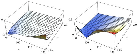
Figure 1. On the left, there is the ratio $\mathbb{V}\left[{\Delta }_{S_0}^{\mathrm{LR}}\left(c\right)\right]/\mathbb{V}\left[{\Delta }_{S_0}^{\mathrm{AMVD}}\left(c\right)\right]$ and, on the right, there is the ratio $\mathbb{V}\left[{\Delta }_{S_0}^{\mathrm{MVD}}\left(c\right)\right]/\mathbb{V}\left[{\Delta }_{S_0}^{\mathrm{AMVD}}\left(c\right)\right]$.

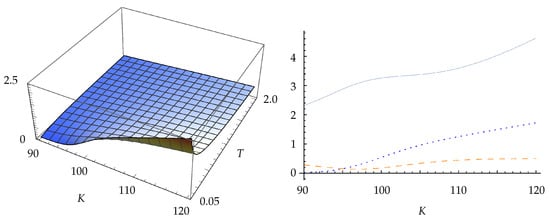
Figure 2. On the left, there is the ratio $\mathbb{V}\left[{\Delta }_{S_0}^{\mathrm{PW}}\left(c\right)\right]/\mathbb{V}\left[{\Delta }_{S_0}^{\mathrm{AMVD}}\left(c\right)\right]$. On the right, there are variance ratios at $T=0.1$. The solid curve is $\mathbb{V}\left[{\Delta }_{S_0}^{\mathrm{LR}}\left(c\right)\right]/\mathbb{V}\left[{\Delta }_{S_0}^{\mathrm{AMVD}}\left(c\right)\right]$, the dashed curve is $\mathbb{V}\left[{\Delta }_{S_0}^{\mathrm{MVD}}\left(c\right)\right]/\mathbb{V}\left[{\Delta }_{S_0}^{\mathrm{AMVD}}\left(c\right)\right]$, and the dotted curve is $\mathbb{V}\left[{\Delta }_{S_0}^{\mathrm{PW}}\left(c\right)\right]/\mathbb{V}\left[{\Delta }_{S_0}^{\mathrm{AMVD}}\left(c\right)\right]$.

5.2. Vanilla Call Vega

The derivative of the transition density, $\varphi (x_T;\sigma )$, with respect to $\sigma$ is given by

$$\begin{array}{c}\hfill \phi (x_T;\sigma )=\frac{\partial \varphi (x_T;\sigma )}{\partial \sigma }=\frac{1}{\sigma }\left({\xi }^2-\varsigma \xi -1\right)\varphi \left(\xi \right),\end{array}$$

(46)

where $\varsigma =\sigma \sqrt{T}$ is as defined previously. The likelihood ratio vega for the vanilla call is unbiased and is given by

$$\begin{array}{c}\hfill \mathbb{E}\left[{\Delta }_{\sigma }^{\mathrm{LR}}\left(c\right)\right]={\int }_{-{\xi }_{-}}^{\infty }\frac{e^{-rT}}{\sigma }\left[S_0{e}^{\left(r-\frac{1}{2}{\sigma }^2\right)T+\sigma \sqrt{T}\xi }-K\right]\left({\xi }^2-\varsigma \xi -1\right)·\varphi \left(\xi \right)d\xi ,\end{array}$$

so that $\mathbb{E}\left[{\Delta }_{\sigma }^{\mathrm{LR}}\right]=S_0\varphi \left({\xi }_{+}\right)\sqrt{T}$. The associated variance is

$$\begin{array}{c}\hfill \begin{array}{cc}\hfill \mathbb{V}\left[{\Delta }_{\sigma }^{\mathrm{LR}}\left(c\right)\right]& =\frac{e^{{\varsigma }^2}{S}_0^2}{{\sigma }^2}\mathcal{I}\left(q_{\varsigma }^2\left(x\right),2\varsigma ;-{\xi }_{-},\infty \right)-\frac{2e^{-rT}K{S}_0}{{\sigma }^2}\mathcal{I}\left(q_{\varsigma }^2\left(x\right),\varsigma ;-{\xi }_{-},\infty \right)\hfill \\ & +\frac{e^{-2rT}{K}^2}{{\sigma }^2}\mathcal{I}\left(q_{\varsigma }^2\left(x\right),0;-{\xi }_{-},\infty \right)-S_0^2{\varphi }^2\left({\xi }_{+}\right)T.\hfill \end{array}\end{array}$$

(47)

The MVD vanilla call vega is unbiased and is computed using the decomposition

$$\begin{array}{c}\hfill \begin{array}{cc}\hfill \mathbb{E}\left[{\Delta }_{\sigma }^{\mathrm{MVD}}\left(c\right)\right]& ={\int }_{-{\xi }_{-}}^{\infty }\frac{e^{-rT}}{\sigma }\left[S_0{e}^{\left(r-\frac{1}{2}{\sigma }^2\right)T+\sigma \sqrt{T}\xi }-K\right]·{\xi }^2\varphi \left(\xi \right)d\xi \hfill \\ & -{\int }_{0\vee -{\xi }_{-}}^{\infty }\frac{e^{-rT}\varsigma }{\sigma \sqrt{2\pi }}\left[S_0{e}^{\left(r-\frac{1}{2}{\sigma }^2\right)T+\sigma \sqrt{T}\xi }-K\right]·\sqrt{2\pi }\xi \varphi \left(\xi \right)d\xi \hfill \\ & +{\int }_{0\wedge -{\xi }_{-}}^0\frac{e^{-rT}\varsigma }{\sigma \sqrt{2\pi }}\left[S_0{e}^{\left(r-\frac{1}{2}{\sigma }^2\right)T+\sigma \sqrt{T}\xi }-K\right]·\sqrt{2\pi }(-\xi )\varphi \left(\xi \right)d\xi \hfill \\ & -{\int }_{-{\xi }_{-}}^{\infty }\frac{e^{-rT}}{\sigma }\left[S_0{e}^{\left(r-\frac{1}{2}{\sigma }^2\right)T+\sigma \sqrt{T}\xi }-K\right]·\varphi \left(\xi \right)d\xi ,\hfill \end{array}\end{array}$$

where it is assumed that the components are uncoupled. It should be noted that the first and last terms are coupled in Heidergott et al. (2008) and Pflug and Thoma (2016) to reduce the resulting variance. The variance associated with the uncoupled MVD vanilla call vega is

$$\begin{array}{c}\hfill \begin{array}{cc}\hfill \mathbb{V}\left[{\Delta }_{\sigma }^{\mathrm{MVD}}\left(c\right)\right]& =\frac{e^{{\varsigma }^2}{S}_0^2}{{\sigma }^2}\left[\mathcal{I}\left(x^2,2\varsigma ;-{\xi }_{-},\infty \right)+\mathcal{I}\left(1,2\varsigma ;-{\xi }_{-},\infty \right)\right]\hfill \\ & -\frac{2e^{-rT}K{S}_0}{{\sigma }^2}\left[\mathcal{I}\left(x^2,\varsigma ;-{\xi }_{-},\infty \right)+\mathcal{I}\left(1,\varsigma ;-{\xi }_{-},\infty \right)\right]\hfill \\ & +\frac{e^{-2rT}{K}^2}{{\sigma }^2}\left[\mathcal{I}\left(x^2,0;-{\xi }_{-},\infty \right)+\mathcal{I}\left(1,0;-{\xi }_{-},\infty \right)\right]\hfill \\ & +\frac{e^{{\varsigma }^2}{S}_0^{2}T}{\sqrt{2\pi }}\left[\mathcal{I}\left(x,2\varsigma ;0\vee -{\xi }_{-},\infty \right)-\mathcal{I}\left(x,2\varsigma ;0\wedge -{\xi }_{-},0\right)\right]\hfill \\ & -\frac{2e^{-rT}K{S}_{0}T}{\sqrt{2\pi }}\left[\mathcal{I}\left(x,\varsigma ;0\vee -{\xi }_{-},\infty \right)-\mathcal{I}\left(x,\varsigma ;0\wedge -{\xi }_{-},0\right)\right]\hfill \\ & +\frac{e^{-2rT}{K}^{2}T}{\sqrt{2\pi }}\left[\mathcal{I}\left(x,0;0\vee -{\xi }_{-},\infty \right)-\mathcal{I}\left(x,0;0\wedge -{\xi }_{-},0\right)\right]\hfill \\ & -S_0^2{\varphi }^2\left({\xi }_{+}\right)T.\hfill \end{array}\end{array}$$

(48)

The AMVD vanilla call vega is computed using the expression

$$\begin{array}{cc}\hfill \mathbb{E}\left[{\Delta }_{\sigma }^{\mathrm{AMVD}}\left(c\right)\right]& ={\int }_{-{\xi }_{-}}^{\infty }\epsilon \left(q_{\varsigma }\left(x\right)\right)\frac{e^{-rT}{\eta }_{\varsigma }}{\sigma }\left[S_0{e}^{\left(r-\frac{1}{2}{\sigma }^2\right)T+\varsigma \xi }-K\right]·\frac{1}{{\eta }_{\varsigma }}\left|q_{\varsigma }\left(\xi \right)\right|\varphi \left(\xi \right)d\xi ,\hfill \end{array}$$

where

$$\begin{array}{cc}\hfill {\eta }_{\varsigma }& =\mathcal{I}\left(q_{\varsigma },0;-\infty ,{\varsigma }_{-}\right)-\mathcal{I}\left(q_{\varsigma },0;{\varsigma }_{-},{\varsigma }_{+}\right)+\mathcal{I}\left(q_{\varsigma },0;{\varsigma }_{+},\infty \right),\hfill \end{array}$$

(49)

$$\begin{array}{cc}\hfill {\varsigma }_{\pm }& =\frac{1}{2}\varsigma \pm \sqrt{1+\frac{1}{4}{\varsigma }^2},\hfill \end{array}$$

(50)

and the associated variance is

$$\begin{array}{c}\hfill \begin{array}{cc}\hfill \mathbb{V}\left[{\Delta }_{\sigma }^{\mathrm{AMVD}}\left(c\right)\right]& =\frac{e^{{\varsigma }^2}{S}_0^2{\eta }_{\varsigma }}{{\sigma }^2}\left[\mathcal{I}\left(q\left(x\right),2\varsigma ;{\varsigma }_{+}\vee -{\xi }_{-},\infty \right)\right.\hfill \\ & -\mathcal{I}\left(q\left(x\right),2\varsigma ;\left({\varsigma }_{-}\vee -{\xi }_{-}\right)\wedge {\varsigma }_{+},{\varsigma }_{+}\right)\hfill \\ & \left.+\mathcal{I}\left(q\left(x\right),2\varsigma ;{\varsigma }_{-}\wedge -{\xi }_{-},{\varsigma }_{-}\right)\right]\hfill \\ & -\frac{2e^{-rT}K{S}_0{\eta }_{\varsigma }}{{\sigma }^2}\left[\mathcal{I}\left(q\left(x\right),\varsigma ;{\varsigma }_{+}\vee -{\xi }_{-},\infty \right)\right.\hfill \\ & -\mathcal{I}\left(q\left(x\right),\varsigma ;\left({\varsigma }_{-}\vee -{\xi }_{-}\right)\wedge {\varsigma }_{+},{\varsigma }_{+}\right)\hfill \\ & \left.+\mathcal{I}\left(q\left(x\right),\varsigma ;{\varsigma }_{-}\wedge -{\xi }_{-},{\varsigma }_{-}\right)\right]\hfill \\ & +\frac{e^{-2rT}{K}^2{\eta }_{\varsigma }}{{\sigma }^2}\left[\mathcal{I}\left(q\left(x\right),0;{\varsigma }_{+}\vee -{\xi }_{-},\infty \right)\right.\hfill \\ & -\mathcal{I}\left(q\left(x\right),0;({\varsigma }_{-}\vee -{\xi }_{-})\wedge {\varsigma }_{+},{\varsigma }_{+}\right)\hfill \\ & \left.+\mathcal{I}\left(q\left(x\right),0;{\varsigma }_{-}\wedge -{\xi }_{-},{\varsigma }_{-}\right)\right]\hfill \\ & -S_0^2{\varphi }^2\left({\xi }_{+}\right)T.\hfill \end{array}\end{array}$$

(51)

Finally, the pathwise vega for the vanilla call is given by

$$\begin{array}{cc}\hfill \mathbb{E}\left[{\Delta }_{\sigma }^{\mathrm{PW}}\left(c\right)\right]& ={\int }_{-{\xi }_{-}}^{\infty }\left(-\sigma T+\sqrt{T}\xi \right)S_0{e}^{-\frac{1}{2}{\varsigma }^2+\varsigma \xi }\varphi \left(\xi \right)d\xi ,\hfill \end{array}$$

with the associated variance

$$\begin{array}{c}\hfill \begin{array}{cc}\hfill \mathbb{V}\left[{\Delta }_{\sigma }^{\mathrm{PW}}\left(c\right)\right]& =e^{{\varsigma }^2}{S}_0^{2}T\left[\mathcal{I}\left(x^2,2\varsigma ;-{\xi }_{-},\infty \right)-2\varsigma \mathcal{I}\left(x,2\varsigma ;-{\xi }_{-},\infty \right)\right.\hfill \\ \hfill & \left.+{\varsigma }^2\mathcal{I}\left(1,2\varsigma ;-{\xi }_{-},\infty \right)\right]-S_0^2{\varphi }^2\left({\xi }_{+}\right)T.\hfill \end{array}\end{array}$$

(52)

The ratios of variances for vanilla call vegas are shown in Figure 3 and Figure 4. As was the case with the deltas, the AMVD method gives lower variances than the LR method, but, in contrast to the deltas, it also produces lower variances than the MVD method. The AMVD method also produces lower variances than the PW method for in-the-money calls.

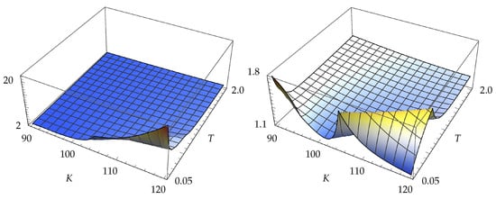
Figure 3. On the left, there is the ratio $\mathbb{V}\left[{\Delta }_{\sigma }^{\mathrm{LR}}\left(c\right)\right]/\mathbb{V}\left[{\Delta }_{\sigma }^{\mathrm{AMVD}}\left(c\right)\right]$ and, on the right, there is the ratio $\mathbb{V}\left[{\Delta }_{\sigma }^{\mathrm{PW}}\left(c\right)\right]/\mathbb{V}\left[{\Delta }_{\sigma }^{\mathrm{AMVD}}\left(c\right)\right]$.

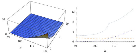
Figure 4. On the left, there is the ratio $\mathbb{V}\left[{\Delta }_{\sigma }^{\mathrm{PW}}\left(c\right)\right]/\mathbb{V}\left[{\Delta }_{\sigma }^{\mathrm{AMVD}}\left(c\right)\right]$. On the right, there are variance ratios at $T=0.1$. The solid curve is $\mathbb{V}\left[{\Delta }_{\sigma }^{\mathrm{LR}}\left(c\right)\right]/\mathbb{V}\left[{\Delta }_{\sigma }^{\mathrm{AMVD}}\left(c\right)\right]$, the dashed curve is $\mathbb{V}\left[{\Delta }_{\sigma }^{\mathrm{MVD}}\left(c\right)\right]/\mathbb{V}\left[{\Delta }_{\sigma }^{\mathrm{AMVD}}\left(c\right)\right]$, and the dotted curve is $\mathbb{V}\left[{\Delta }_{\sigma }^{\mathrm{PW}}\left(c\right)\right]/\mathbb{V}\left[{\Delta }_{\sigma }^{\mathrm{AMVD}}\left(c\right)\right]$.

6. Digital Calls

In this section, we compute the LR, MVD, and AMVD variances for the digital call deltas and vegas. Once again, we only provide details for digital calls; let K be the strike for a digital call with expiry T.

6.1. Digital Call Delta

The likelihood ratio delta for the digital call is computed using the expression

$$\begin{array}{c}\hfill \mathbb{E}\left[{\Delta }_{S_0}^{\mathrm{LR}}\left(d\right)\right]={\int }_{-{\xi }_{-}}^{\infty }\frac{e^{-rT}\xi }{S_0\varsigma }\varphi \left(\xi \right)d\xi =\frac{e^{-rT}}{S_0\varsigma }\varphi \left({\xi }_{-}\right),\end{array}$$

and the associated variance is

$$\begin{array}{c}\hfill \mathbb{V}\left[{\Delta }_{S_0}^{\mathrm{LR}}\left(d\right)\right]=\frac{e^{-2rT}}{S_0^2{\varsigma }^2}\left[\mathcal{I}\left(x^2,0;-{\xi }_{-},\infty \right)-{\varphi }^2\left({\xi }_{-}\right)\right].\end{array}$$

(53)

The MVD delta for the digital call is computed using the expression

$$\begin{array}{c}\hfill \mathbb{E}\left[{\Delta }_{S_0}^{\mathrm{MVD}}\left(d\right)\right]={\int }_{0\vee -{\xi }_{-}}^{\infty }\frac{e^{-rT}}{S_0\varsigma \sqrt{2\pi }}\sqrt{2\pi }\xi \varphi \left(\xi \right)d\xi -{\int }_{0\wedge -{\xi }_{-}}^0\frac{e^{-rT}}{S_0\varsigma \sqrt{2\pi }}\sqrt{2\pi }(-\xi )\varphi \left(\xi \right)d\xi ,\end{array}$$

and the variance is given by

$$\begin{array}{c}\hfill \begin{array}{cc}\hfill \mathbb{V}\left[{\Delta }_{S_0}^{\mathrm{MVD}}\left(d\right)\right]=\frac{e^{-2rT}}{S_0^2{\varsigma }^2\sqrt{2\pi }}& \left[\mathcal{I}\left(x,0;0\vee -{\xi }_{-},\infty \right)-\mathcal{I}\left(x,0;0\wedge -{\xi }_{-},0\right)\right.\hfill \\ & \left.-\sqrt{2\pi }{\varphi }^2\left({\xi }_{-}\right)\right].\hfill \end{array}\end{array}$$

(54)

Finally, AMVD delta for the digital is given by

$$\begin{array}{c}\hfill \mathbb{E}\left[{\Delta }_{S_0}^{\mathrm{AMVD}}\left(d\right)\right]={\int }_{-{\xi }_{-}}^{\infty }\frac{e^{-rT}}{S_0\varsigma }\sqrt{\frac{2}{\pi }}·\sqrt{\frac{\pi }{2}}\left|\xi \right|\varphi \left(\xi \right)d\xi ,\end{array}$$

with the associated variance

$$\begin{array}{c}\hfill \begin{array}{cc}\hfill \mathbb{V}\left[{\Delta }_{S_0}^{\mathrm{AMVD}}\left(d\right)\right]=\frac{e^{-2rT}}{S_0^2{\varsigma }^2}\sqrt{\frac{2}{\pi }}& \left[\mathcal{I}\left(x,0;0\vee -{\xi }_{-},\infty \right)-\mathcal{I}\left(x,0;0\wedge -{\xi }_{-},0\right)-\sqrt{\frac{\pi }{2}}{\varphi }^2\left({\xi }_{-}\right)\right].\hfill \end{array}\end{array}$$

We note that the PW method cannot be applied for digital options.

The ratios of variances for digital call delta are shown in Figure 5. The AMVD method gives lower variances than the LR method, particularly for short-dated deep in-the-money digitals. The MVD method gives lower variances than the AMVD method, most noticeably for at-the-money digitals.

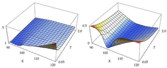
Figure 5. On the left, there is the ratio $\mathbb{V}\left[{\Delta }_{S_0}^{\mathrm{LR}}\left(d\right)\right]/\mathbb{V}\left[{\Delta }_{S_0}^{\mathrm{AMVD}}\left(d\right)\right]$ and, on the right, there is the ratio $\mathbb{V}\left[{\Delta }_{S_0}^{\mathrm{MVD}}\left(d\right)\right]/\mathbb{V}\left[{\Delta }_{S_0}^{\mathrm{AMVD}}\left(d\right)\right]$.

6.2. Digital Call Vega

The likelihood ratio vega for the digital call is computed using the expression

$$\begin{array}{c}\hfill \mathbb{E}\left[{\Delta }_{\sigma }^{\mathrm{LR}}\left(d\right)\right]={\int }_{-{\xi }_{-}}^{\infty }\frac{e^{-rT}}{\sigma }{q}_{\varsigma }\left(\xi \right)·\varphi \left(\xi \right)d\xi =\frac{e^{-rT}{\xi }_{+}}{\sigma }\varphi \left({\xi }_{-}\right),\end{array}$$

and the associated variance is

$$\begin{array}{cc}\hfill \mathbb{V}\left[{\Delta }_{\sigma }^{\mathrm{LR}}\left(d\right)\right]& =\frac{e^{-2rT}}{{\sigma }^2}\left[\mathcal{I}\left(q_{\varsigma }^2\left(x\right),0;-{\xi }_{-},\infty \right)-{\xi }_{+}^2{\varphi }^2\left({\xi }_{-}\right)\right].\hfill \end{array}$$

(55)

The MVD vega for the digital call is computed using the expression

$$\begin{array}{cc}\hfill \mathbb{E}\left[{\Delta }_{\sigma }^{\mathrm{MVD}}\left(d\right)\right]& ={\int }_{-{\xi }_{-}}^{\infty }\frac{e^{-rT}}{\sigma }·{\xi }^2\varphi \left(\xi \right)d\xi -{\int }_{0\vee -{\xi }_{-}}^{\infty }\frac{e^{-rT}}{\sigma \sqrt{2\pi }}·\sqrt{2\pi }\xi \varphi \left(\xi \right)d\xi \hfill \\ & +{\int }_{0\wedge -{\xi }_{-}}^0\frac{e^{-rT}}{\sigma \sqrt{2\pi }}·\sqrt{2\pi }(-\xi )\varphi \left(\xi \right)d\xi -{\int }_{-{\xi }_{-}}^{\infty }\frac{e^{-rT}}{\sigma }·\varphi \left(\xi \right)d\xi ,\hfill \end{array}$$

and the associated variance is given by

$$\begin{array}{c}\hfill \begin{array}{cc}\hfill \mathbb{V}\left[{\Delta }_{\sigma }^{\mathrm{MVD}}\left(d\right)\right]& =\frac{e^{-2rT}}{{\sigma }^2}\left[\mathcal{I}\left(x^2,0;-{\xi }_{-},\infty \right)+\mathcal{I}\left(1,0;-{\xi }_{-},\infty \right)-{\xi }_{+}^2{\varphi }^2\left({\xi }_{-}\right)\right]\hfill \\ & +\frac{e^{-2rT}}{{\sigma }^2\sqrt{2\pi }}\left[\mathcal{I}\left(x,0;0\vee -{\xi }_{-},\infty \right)-\mathcal{I}\left(x,0;0\wedge -{\xi }_{-},0\right)\right].\hfill \end{array}\end{array}$$

(56)

Finally, the AMVD vega for the digital call is computed using the expression

$$\begin{array}{cc}\hfill \mathbb{E}\left[{\Delta }_{\sigma }^{\mathrm{AMVD}}\left(d\right)\right]& ={\int }_{-{\xi }_{-}}^{\infty }\frac{e^{-rT}{\eta }_{\varsigma }}{\sigma }·\frac{1}{{\eta }_{\varsigma }}\left|q_{\varsigma }\left(\xi \right)\right|\varphi \left(\xi \right)d\xi ,\hfill \end{array}$$

with the associated variance

$$\begin{array}{c}\hfill \begin{array}{cc}\hfill \mathbb{V}\left[{\Delta }_{\sigma }^{\mathrm{AMVD}}\left(d\right)\right]=\frac{e^{-2rT}{\eta }_{\varsigma }}{{\sigma }^2}& \left[\mathcal{I}\left(q\left(x\right),0;{\varsigma }_{+}\vee -{\xi }_{-},\infty \right)\phantom{\frac{{\xi }_{+}^2}{{\eta }_{\varsigma }}}\right.\hfill \\ & -\mathcal{I}\left(q\left(x\right),0;\left({\varsigma }_{-}\vee -{\xi }_{-}\right)\wedge {\varsigma }_{+},{\varsigma }_{+}\right)\hfill \\ & \left.+\mathcal{I}\left(q\left(x\right),0;{\varsigma }_{-}\wedge -{\xi }_{-},{\varsigma }_{-}\right)-\frac{{\xi }_{+}^2}{{\eta }_{\varsigma }}{\varphi }^2\left({\xi }_{-}\right)\right].\hfill \end{array}\end{array}$$

(57)

The ratios of variances for digital calls are shown in Figure 6, where it can be seen that the AMVD method gives lower variance than both the LR and the MVD methods.

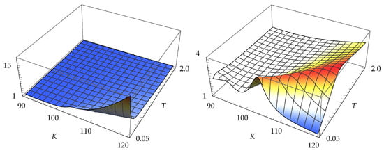
Figure 6. On the left, there is the ratio $\mathbb{V}\left[{\Delta }_{\sigma }^{\mathrm{LR}}\left(d\right)\right]/\mathbb{V}\left[{\Delta }_{\sigma }^{\mathrm{AMVD}}\left(d\right)\right]$ and, on the right, there is the ratio $\mathbb{V}\left[{\Delta }_{\sigma }^{\mathrm{MVD}}\left(d\right)\right]/\mathbb{V}\left[{\Delta }_{\sigma }^{\mathrm{AMVD}}\left(d\right)\right]$.

7. Double-Barrier Option

In this section, we consider the delta and vega for a double-barrier option that knocks out if the closing price of the underlying asset lies outside the range, $]B_L,B_U[$, on at least three days prior to expiry, where $B_L<B_U$, and pays the constant rebate $R=100$ otherwise. We take $S_0=100$, $T=0.25$, $\sigma =0.20$, and subdivide the interval $[0,25]$ into 90 equal subintervals. This is the example considered in Chan and Joshi (2015) Subsection 5.3.

7.1. Generation of Non-Normal Random Variates

In order to implement the AMVD method, and the MVD method for comparison purposes, we need to generate random variates from the Rayleigh distribution, the double-sided Maxwell–Boltzmann distribution, and the distributions corresponding to the absolute value densities appearing in (23) and (24).

7.1.1. Rayleigh Random Variate

The standard Rayleigh distribution is defined for $x\ge 0$ and has the probability density function

$$\begin{array}{cc}\hfill {\varphi }_{\mathrm{R}}\left(x\right)& =x{e}^{-\frac{1}{2}{x}^2},\hfill \end{array}$$

(58)

and the cumulative density function

$$\begin{array}{cc}\hfill {\Phi }_{\mathrm{R}}\left(x\right)& =1-e^{-\frac{1}{2}{x}^2}.\hfill \end{array}$$

(59)

Since the inverse of the cumulative density function is given by

$$\begin{array}{cc}\hfill {\Phi }_{\mathrm{R}}^{-1}\left(x\right)& =\sqrt{-2ln(1-x)}\hfill \end{array}$$

(60)

for $x\in [0,1[$, a variate from the Rayleigh distribution can be generated using the following algorithm:

R1.

Generate a uniform variate $u\in [0,1[$.

R2.

Set $x={\Phi }_{\mathrm{R}}^{-1}\left(u\right)=\sqrt{-2ln(1-u)}$, which is then a Rayleigh random variate.

7.1.2. Double-Sided Maxwell–Boltzmann Random Variate

The standard Maxwell–Boltzmann distribution is defined for $x\ge 0$ and has probability density function

$$\begin{array}{c}\hfill {\varphi }_{\mathrm{MB}}\left(x\right)=\sqrt{\frac{2}{\pi }}{x}^2{e}^{-\frac{1}{2}{x}^2}.\end{array}$$

(61)

An algorithm for generating variates from the Maxwell–Boltzmann distribution based on the acceptance–rejection method, and introduced in Heidergott et al. (2008), is as follows:

MB1.

Generate independent uniform variates $u_1,u_2\in [0,1$[. Set $w=\sqrt{-4ln\left(u_1\right)}$.

MB2.

If $u_2>1.16582199u_{1}w$, then go back to step MB1.3

MB3.

Generate a uniform variate $u_3\in [0,1[$, independent of $u_1$ and $u_2$.

MB4.

If $u_3<0.5$, set $x=w$, and set $x=-w$ otherwise. Then, x is a double-sided Maxwell–Boltzmann random variate.

7.1.3. Absolute Rayleigh Distribution

Consider the random variable with domain $\mathbb{R}$, and the probability density function

$$\begin{array}{c}\hfill {\varphi }_{\left|\mathrm{R}\right|}\left(x\right)=\frac{1}{2}\left|x\right|e^{-\frac{1}{2}{x}^2}.\end{array}$$

(62)

Note that ${\varphi }_{\left|\mathrm{R}\right|}$ is obtained by extending ${\varphi }_{\mathrm{R}}$ to $\mathbb{R}$ using symmetry about the vertical axis. Hence, an algorithm for generating a variate from the absolute Rayleigh distribution is as follows:

AR1.

Generate a uniform variate $u\in ]0,1[$.

AR2.

Then, an absolute Rayleigh random variate, x, is given by

$$\begin{array}{c}\hfill x=\left\{\begin{array}{cc}\sqrt{-2ln\left(2\right(1-u\left)\right)},\hfill & \mathrm{if}u\ge \frac{1}{2},\hfill \\ -\sqrt{-2ln\left(2u\right)},\hfill & \mathrm{if}u<\frac{1}{2}.\hfill \end{array}\right.\end{array}$$

(63)

7.1.4. Absolute Quadratic Normal (AQN) Distribution

Assume $\varsigma \in {\mathbb{R}}_{+}$, and let $q_{\varsigma }$, ${\eta }_{\varsigma }$, and ${\varsigma }_{\pm }$ be as defined in (29), (49), and (50), respectively. Consider the random variable with domain $\mathbb{R}$, and the probability density function

$$\begin{array}{c}\hfill {\varphi }_{\mathrm{AQN}}(x;\varsigma )=\frac{1}{{\eta }_{\varsigma }}\left|q_{\varsigma }\left(x\right)\right|\varphi \left(x\right).\end{array}$$

(64)

Note that ${\varsigma }_{\pm }$ are the roots of $q_{\varsigma }\left(x\right)$, and  $q_{\varsigma }\left(x\right)<0$ for $x\in \left]{\varsigma }_{-},{\varsigma }_{+}\right[$. If we denote by ${\Phi }_{\mathrm{AQN}}$ the corresponding cumulative density function, then a straight forward calculation gives

$$\begin{array}{c}\hfill {\Phi }_{\mathrm{AQN}}(x;\varsigma )=\frac{1}{{\eta }_{\varsigma }}\left\{\begin{array}{cc}\left(\varsigma -x\right)\varphi \left(x\right),\hfill & x\le {\varsigma }_{-},\hfill \\ 2\left(\varsigma -{\varsigma }_{-}\right)\varphi \left({\varsigma }_{-}\right)+\left(x-\varsigma \right)\varphi \left(x\right),\hfill & {\varsigma }_{-}<x\le {\varsigma }_{+},\hfill \\ {\eta }_{\varsigma }-\left(x-\varsigma \right)\varphi \left(x\right),\hfill & x>{\varsigma }_{+}.\hfill \end{array}\right.\end{array}$$

(65)

Note that, in each of the three regions, ${\Phi }_{\mathrm{AQN}}(x;\varsigma )$ has the form

$$\begin{array}{c}\hfill \frac{1}{{\eta }_{\varsigma }}\left[\alpha +ϵ(x-\varsigma )\varphi \left(x\right)\right],\end{array}$$

where $\alpha \in \mathbb{R}$ and $ϵ=\pm 1$. Thus, given a uniform random variate u, to compute the corresponding variate with density ${\varphi }_{\mathrm{AQN}}(x;\varsigma )$, we need to compute the root of a function of the form

$$\begin{array}{c}\hfill h\left(x\right)=\frac{1}{{\eta }_{\varsigma }}\left[\alpha +ϵ(x-\varsigma )\varphi \left(x\right)\right]-u,\end{array}$$

with $\alpha$ and $ϵ$ appropriately chosen according to the value of u. For this purpose, we apply Newton’s method noting that

$$\begin{array}{c}\hfill h^{\prime }\left(x\right)=-\frac{ϵ}{{\eta }_{\varsigma }}\left(x^2-\varsigma x-1\right)\varphi \left(x\right)=-\frac{ϵ}{{\eta }_{\varsigma }}{q}_{\varsigma }\left(x\right)\varphi \left(x\right).\end{array}$$

Thus, given an initial point $x^{\left(0\right)}$, we can apply the recursion

$$\begin{array}{c}\hfill x^{(i+1)}=x^{\left(i\right)}-\frac{h\left(x^{\left(i\right)}\right)}{h^{\prime }\left(x^{\left(i\right)}\right)},\end{array}$$

(66)

until the desired degree of precision is achieved.

However, due to the nature of $h\left(x\right)$, Newton’s method can be highly sensitive to the initial point $x^{\left(0\right)}$. In fact, a poor initial value can result in the method failing to converge to the correct root. Thus, it is crucial that the initial point is chosen carefully, and, for this, we take inspiration from Heidergott et al. (2008) where the Weibull distribution is used in the acceptance–rejection method to generate the double-sided Maxwell–Boltzmann distribution.

For the two regions, $]-\infty ,{\varsigma }_{-}]$ and $]{\varsigma }_{+},\infty [$, we approximate the AQN density using Weibull distributions

$$\begin{array}{c}\hfill {\varphi }_{\mathrm{W}}^{\pm }\left(x\right)=\mp 2{\beta }_{\pm }\left(x-{\varsigma }_{\pm }\right)e^{-{\beta }_{\pm }{\left(x-{\varsigma }_{\pm }\right)}^2},\end{array}$$

(67)

with the cumulative density function

$$\begin{array}{c}\hfill {\Phi }_W^{\pm }\left(x\right)=e^{-{\beta }_{\pm }{\left(x-{\varsigma }_{\pm }\right)}^2}.\end{array}$$

(68)

The parameters, ${\beta }_{\pm }$, are determined by matching the variances of the approximating Weibull distributions to the variances of the AQN variate restricted to the intervals ]$-\infty ,{\varsigma }_{-}]$ and ]${\varsigma }_{+},\infty [$, respectively. This gives

$$\begin{array}{c}\hfill {\beta }_{\pm }=\frac{1}{{\sigma }_{\pm }^2}\left(1-\frac{\pi }{4}\right).\end{array}$$

(69)

where ${\sigma }_{\pm }^2$ are variances of the AQN variate restricted to ]$-\infty ,{\varsigma }_{-}]$ and $]{\varsigma }_{+},\infty$[. For the details, refer to Appendix A.

For the region $[{\varsigma }_{-},{\varsigma }_{+}]$, we approximate the AQN cumulative density on $[{\varsigma }_{-},{\varsigma }_m]$ and $[{\varsigma }_m,{\varsigma }_{+}]$, where ${\varsigma }_m=\frac{1}{2}\left({\varsigma }_{-}+{\varsigma }_{+}\right)$, using quadratics

$$\begin{array}{cc}\hfill q_{-}\left(x\right)& =c_{-}{\left(x-{\varsigma }_{-}\right)}^2,\mathrm{and}\hfill \\ \hfill q_{+}\left(x\right)& ={\Phi }_{\mathrm{AQN}}\left({\varsigma }_{+};\varsigma \right)-{\Phi }_{\mathrm{AQN}}\left({\varsigma }_{-};\varsigma \right)-c_{+}{\left(x-{\varsigma }_{+}\right)}^2,\hfill \end{array}$$

with $c_{\pm }$ determined by setting $q_{-}\left({\varsigma }_m\right)={\Phi }_{\mathrm{AQN}}\left({\varsigma }_m;\varsigma \right)-{\Phi }_{\mathrm{AQN}}\left({\varsigma }_{-};\varsigma \right)=q_{+}\left({\varsigma }_m\right)$, which gives   

$$\begin{array}{cc}\hfill c_{-}& =\frac{{\Phi }_{\mathrm{AQN}}({\varsigma }_m;\varsigma )-{\Phi }_{\mathrm{AQN}}\left({\varsigma }_{-};\varsigma \right)}{{\left({\varsigma }_m-{\varsigma }_{-}\right)}^2},\hfill \end{array}$$

(70)

$$\begin{array}{cc}\hfill c_{+}& =\frac{{\Phi }_{\mathrm{AQN}}({\varsigma }_{+};\varsigma )-{\Phi }_{\mathrm{AQN}}\left({\varsigma }_m;\varsigma \right)}{{\left({\varsigma }_m-{\varsigma }_{+}\right)}^2}.\hfill \end{array}$$

(71)

The objective function, h, and the initial point, $x^{\left(0\right)}$, for the four regions determined by the uniform random variate $u\in ]0,1[$ are shown in Table 1.

Table 1. Objective functions and the initial values for generating the AQN random variate using Newton’s method, where $u_{\pm }={\Phi }_{\mathrm{AQN}}({\varsigma }_{\pm };\varsigma )$.

u	$\mathit{h}\left(\mathit{x}\right)+\mathit{u}$	${\mathit{x}}^{\left(0\right)}$
]$0,u_{-}]$	${\displaystyle \frac{1}{{\eta }_{\varsigma }}}(\varsigma -x)\varphi \left(x\right)$	${\varsigma }_{-}-\sqrt{-{\displaystyle \frac{1}{{\beta }_{-}}}ln\left({\displaystyle \frac{u}{u_{-}}}\right)}$
$\left]u_{-},\frac{1}{2}(u_{-}+u_{+})\right]$	${\displaystyle \frac{2}{{\eta }_{\varsigma }}}(\varsigma -{\varsigma }_{-})\varphi \left({\varsigma }_{-}\right)+{\displaystyle \frac{1}{{\eta }_{\varsigma }}}(x-\varsigma )\varphi \left(x\right)$	${\varsigma }_{-}+\sqrt{{\displaystyle \frac{u-u_{-}}{c_{-}}}}$
$\left]\frac{1}{2}(u_{-}+u_{+}),u_{+}\right]$	${\displaystyle \frac{2}{{\eta }_{\varsigma }}}(\varsigma -{\varsigma }_{-})\varphi \left({\varsigma }_{-}\right)+{\displaystyle \frac{1}{{\eta }_{\varsigma }}}(x-\varsigma )\varphi \left(x\right)$	${\varsigma }_{+}-\sqrt{{\displaystyle \frac{u_{+}-u}{c_{+}}}}$
$\left]u_{+},1\right[$	$1-{\displaystyle \frac{1}{{\eta }_{\varsigma }}}(x-\varsigma )\varphi \left(x\right)$	${\varsigma }_{+}+\sqrt{-{\displaystyle \frac{1}{{\beta }_{+}}}ln\left({\displaystyle \frac{1-u}{1-u_{+}}}\right)}$

Using the initial values given in Table 1, Newton’s method converges within four iterations in most cases. It should be noted that each Newton iteration only involves elementary operations and one exponential, and so the method is quite computationally efficient.

7.2. Double-Barrier Vega

Vegas for the double knock-out barrier was computed using a Monte Carlo simulation implemented in C++ with uniform random variates generated by Mersenne Twister from the boost library.4 For each method, 100 independent valuations were performed with each valuation using 50,000 paths for the MVD method and 100,000 paths for the LR and AMVD methods. Standard deviations were then computed from these 100 samples. The lower and upper barriers were set to $L_i=75+2i$ and $U_i=105+2j$ for $0\le i,j\le 10$. The resulting means and standard deviations of vegas for a subset of $(L_i,U_i)$ pairs is shown in Table 2.

Table 2. Means and standard deviations of vegas for double-barrier options with varying lower and upper barriers using the LR, MVD, and AMVD methods.

		Mean			Standard Deviation
$\mathit{L}$	$\mathit{U}$	LR	MVD	AMVD	LR	MVD	AMVD
75	105	−169.34	−167.52	−168.29	15.68	7.69	11.17
75	115	−173.85	−172.96	−171.81	19.51	6.43	13.65
75	125	−60.85	−60.17	−60.39	20.08	3.25	15.7
85	105	−292.55	−291.65	−292.08	12.04	8.6	10.75
85	115	−305.83	−306.81	−307.69	19.13	8.05	14.14
85	125	−193.72	−195.74	−195.11	21.13	6.26	13.96
95	105	−146.66	−147.24	−146.53	5.67	7.77	5.92
95	115	−316.54	−317.12	−318.45	13.47	10.15	10.38
95	125	−220.83	−219.58	−218.19	14.36	7.8	10.75

It is evident from Figure 7 that MVD vegas have the lowest standard deviations in general for double-barrier options, followed by those of the AMVD, and then the LR method. It is worth noting that the standard deviation in vegas for the AMVD method is lowest, in relative terms, when the upper barrier is close to the lower barrier. In fact, the AMVD method has the lowest standard deviation among the three methods when $(L,U)=(95,105)$.

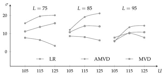
Figure 7. Comparison of double-barrier option vega standard deviations for the LR, MVD, and AMVD methods.

This is consistent with an observation made in previous sections that the method giving sensitivities with the smallest variance will not only depend on the derivative being considered but also on the details such as strikes and barrier levels, and the way each method distributes densities relative to the strikes and barriers. The implementer should experiment and choose the method that is most appropriate for each application.

8. Conclusions

In this paper, we introduced an alternative to the measure-valued differentiation (MVD) method for computing Monte Carlo sensitivities, called the absolute measure-valued differentiation (AMVD) method, which decomposes the density derivative as the product of its sign and its absolute value. This method shares many of the properties of the MVD method, but instead of initiating two additional paths in each simulation step of the original path, it initiates only one additional subpath. It was shown that the AMVD method gives vega estimates with lower variance than the MVD method for vanilla and digital calls in the Black–Scholes model. Moreover, the AMVD vega estimates have lower variance than the pathwise differentiation method in certain situations, such as the case of short-dated deep in-the-money vanilla calls. A consideration of the vegas for the more exotic double-barrier options revealed that the relative performances of the likelihood ratio, MVD, and AMVD methods depend, in general, on the positions of the barriers, and the way each method distributes densities relative to the barriers.

As is the case with the MVD method, applying the AMVD method requires the generation of nonstandard random variates. For the examples considered in this paper, we provided a highly efficient implementation of the inverse transform method for this purpose using Newton’s method with a careful selection of the initial point.

Appendix B.1. Likelihood Ratio Call Delta Variance

The second moment associated with the likelihood ratio delta for the vanilla call is given by

$$\begin{array}{cc}\hfill & m^{\left(2\right)}\left[{\Delta }_{S_0}^{\mathrm{LR}}\right]={\int }_{-{\xi }_{-}}^{\infty }{\left[e^{-rT}\left(S_0{e}^{\left(r-\frac{1}{2}{\sigma }^2\right)T+\varsigma \xi }-K\right)\frac{\xi }{S_0\varsigma }\right]}^2\varphi \left(\xi \right)d\xi \hfill \\ \hfill & =\frac{e^{-2rT}}{S_0^2{\varsigma }^2}{\int }_{-{\xi }_{-}}^{\infty }\left[S_0^2{e}^{\left(2r-{\sigma }^2\right)T+2\varsigma \xi }-2K{S}_0{e}^{\left(r-\frac{1}{2}{\sigma }^2\right)T+\varsigma \xi }+K^2\right]{\xi }^2\varphi \left(\xi \right)d\xi .\hfill \end{array}$$

Computing the three terms, we obtain

$$\begin{array}{cc}\hfill m_{S_0,1}^{\mathrm{LR}}& =\frac{e^{-{\varsigma }^2}}{{\varsigma }^2}{\int }_{-{\xi }_{-}}^{\infty }{e}^{2\varsigma \xi }{\xi }^2\varphi \left(\xi \right)d\xi =\frac{e^{{\varsigma }^2}}{{\varsigma }^2}\mathcal{I}\left(x^2,2\varsigma ;-{\xi }_{-},\infty \right),\hfill \\ \hfill m_{S_0,2}^{\mathrm{LR}}& =-\frac{2K{e}^{-\left(r+\frac{1}{2}{\sigma }^2\right)T}}{S_0{\varsigma }^2}{\int }_{-{\xi }_{-}}^{\infty }{e}^{\varsigma \xi }{\xi }^2\varphi \left(\xi \right)d\xi =-\frac{2K{e}^{-rT}}{S_0{\varsigma }^2}\mathcal{I}\left(x^2,\varsigma ;-{\xi }_{-},\infty \right),\hfill \\ \hfill m_{S_0,3}^{\mathrm{LR}}& =\frac{K^2{e}^{-2rT}}{S_0^2{\varsigma }^2}{\int }_{-{\xi }_{-}}^{\infty }{\xi }^2\varphi \left(\xi \right)d\xi =\frac{K^2{e}^{-2rT}}{S_0^2{\varsigma }^2}\mathcal{I}\left(x^2,0;-{\xi }_{-},\infty \right).\hfill \end{array}$$

Appendix B.2. MVD Call Delta Variance

The second moment for the MVD delta estimate is given by

$$\begin{array}{cc}\hfill m^{\left(2\right)}\left[{\Delta }_{S_0}^{\mathrm{MVD}}\right]& ={\int }_{0\vee -{\xi }_{-}}^{\infty }{\left[\frac{e^{-rT}}{S_0\varsigma \sqrt{2\pi }}\left(S_0{e}^{\left(r-\frac{1}{2}{\sigma }^2\right)T+\varsigma \xi }-K\right)\right]}^2·\sqrt{2\pi }\xi \varphi \left(\xi \right)d\xi \hfill \\ & +{\int }_{0\wedge -{\xi }_{-}}^0{\left[\frac{e^{-rT}}{S_0\varsigma \sqrt{2\pi }}\left(S_0{e}^{\left(r-\frac{1}{2}{\sigma }^2\right)T+\varsigma \xi }-K\right)\right]}^2·\sqrt{2\pi }(-\xi )\varphi \left(\xi \right)d\xi .\hfill \end{array}$$

Computing the first term, we obtain

$$\begin{array}{c}\hfill \frac{e^{-2rT}}{\sqrt{2\pi }{S}_0^2{\varsigma }^2}{\int }_{0\vee -{\xi }_{-}}^{\infty }\left[S_0^2{e}^{\left(2r-{\sigma }^2\right)T+2\varsigma \xi }-2K{S}_0{e}^{\left(r-\frac{1}{2}{\sigma }^2\right)T+\varsigma \xi }+K^2\right]\xi \varphi \left(\xi \right)d\xi ,\end{array}$$

and the three subterms are given by

$$\begin{array}{cc}\hfill m_{S_0,1,1}^{\mathrm{MVD}}& =\frac{e^{-{\varsigma }^2}}{\sqrt{2\pi }{\varsigma }^2}{\int }_{0\vee -{\xi }_{-}}^{\infty }{e}^{2\varsigma \xi }\xi \varphi \left(\xi \right)d\xi =\frac{e^{{\varsigma }^2}}{\sqrt{2\pi }{\varsigma }^2}\mathcal{I}\left(x,2\varsigma ;0\vee -{\xi }_{-},\infty \right),\hfill \\ \hfill m_{S_0,1,2}^{\mathrm{MVD}}& =-\frac{2K{e}^{-\left(r+\frac{1}{2}{\sigma }^2\right)T}}{\sqrt{2\pi }{S}_0{\varsigma }^2}{\int }_{0\vee -{\xi }_{-}}^{\infty }{e}^{\varsigma \xi }\xi \varphi \left(\xi \right)d\xi =-\frac{2K{e}^{-rT}}{\sqrt{2\pi }{S}_0{\varsigma }^2}\mathcal{I}\left(x,\varsigma ;0\vee -{\xi }_{-},\infty \right),\hfill \\ \hfill m_{S_0,1,3}^{\mathrm{MVD}}& =\frac{K^2{e}^{-2rT}}{\sqrt{2\pi }{S}_0^2{\varsigma }^2}{\int }_{0\vee -{\xi }_{-}}^{\infty }\xi \varphi \left(\xi \right)d\xi =\frac{K^2{e}^{-2rT}}{\sqrt{2\pi }{S}_0^2{\varsigma }^2}\mathcal{I}\left(x,0;0\vee -{\xi }_{-},\infty \right).\hfill \end{array}$$

Similarly, computing the second term, we obtain

$$\begin{array}{c}\hfill \frac{e^{-2rT}}{\sqrt{2\pi }{S}_0^2{\varsigma }^2}{\int }_{0\wedge -{\xi }_{-}}^0\left[S_0^2{e}^{\left(2r-{\sigma }^2\right)T+2\varsigma \xi }-2K{S}_0{e}^{\left(r-\frac{1}{2}{\sigma }^2\right)T+\varsigma \xi }+K^2\right](-\xi )\varphi \left(\xi \right)d\xi ,\end{array}$$

and the three subterms are given by

$$\begin{array}{cc}\hfill m_{S_0,2,1}^{\mathrm{MVD}}& =-\frac{e^{-{\varsigma }^2}}{\sqrt{2\pi }{\varsigma }^2}{\int }_{0\wedge -{\xi }_{-}}^0{e}^{2\varsigma \xi }\xi \varphi \left(\xi \right)d\xi =-\frac{e^{{\varsigma }^2}}{\sqrt{2\pi }{\varsigma }^2}\mathcal{I}\left(x,2\varsigma ;0\wedge -{\xi }_{-},0\right),\hfill \\ \hfill m_{S_0,2,2}^{\mathrm{MVD}}& =\frac{2K{e}^{-\left(r+\frac{1}{2}{\sigma }^2\right)T}}{\sqrt{2\pi }{S}_0{\varsigma }^2}{\int }_{0\wedge -{\xi }_{-}}^0{e}^{\varsigma \xi }\xi \varphi \left(\xi \right)d\xi =\frac{2K{e}^{-rT}}{\sqrt{2\pi }{S}_0{\varsigma }^2}\mathcal{I}\left(x,\varsigma ;0\wedge -{\xi }_{-},0\right),\hfill \\ \hfill m_{S_0,2,3}^{\mathrm{MVD}}& =-\frac{K^2{e}^{-2rT}}{\sqrt{2\pi }{S}_0^2{\varsigma }^2}{\int }_{0\wedge -{\xi }_{-}}^0\xi \varphi \left(\xi \right)d\xi =\frac{K^2{e}^{-2rT}}{\sqrt{2\pi }{S}_0^2{\varsigma }^2}\mathcal{I}\left(x,0;0\wedge -{\xi }_{-},0\right).\hfill \end{array}$$

Appendix B.3. AMVD Call Delta Variance

The second moment for the AMVD delta estimate is given by

$$\begin{array}{cc}\hfill m^{\left(2\right)}\left[{\Delta }_{S_0}^{\mathrm{AMVD}}\right]& =2{\int }_{-{\xi }_{-}}^{\infty }{\left[\frac{e^{-rT}}{S_0\varsigma \sqrt{2\pi }}\left(S_0{e}^{\left(r-\frac{1}{2}{\sigma }^2\right)T+\varsigma \xi }-K\right)\right]}^2·\sqrt{2\pi }\left|\xi \right|\varphi \left(\xi \right)d\xi \hfill \\ & =2m^{\left(2\right)}\left[{\Delta }_{S_0}^{\mathrm{MVD}}\right].\hfill \end{array}$$

Appendix B.4. Likelihood Ratio Call Vega Variance

The second moment associated with the likelihood ratio vega for the vanilla call is given by

$$\begin{array}{c}\hfill m^{\left(2\right)}\left[{\Delta }_{\sigma }^{\mathrm{LR}}\right]=\frac{e^{-2rT}}{{\sigma }^2}{\int }_{-{\xi }_{-}}^{\infty }{\left[S_0{e}^{\left(r-\frac{1}{2}{\sigma }^2\right)T+\sigma \sqrt{T}\xi }-K\right]}^2{q}^2\left(\xi \right)\varphi \left(\xi \right)d\xi ,\end{array}$$

where $q\left(x\right)$ is as defined in (30). Expanding out the first term, we obtain

$$\begin{array}{c}\hfill m^{\left(2\right)}\left[{\Delta }_{\sigma }^{\mathrm{LR}}\right]=\frac{e^{-2rT}}{{\sigma }^2}{\int }_{-{\xi }_{-}}^{\infty }\left[S_0^2{e}^{\left(2r-{\sigma }^2\right)T+2\varsigma \xi }-2K{S}_0{e}^{\left(r-\frac{1}{2}{\sigma }^2\right)T+\varsigma \xi }+K^2\right]q^2\left(\xi \right)\varphi \left(\xi \right)d\xi .\end{array}$$

Computing the three terms gives

$$\begin{array}{cc}\hfill m_{\sigma ,1}^{\mathrm{LR}}& =\frac{e^{-{\varsigma }^2}{S}_0^2}{{\sigma }^2}{\int }_{-{\xi }_{-}}^{\infty }{e}^{2\varsigma \xi }{q}^2\left(\xi \right)\varphi \left(\xi \right)d\xi =\frac{e^{{\varsigma }^2}{S}_0^2}{{\sigma }^2}\mathcal{I}\left(q^2,2\varsigma ;-{\xi }_{-},\infty \right),\hfill \\ \hfill m_{\sigma ,2}^{\mathrm{LR}}& =-\frac{2e^{-\left(r+\frac{1}{2}{\sigma }^2\right)T}K{S}_0}{{\sigma }^2}{\int }_{-{\xi }_{-}}^{\infty }{e}^{\varsigma \xi }{q}^2\left(\xi \right)\varphi \left(\xi \right)d\xi =-\frac{2e^{-rT}K{S}_0}{{\sigma }^2}\mathcal{I}\left(q^2,\varsigma ;-{\xi }_{-},\infty \right),\hfill \\ \hfill m_{\sigma ,3}^{\mathrm{LR}}& =\frac{e^{-2rT}{K}^2}{{\sigma }^2}{\int }_{-{\xi }_{-}}^{\infty }{q}^2\left(\xi \right)\varphi \left(\xi \right)d\xi =\frac{e^{-2rT}{K}^2}{{\sigma }^2}\mathcal{I}\left(q^2,0;-{\xi }_{-},\infty \right).\hfill \end{array}$$

Appendix B.5. MVD Call Vega Variance

The second moment associated with the MVD vega is given by

$$\begin{array}{c}\hfill \begin{array}{cc}\hfill m^{\left(2\right)}\left[{\Delta }_{\sigma }^{\mathrm{MVD}}\right]& =\frac{e^{-2rT}}{{\sigma }^2}{\int }_{-{\xi }_{-}}^{\infty }{\left[S_0{e}^{\left(r-\frac{1}{2}{\sigma }^2\right)T+\varsigma \xi }-K\right]}^2{\xi }^2\varphi \left(\xi \right)d\xi \hfill \\ & +\frac{e^{-2rT}T}{2\pi }{\int }_{0\vee -{\xi }_{-}}^{\infty }{\left[S_0{e}^{\left(r-\frac{1}{2}{\sigma }^2\right)T+\varsigma \xi }-K\right]}^2\sqrt{2\pi }\xi \varphi \left(\xi \right)d\xi \hfill \\ & +\frac{e^{-2rT}T}{2\pi }{\int }_{0\wedge -{\xi }_{-}}^0{\left[S_0{e}^{\left(r-\frac{1}{2}{\sigma }^2\right)T+\varsigma \xi }-K\right]}^2\sqrt{2\pi }(-\xi )\varphi \left(\xi \right)d\xi \hfill \\ & +\frac{e^{-2rT}}{{\sigma }^2}{\int }_{-{\xi }_{-}}^{\infty }{\left[S_0{e}^{\left(r-\frac{1}{2}{\sigma }^2\right)T+\varsigma \xi }-K\right]}^2\varphi \left(\xi \right)d\xi ,\hfill \end{array}\end{array}$$

(A2)

The four terms are as follows:

$$\begin{array}{cc}\hfill m_{\sigma ,1}^{\mathrm{MVD}}& =\frac{e^{{\varsigma }^2}{S}_0^2}{{\sigma }^2}\mathcal{I}\left(x^2,2\varsigma ;-{\xi }_{-},\infty \right)-\frac{2e^{-rT}K{S}_0}{{\sigma }^2}\mathcal{I}\left(x^2,\varsigma ;-{\xi }_{-},\infty \right)\hfill \\ & +\frac{e^{-2rT}{K}^2}{{\sigma }^2}\mathcal{I}\left(x^2,0;-{\xi }_{-},\infty \right),\hfill \\ \hfill m_{\sigma ,2}^{\mathrm{MVD}}& =\frac{e^{{\varsigma }^2}{S}_0^{2}T}{\sqrt{2\pi }}\mathcal{I}\left(x,2\varsigma ;0\vee -{\xi }_{-},\infty \right)-\frac{2e^{-rT}K{S}_{0}T}{\sqrt{2\pi }}\mathcal{I}\left(x,\varsigma ;0\vee -{\xi }_{-},\infty \right)\hfill \\ & +\frac{e^{-2rT}{K}^{2}T}{\sqrt{2\pi }}\mathcal{I}\left(x,0;0\vee -{\xi }_{-},\infty \right),\hfill \\ \hfill m_{\sigma ,3}^{\mathrm{MVD}}& =-\frac{e^{{\varsigma }^2}{S}_0^{2}T}{\sqrt{2\pi }}\mathcal{I}\left(x,2\varsigma ;0\wedge -{\xi }_{-},0\right)+\frac{2e^{-rT}K{S}_{0}T}{\sqrt{2\pi }}\mathcal{I}\left(x,\varsigma ;0\wedge -{\xi }_{-},0\right)\hfill \\ & -\frac{e^{-2rT}{K}^{2}T}{\sqrt{2\pi }}\mathcal{I}\left(x,0;0\wedge -{\xi }_{-},0\right),\hfill \\ \hfill m_{\sigma ,4}^{\mathrm{MVD}}& =\frac{e^{{\varsigma }^2}{S}_0^2}{{\sigma }^2}\mathcal{I}\left(1,2\varsigma ;-{\xi }_{-},\infty \right)-\frac{2e^{-rT}K{S}_0}{{\sigma }^2}\mathcal{I}\left(1,\varsigma ;-{\xi }_{-},\infty \right)\hfill \\ & +\frac{e^{-2rT}{K}^2}{{\sigma }^2}\mathcal{I}\left(1,0;-{\xi }_{-},\infty \right).\hfill \end{array}$$

Appendix B.6. AMVD Call Vega Variance

The second moment associated with the AMVD vega is given by

$$\begin{array}{c}\hfill \begin{array}{cc}\hfill m^{\left(2\right)}\left[{\Delta }_{\sigma }^{\mathrm{AMVD}}\right]& =\frac{e^{-2rT}{\eta }_{\varsigma }}{{\sigma }^2}{\int }_{{\varsigma }_{+}\vee -{\xi }_{-}}^{\infty }{\left[S_0{e}^{\left(r-\frac{1}{2}{\sigma }^2\right)T+\varsigma \xi }-K\right]}^{2}q\left(x\right)\varphi \left(x\right)dx\hfill \\ & -\frac{e^{-2rT}{\eta }_{\varsigma }}{{\sigma }^2}{\int }_{\left({\varsigma }_{-}\vee -{\xi }_{-}\right)\wedge {\varsigma }_{+}}^{{\varsigma }_{+}}{\left[S_0{e}^{\left(r-\frac{1}{2}{\sigma }^2\right)T+\varsigma \xi }-K\right]}^{2}q\left(x\right)\varphi \left(x\right)dx\hfill \\ & +\frac{e^{-2rT}{\eta }_{\varsigma }}{{\sigma }^2}{\int }_{{\varsigma }_{-}\wedge -{\xi }_{-}}^{{\varsigma }_{-}}{\left[S_0{e}^{\left(r-\frac{1}{2}{\sigma }^2\right)T+\varsigma \xi }-K\right]}^{2}q\left(x\right)\varphi \left(x\right)dx.\hfill \end{array}\end{array}$$

(A3)

The three terms are as follows:

$$\begin{array}{cc}\hfill m_{\sigma ,1}^{\mathrm{AMVD}}& =\frac{e^{{\varsigma }^2}{S}_0^2{\eta }_{\varsigma }}{{\sigma }^2}\mathcal{I}\left(q^2\left(x\right),2\varsigma ;{\varsigma }_{+}\vee -{\xi }_{-},\infty \right)-\frac{2e^{-rT}K{S}_0{\eta }_{\varsigma }}{{\sigma }^2}\mathcal{I}\left(q^2\left(x\right),\varsigma ;{\varsigma }_{+}\vee -{\xi }_{-},\infty \right)\hfill \\ & +\frac{e^{-rT}{K}^2{\eta }_{\varsigma }}{{\sigma }^2}\mathcal{I}\left(q^2\left(x\right),0;{\varsigma }_{+}\vee -{\xi }_{-},\infty \right),\hfill \\ \hfill m_{\sigma ,2}^{\mathrm{AMVD}}& =-\frac{e^{{\varsigma }^2}{S}_0^2{\eta }_{\varsigma }}{{\sigma }^2}\mathcal{I}\left(q^2\left(x\right),2\varsigma ;\left({\varsigma }_{-}\vee -{\xi }_{-}\right)\wedge {\varsigma }_{+},{\varsigma }_{+}\right)\hfill \\ & +\frac{2e^{-rT}K{S}_0{\eta }_{\varsigma }}{{\sigma }^2}\mathcal{I}\left(q^2\left(x\right),\varsigma ;\left({\varsigma }_{-}\vee -{\xi }_{-}\right)\wedge {\varsigma }_{+},{\varsigma }_{+}\right)\hfill \\ & -\frac{e^{-rT}{K}^2{\eta }_{\varsigma }}{{\sigma }^2}\mathcal{I}\left(q^2\left(x\right),0;{\varsigma }_{-}\wedge -{\xi }_{-},\infty \right),\hfill \\ \hfill m_{\sigma ,3}^{\mathrm{AMVD}}& =\frac{e^{{\varsigma }^2}{S}_0^2{\eta }_{\varsigma }}{{\sigma }^2}\mathcal{I}\left(q^2\left(x\right),2\varsigma ;{\varsigma }_{-}\wedge -{\xi }_{-},{\varsigma }_{-}\right)-\frac{2e^{-rT}K{S}_0{\eta }_{\varsigma }}{{\sigma }^2}\mathcal{I}\left(q^2\left(x\right),\varsigma ;{\varsigma }_{-}\wedge -{\xi }_{-},{\varsigma }_{-}\right)\hfill \\ & +\frac{e^{-rT}{K}^2{\eta }_{\varsigma }}{{\sigma }^2}\mathcal{I}\left(q^2\left(x\right),0;{\varsigma }_{-}\wedge -{\xi }_{-},{\varsigma }_{-}\right).\hfill \end{array}$$

Appendix C.1. Likelihood Ratio Digital Call Delta Variance

The second moment associated with the likelihood ratio delta for the digital call is

$$\begin{array}{cc}\hfill m^{\left(2\right)}\left[{\Delta }_{S_0}^{\mathrm{LR}}\right]& =\frac{1}{S_0^2{\varsigma }^2}{\int }_{-{\xi }_{-}}^{\infty }{\xi }^2\varphi \left(\xi \right)d\xi =\frac{1}{S_0^2{\varsigma }^2}\mathcal{I}\left(x^2,0;-{\xi }_{-},\infty \right).\hfill \end{array}$$

Appendix C.2. MVD Digital Call Delta Variance

The second moment associated with the MVD delta for the digital call is

$$\begin{array}{cc}\hfill m^{\left(2\right)}\left[{\Delta }_{S_0}^{\mathrm{MVD}}\right]& =\frac{1}{S_0^2{\varsigma }^2}{\int }_{0\vee -{\xi }_{-}}^{\infty }\xi \varphi \left(\xi \right)d\xi +\frac{1}{S_0^2{\varsigma }^2}{\int }_{0\wedge -{\xi }_{-}}^0(-\xi )\varphi \left(\xi \right)d\xi \hfill \\ & =\frac{1}{S_0^2{\varsigma }^2}\left[\mathcal{I}\left(x,0;0\vee -{\xi }_{-},\infty \right)-\mathcal{I}\left(x,0;0\wedge -{\xi }_{-},0\right)\right].\hfill \end{array}$$

Appendix C.3. AMVD Digital Call Delta Variance

The second moment associated with the AMVD delta for the digital call is

$$\begin{array}{cc}\hfill m^{\left(2\right)}\left[{\Delta }_{S_0}^{\mathrm{AMVD}}\right]& =\frac{2}{S_0^2{\varsigma }^2}{\int }_{-{\xi }_{-}}^{\infty }\left|\xi \right|\varphi \left(\xi \right)d\xi =2m^{\left(2\right)}\left[{\Delta }_{S_0}^{\mathrm{MVD}}\right].\hfill \end{array}$$

Appendix C.4. Likelihood Ratio Digital Call Vega Variance

The second moment associated with the likelihood ratio vega for the digital call is

$$\begin{array}{cc}\hfill m^{\left(2\right)}\left[{\Delta }_{\sigma }^{\mathrm{LR}}\right]& =\frac{1}{{\sigma }^2}{\int }_{-{\xi }_{-}}^{\infty }{q}^2\left(\xi \right)\varphi \left(\xi \right)d\xi =\frac{1}{{\sigma }^2}\mathcal{I}\left(q^2\left(x\right),0;-{\xi }_{-},\infty \right).\hfill \end{array}$$

Appendix C.5. MVD Digital Call Vega Variance

The second moment associated with the MVD delta for the digital call is

$$\begin{array}{cc}\hfill m^{\left(2\right)}\left[{\Delta }_{\sigma }^{\mathrm{MVD}}\right]& =\frac{1}{{\sigma }^2}{\int }_{-{\xi }_{-}}^{\infty }{\xi }^2\varphi \left(\xi \right)d\xi -\frac{1}{{\sigma }^2}{\int }_{-{\xi }_{-}}^{\infty }\varphi \left(\xi \right)d\xi \hfill \\ & +\frac{1}{{\sigma }^2}{\int }_{0\vee -{\xi }_{-}}^{\infty }\xi \varphi \left(\xi \right)d\xi -\frac{1}{{\sigma }^2}{\int }_{0\wedge -{\xi }_{-}}^0(-\xi )\varphi \left(\xi \right)d\xi \hfill \\ & =\frac{1}{{\sigma }^2}\left[\mathcal{I}\left(x^2,0;-{\xi }_{-},\infty \right)-\mathcal{I}\left(1,0;-{\xi }_{-},\infty \right)\right]\hfill \\ & +\frac{1}{{\sigma }^2}\left[\mathcal{I}\left(x^2,0;0\vee -{\xi }_{-},\infty \right)-\mathcal{I}\left(1,0;0\wedge -{\xi }_{-},0\right)\right].\hfill \end{array}$$

Appendix C.6. AMVD Digital Call Vega Variance

The second moment associated with the AMVD vega for the digital call is

$$\begin{array}{cc}\hfill m^{\left(2\right)}\left[{\Delta }_{S_0}^{\mathrm{AMVD}}\right]& =\frac{\eta }{S_0^2{\varsigma }^2}{\int }_{{\varsigma }_{+}\vee -{\xi }_{-}}^{\infty }q\left(\xi \right)\varphi \left(\xi \right)d\xi -\frac{\eta }{S_0^2{\varsigma }^2}{\int }_{\left({\varsigma }_{-}\vee -{\xi }_{-}\right)\wedge {\varsigma }_{+}}^{{\varsigma }_{+}}q\left(\xi \right)\varphi \left(\xi \right)d\xi \hfill \\ & +\frac{\eta }{S_0^2{\varsigma }^2}{\int }_{{\varsigma }_{-}\wedge -{\xi }_{-}}^{{\varsigma }_{-}}q\left(\xi \right)\varphi \left(\xi \right)d\xi \hfill \\ & =\frac{\eta }{S_0^2{\varsigma }^2}\left[\mathcal{I}\left(q\left(x\right),0;{\varsigma }_{+}\vee -{\xi }_{-},\infty \right)-\mathcal{I}\left(q\left(x\right),0;\left({\varsigma }_{-}\vee -{\xi }_{-}\right)\wedge {\varsigma }_{+},{\varsigma }_{+}\right)\right]\hfill \\ & +\frac{\eta }{S_0^2{\varsigma }^2}\mathcal{I}\left(q\left(x\right),0;{\varsigma }_{-}\wedge -{\xi }_{-},{\varsigma }_{-}\right).\hfill \end{array}$$

References

- Black, Fischer, and Myron Scholes. 1973. The pricing of options and corporate liabilities. Journal of Political Economy 81: 637–54. [Google Scholar] [CrossRef]
- Brace, Alan. 2007. Engineering BGM. Sydney: Chapman and Hall. [Google Scholar]
- Capriotti, Luca, and Mike Giles. 2018. Fast Correlation Greeks by Adjoint Algorithmic Differentiation. arXiv arXiv:1004.1855v1. [Google Scholar] [CrossRef]
- Chan, Jiun Hong, and Mark Joshi. 2015. Optimal limit methods for computing sensitivities of discontinuous integrals including triggerable derivative securities. IIE Transactions 47: 978–97. [Google Scholar] [CrossRef]
- Glasserman, Paul. 2004. Monte Carlo Methods in Financial Engineering. New York: Springer. [Google Scholar]
- Heidergott, Bernd, Felisa J. Váquez-Abad, and Warren Volk-Makarewicz. 2008. Sensitivity esitmation for Gaussian systems. European Journal of Operational Research 187: 193–207. [Google Scholar] [CrossRef]
- Joshi, Mark S., and Dherminder Kainth. 2004. Rapid and accurate development of prices and Greeks for n-th to default credit swaps in the Li model. Quantitative Finance 4: 266–75. [Google Scholar] [CrossRef][Green Version]
- Liu, Guangwu, and L. Jeff Hong. 2011. Kernel estimation of the greeks for options with discontinuous payoffs. Operations Research 59: 96–108. [Google Scholar] [CrossRef]
- Lyuu, Yuh-Dauh, and Huei-Wen Teng. 2011. Unbiased and efficient Greeks of financial options. Finance and Stochastics 15: 141–81. [Google Scholar] [CrossRef]
- Pflug, Georg Ch, and Philipp Thoma. 2016. Efficient calculation of the Greeks for exponentional Lévy processes: An application of measure valued differentiation. Quantitative Finance 16: 247–57. [Google Scholar] [CrossRef]
- Rott, Marius G., and Christian P. Fries. 2005. Fast and Robust Monte Carlo Cdo Sensitivities and Their Efficient Object Oriented Implementation. SSRN, May 31. [Google Scholar]
- Xiang, Jiangming, and Xiaoqun Wang. 2022. Quasi-Monte Carlo simulation for American option sensitivities. Journal of Computational and Applied Mathematics 413: 114268. [Google Scholar] [CrossRef]
Disclaimer/Publisher’s Note: The statements, opinions and data contained in all publications are solely those of the individual author(s) and contributor(s) and not of MDPI and/or the editor(s). MDPI and/or the editor(s) disclaim responsibility for any injury to people or property resulting from any ideas, methods, instructions or products referred to in the content. |
© 2023 by the authors. Licensee MDPI, Basel, Switzerland. This article is an open access article distributed under the terms and conditions of the Creative Commons Attribution (CC BY) license (https://creativecommons.org/licenses/by/4.0/).