Article

Markov-Regime Switches in Oil Markets: The Fear Factor Dynamics

Graduate School of Economics, Kobe University, Kobe 657-8501, Japan
J. Risk Financial Manag. 2023, 16(2), 67; https://doi.org/10.3390/jrfm16020067
Submission received: 26 December 2022 / Revised: 20 January 2023 / Accepted: 20 January 2023 / Published: 23 January 2023
(This article belongs to the Special Issue Commodity Market Finance)

Abstract

:
This paper is an attempt to examine regime switches in the empirical relation between return dynamics and implied volatility in energy markets. The time-varying properties of the return-generating process are defined as a function of several risk factors, including oil market volatility and changes in stock prices and currency rates. The empirical evidence is based on Markov-regime switching models, which have the capacity to capture, in particular, the stochastic behavior of the OVX oil volatility index as a benchmark for investors’ fear. The results suggest that the dynamics of oil market returns are governed by two distinct regimes, a state driven by a negative relationship between returns and implied volatility and another state characterized by a more pronounced negative correlation. It is the latter regime with a stronger correlation that tends to prevail over the sample period from 2008 to 2021, but the frequency of regime shifts also seems to increase under more volatile oil price dynamics in association with significant events such as the COVID-19 pandemic. Thus, the evidence of a negative correlation structure is found to be robust to changes in the estimation period, which suggests that the oil volatility index remains a reliable gauge of market sentiment in the energy markets.

1. Introduction

The dynamics of energy markets have a strong bearing not only on various aspects of social life but also on economic activities, monetary policies, and investment decisions. Price signals from the crude oil market, in particular, have significant effects on the behavior of inflation expectations and, in turn, institutional investors and policymakers. It may also be argued that the price dynamics are reflective of the aggregate impact of megatrends, including demographic and social changes, technological innovation, natural resources, financial globalization, rapid urbanization, and shifts in economic power, inter alia. It is not clear how this complex web of underlying forces may affect the energy markets and, for instance, their essential linkage with the equity and currency markets. The existence of latent variables has the potential to create non-linear relationships that may not be easily reflected by linear regression models. Thus, shifts in the relationship between price variations in energy markets and equity returns, as well as currency changes between different states of the latent variables, may be better captured by Markov-regime switching models. It is the principal objective of the present study to examine the inter-market linkages as well the inner dynamics of the risk-return tradeoff relationship in oil futures markets.
Conventional wisdom suggests that market perceptions of increased economic uncertainty are likely to be accompanied by lower asset valuation and expectations of higher volatility and increasing volatility. The negative relation between returns and changes in volatility expectations in equity markets is usually assessed using model-free volatility benchmarks such as the Chicago Board Options Exchange’s VIX index, which is regarded as a gauge of investors’ fear. The fear factor dynamics, measured by changes in the OVX volatility index, may constitute a significant determinant of shifts in the risk-return tradeoff in oil futures markets. The OVX volatility index is derived from the option prices of Exchange Traded Funds that are linked to spot WTI prices and provides a forward-looking measure of market volatility in terms of future oil price fluctuations. The focus on the risk-return dynamics of WTI markets is justified by the crucial role that energy markets play in the real economy and their intrinsic relationship with financial markets. Indeed, unlike financial markets, commodity markets, including crude oil futures, have a tendency to exhibit price seasonality, reflecting shifting risks associated with oil production and consumption due to changes in supply and demand functions, in addition to geopolitical risks.
Thus, a better understanding of the dynamics of oil futures returns may shed light on the significance of market sentiment and investors’ fear on the linkage between the real economy and financial economy, and particularly on the impact of the compounded healthcare and economic crises. Indeed, the COVID-19 pandemic was characterized by expectations of heightened economic uncertainty and sharp falls in WTI futures, with negative pricing reflecting the effects of economic lockdowns in terms of the underutilization of production factors and disruptions to supply chains. The econometric approach is based on Markov-regime switching models, which have the capacity to capture abrupt changes in the correlation structure and the propensity of oil markets as well as financial markets to behave differently during periods of lower and higher economic uncertainty. Thus, Markov-regime switching models can indeed be useful in better understanding the shifting behavior of energy markets and anticipating changes in the correlation structure in response to significant events.
To the best of the author’s knowledge, this paper provides new evidence about the prevalence of a Markov regime of stronger negative correlation under more volatile markets. The empirical results suggest that futures returns are governed by two latent states exhibiting significant negative correlations between WTI futures returns and OVX daily changes. The new evidence indicates that regime shifts are more likely to occur in association with market expectations of increasing volatility and diminishing oil returns. Futures returns during periods of increased uncertainty tend to be governed by abrupt switches between regimes of weaker and stronger negative correlations with OVX, reflecting changing levels of investors’ fear. In addition, the new evidence suggests that economic lockdowns in response to disease outbreaks have the potential to increase the likelihood of Markov regimes with a more pronounced negative correlation between oil futures returns and changes in volatility expectations. In contrast, periods of financial instability, such as the U.S. credit crisis, have the potential to weaken or impair the inherent relationship of oil futures returns with volatility expectations and instead strengthen the linkages with currency fluctuations and equity valuation.
The remainder of the paper is organized as follows. Section 2 provides a brief review of the literature related to the VIX model-free volatility index and the empirical evidence about its correlation to equity returns. Another strand of the literature is related to the OVX volatility-return inner dynamics of the WTI futures market, as well as its correlation with other asset markets. Section 3 describes the Markov-Regime Switching modeling of WTI return dynamics. Section 4 presents the sample data, including WTI futures, the oil volatility index, S&P 500 stock price index, and the U.S. dollar index. It describes the distributional properties and discusses the estimation results of Markov-regime switching models for the full sample period. The empirical evidence is also inclusive of robustness tests required to examine the stability of the correlation structure over time. The final section concludes the paper.

2. Literature Review

The model-free methodology underlying the calculation of the VIX volatility index by the Chicago Board Options Exchange (CBOE) is shared by many other volatility indices, including the OVX index for crude oil futures markets. The volatility index provides a forward-looking measure of market sentiment in terms of expectations about future levels of price volatility. The VIX index reflects the volatility implicit in a hypothetical option on the S&P 500 index, assuming a constant time to expiration of thirty days. This volatility index is also widely regarded as a measure of investors’ fear because of its negative correlation with returns. There is a strong tendency for the anticipated level of volatility to increase under bearish markets and decrease under bullish markets. Theoretically, the sensitivity of volatility expectations to fluctuations in the price of the underlying asset is an intrinsic feature of option pricing. Thus, perceptions of increasing economic uncertainty by options market participation are bound to be accompanied by lower asset valuations and expectations of higher volatility in the underlying asset market. This proposition about the return-volatility dynamics is expected to apply with equal force in options and underlying markets, independent of the nature of assets, including equities and commodities.
Earlier studies by Fleming et al. (1995), and Connolly et al. (2005), among others, provided evidence of a strong negative correlation between the VIX index and stock market returns.1 Sarwar (2012) presented further evidence of this empirical relationship based on contemporaneous variables and suggested that a decline in equity prices is conducive to market perceptions of increased uncertainty and, in turn, higher volatility expectations. The original work by Whaley (2000, 2009), and more recent studies by Smales (2022), among others, indicate that the VIX functions as a fear index for market investors. The development of comparable volatility indices for other markets, such as the VXJ index from the Nikkei 225 option prices by Nishina et al. (2006) for the Japanese markets and from the Kospi 200 options for the Korean markets by Maghrebi et al. (2007) provided additional evidence about the usefulness of the model-free implied volatility index a gauge of investors’ fear and market sentiment. An alternative version of model-free volatility is proposed by Fukasawa et al. (2011) based on the approximation of the expected quadratic variations of asset prices in relation to options prices.2
Part of the empirical literature also focuses on the stochastic behavior of volatility indices in relation to asset bubbles, financial crises, and macroeconomic shocks. For instance, some empirical evidence is provided by Szado (2009), Nishina et al. (2012), Maghrebi et al. (2014), and Baiardi et al. (2020), among others, with respect to credit crises and financial instability. Earlier evidence from Giot (2003) and Maghrebi et al. (2007) sheds light on regime switches in relation to the Asian currency crisis. More recent studies by Just and Echaust (2020) and Grima et al. (2021) provide evidence about the behavior of volatility expectations in association with the COVID-19 disease outbreak. Thus, many empirical studies of the non-linear dynamics of volatility expectations in equity options markets are based on Hamilton’s modeling of Markov-regime switches.
Another strand of the literature focuses on the relevance of commodity markets, including crude oil, in explaining the behavior of returns in equity, bond, and foreign exchange markets.3 Part of the reason for the focus of empirical analysis on energy markets lies in the need to examine the effectiveness of including commodity markets for portfolio risk diversification purposes. In this context, the study by Beckmann et al. (2020) examines the relationship between WTI futures and exchange rates which reflects the extent of international trade. Given their importance for the real economy and relationship with financial markets, crude oil markets are the subject of a growing literature aimed at better understanding the price and volatility dynamics. The OVX volatility benchmark is an index calculated based on the CBOE’s VIX methodology, but it is rather derived from the option prices of Exchange Traded Funds (ETFs) that are intrinsically linked to WTI option prices. Thus, in a sense, the OVX index is an aggregation of volatility expectations by participants in the ETFs rather than crude oil markets.
Crude oil markets are intrinsically different from equity markets. Commodity prices exhibit seasonality and are strongly sensitive to economic activities, with risks associated with the production and consumption functions. Crude oil is traded as a real asset, and market prices are sensitive to a delicate balance between supply and demand, which is influenced by geopolitical risks, among others. The literature includes many studies, including Pindyck (2001), Hamilton (2008), and Gong and Xu (2022), among others, that consider the dynamics and determinants of commodity markets as well as the impact of geopolitical risk. It is also noted that market participants tend to trade crude oil not just to facilitate economic activities but for speculative purposes as well. Thus, it is important to understand the nature of crude oil markets and their stochastic behavior under different levels of economic uncertainty.
There is a rich body of literature on the nature of commodity exchanges and their relationship with financial markets. The empirical evidence from Dupoyet and Shank (2018) suggests that changes in the OVX index are positively related to stock market returns in the manufacturing, energy, and utilities sectors and negatively related to those in durable consumer goods and wholesale trade sectors. Earlier evidence from Bodie and Rosansky (1980) suggests that it is possible to make recourse to alternative investments to hedge risk in financial markets by focusing on the nature of commodities. More recent studies by Tang and Xiong (2012), Silvennoinen and Thorp (2013), and Cheng and Xiong (2014) provide evidence about a process of financialization of commodity markets reflecting the prevailing structures of stock markets. The impact of financialization on commodity markets is shown by Goldstein and Yang (2022) to be linked with the real economy. It is important to understand also the impact of energy price fluctuations on the real economy and the behavior of financial markets and institutions. As noted in Dutta (2017), the observed levels of oil market volatility are significantly higher than price fluctuations in stock markets. Additionally, the Federal Reserve Board (2022) argues that the volatility in commodity markets, including energy resources and food, may pose significant risks to the stability of the financial system. A heightened systemic risk is reflective of the sensitivity of the real economy to unexpected variations in energy and commodity markets.
Other earlier studies by Bodie and Rosansky (1980), Cheung and Miu (2010), and Jensen et al. (2000), among others, examined the effectiveness of risk diversification based on commodities markets. Additionally, Gorton and Rouwenhorst (2006) provide evidence that the returns on commodity futures tend to be negatively correlated with stock market returns and bond returns and that commodity futures are positively correlated with inflation as well as unanticipated inflation and changes in expected inflation. Given these stylized facts about commodity futures, further research has shed more light on the correlation structure between commodities and other asset markets over different time periods. For instance, Lombardi and Ravazzolo (2013) developed a Bayesian Dynamic Conditional Correlation model that can account for time-varying correlation patterns between commodity and equity returns and show that it is possible to obtain more accurate density forecasts. Furthermore, Baumeister and Kilian (2012, 2015) on oil price forecasting. There is also a growing field of literature using Machine Learning and deep learning in an attempt to obtain more accurate forecasts. The crucial importance of crude oil markets and their linkages with alternative markets is manifest in several empirical studies, including the work by Ferraro et al. (2015), who examine the potential to predict exchange rates from crude oil prices.
Accordingly, there is a growing body of literature on the return dynamics of WTI futures and their relationship with volatility expectations and other risk factors, including fluctuations in stock prices and exchange rates. For instance, Aboura and Chevallier (2013) found a positive correlation, or inverse leverage effects, between changes in OVX levels and oil prices in association with the onset of the U.S. credit crisis. The evidence suggests that the positive relationship may be reflective of consumers’ fear of higher oil prices, which stands in sharp contrast with the nature of fear in equity markets about downside price movements. The empirical study by Chen et al. (2015) suggests, however, that WTI futures returns and OVX daily changes are negatively correlated over a sample period, partly overlapping with that of the study by Aboura and Chevallier (2013). Further empirical studies by Liu et al. (2017) and Dupoyet and Shank (2018) present similar evidence of negative correlation or asymmetric dependence based on mixed copula and GJR-GARCH models, respectively. The latter study also suggests that volatility expectations measured by the OVX index have a greater influence on financial markets than oil prices themselves and that both oil volatility and prices are significantly related to corporate bond credit spreads.
Thus, given the mixed evidence on the dynamics of risk-return tradeoff and the growing literature on the proposition that oil volatility expectations are also contingent on returns in foreign exchange and financial markets, it is important to explore the non-linear dynamics of the WTI futures returns and OVX index over more recent periods, including the long-term effects of financial crises and disease outbreaks. The present study uses Markov-regime switching models, which have the capacity to capture abrupt changes in the correlation structure and the propensity of oil markets, as well as financial markets, to behave differently during periods of lower and higher economic uncertainty. Of particular interest is the market behavior during the COVID-19 pandemic, with heightened volatility expectations and negative pricing of WTI futures, which are reflective of the effects of economic lockdowns in terms of the underutilization of production factors and disruptions to supply chains. Modeling the return dynamics of oil futures with Markov-regime switching models can be useful in better understanding the stochastic behavior of energy markets, which are different in nature from financial markets but may exhibit similar regime shifts in response to significant events.

3. Markov-Regime Switching Modeling of Return Dynamics in Oil Futures Markets

The empirical analysis of the return dynamics of crude oil futures is based on the Markov-regime switching model proposed by Hamilton (1989). Futures returns y W T I , t can be simply expressed with a first-order autoregression
y W T I , t = ω s t + α s t y W T I , t 1 + ε t
where the disturbance terms are white noise distributed with ε t ~ i . i . d . N ( 0 , σ 2 ) . The drift term ω s t and auto-regressive coefficient α s t are assumed to depend on the state s t prevailing at time t . This allows for the intercept value, for instance, to change from ω 1 to ω 2 with an imperfectly predictable change in the average level of the return series y W T I , t from one state to another at time t . Similarly, the auto-regressive term α s t , which reflects the degree of mean reversion or long memory, is allowed to adapt to changes in the stochastic structure of the return series.
Following the empirical study by Sarwar (2012) focusing on the dynamics of the S&P 500 returns as a function of contemporaneous changes in the VIX index, respectively, it is possible to express the stochastic properties of oil futures returns y W T I , t in Equation (1) as a function of changes in the OVX index y O V X , t as well. Additionally, given the empirical evidence based on Markov-regime switching models estimated by Baiardi et al. (2020) that S&P 500 returns are likely to be negatively related to oil futures returns, it is important to account for the linkage between oil futures and equity prices. Finally, there is a need to also examine the impact of exchange rate fluctuations given the fact that WTI futures are denominated in U.S. dollars and in light of evidence from Beckmann et al. (2020) that oil futures are sensitive to currency fluctuations.
Thus, it is possible to describe the dynamics of oil futures returns y W T I , t as a function of the inner autoregressive terms, changes in the OVX index as a measure of investors’ fear in oil markets y O V X , t , as well as returns in currency and equity markets, expressed by U.S. dollar index returns y U S D , t , and S&P 500 returns y S P X , t , according to the following empirical model.
y W T I , t = ω s t + α s t y W T I , t 1 + β s t y O V X , t + γ s t y U S D , t + δ s t y S P X , t + ε t
This model Equation (2) implies that at a given moment, the behavior of returns does not correlate solely with its value a moment before, y W T I , t 1 , but also with contemporaneous changes in the OVX volatility index y O V X , t , as well as returns on the US dollar index y U S D , t , and S&P 500 index y S P X , t . As with the drift and auto-regressive parameters in Equation (1), the regression coefficients β s t , γ s t , and δ s t are assumed to depend on the state s t prevailing at time t . As expressed in Equation (3), the regimes are assumed to follow a first-order Markov chain in which the current state s t depends solely on the state s t prevailing one period before.
P r ( s t = j | s t 1 = i , s t 2 = k , , y W T I , t 1 , y W T I , t 2 , ) = P r ( s t = j | s t 1 = i ) = p i j
The state s t governing the return dynamics is a random variable that is not observed directly but can be inferred from the observed behavior of returns. Equation (3) assumes that the probability of regime prevalence or regime shift p i j depends on past observations only through the most recent state, s t 1 . It is possible to examine the Markov-regime switches with n-states ( n 2 ) for the sake of easier exposition. The model Equation (2) is available to estimate a number of unobserved states ranging from n = 2 ,   ,   5 for a full sample period, as well as the three subperiods A, B, and C. It is noted that assuming that there is a two-state factor in the inner dynamics of WTI returns reflecting the markets’ uncertainty, which is associated with a regime of lower volatility and a regime of higher volatility, empirical modeling sets up a two-state Markov chain to examine whether there is a difference in the correlation between WTI and OVX in each regime based on an economic perspective in this paper. The matrix form of the two-state Markov chain can be expressed according to Equation (4), where all elements are non-negative, and the sums of elements in each row are equal to unity.
Π = [ p 11 p 21 p 12 p 22 ]
With reference to Equation (2), the parameters required in describing the regime probability are represented by the state-dependent drift ω s t , auto-regressive coefficient α s t and regression coefficients associated with the explanatory variables for the volatility index β s t , equity returns γ s t , and dollar index returns δ s t . The regime probability also depends on the variance σ 2 of the Gaussian distributed error terms ε t , and on the transition probabilities p 11 and p 22 . Thus, the probability of switch from regime s = i at time t 1 to s = j at time t can be expressed as p i j = 1 p i i . A permanent shift from one regime to another would be reflected by a transition probability of unity but given the imperfect predictability of regime-switching events, it is more plausible that p 22 < 1 .
Assuming that past observations of the return series are available at time t in the set of information Ω t = { y t , y t 1 , , y 1 , y 0   } , and given the vector of regression parameters ϑ = ( ω s , α s , σ , p 11 , p 22 ) , it is possible to infer, at time t , the conditional probabilities ψ j , t for j = 1 ,   2 , according to Equation (5).
ψ j , t = P r ( s t = j | Ω t ; ϑ )
The inferred probabilities can be estimated, following Hamilton (1989, 1994), as the by-product of an iterative process, similar to a Kalman filter algorithm which predicts future states based on input from past estimators using ψ i , t 1 = P r ( s t 1 = i | Ω t 1 ; ϑ ) for i = 1 ,   2 . The iterative process is based on the density functions ϕ j t , which can be expressed for the two-state Markov chain according to the following Equation (6).
ϕ j t = f ( y W T I , t | s t = j ; Ω t 1 ; ϑ ) = 1 σ 2 π e x p { ( y W T I , t y ^ W T I , t ) 2 2 σ 2 }
where y ^ W T I , t = ω s t + α s t y W T I , t 1 + β s t y O V X , t + γ s t y U S D , t + δ s t y S P X , t and the quadratic terms ( y W T I , t y ^ W T I , t ) 2 represent the squared errors ε t 2 . Equation (7) expresses the conditional density function of return observation y W T I at time t , which can be estimated from the joint density of returns and state variable:
f ( y W T I , t | Ω t 1 ; ϑ ) = i j p i j ψ i , t 1 ϕ j t
Following Hamilton (1989), the unknown vector of the regression model parameters ϑ ^ can be obtained using the maximum likelihood estimates of the transition probabilities according to Equation (8):
p ^ i j = t = 2 P r ( s t = j , s t 1 = i | Ω T ; ϑ ^ ) t = 2 P r ( s t 1 = i | Ω T ; ϑ ^ )
Given the starting values of the vector of parameters ϑ ^ 0 , the iterative process generates new sets of coefficients for the drift, autoregressive terms, and explanatory variables, as well as new estimates of the residual variance and transition probabilities. Under the assumption that the Markov chain is ergodic, it is possible to use the unconditional probabilities of Equation (5) expressed as ψ i , 0 = P r ( s 0 = i ) = ( 1 p j j ) / ( 2 p i i p j j ) . The maximization of the sample conditional log likelihood, expressed in Equation (9) by numerical optimization, with iterative computations resulting in convergence toward the Maximum Likelihood (ML) estimates.
l o g   f ( y W T I , 1 , y W T I , 2 ,   , y W T I , T | y W T I , 0 ; ϑ ) = t = 1 T l o g   f ( y W T I , t | Ω t 1 ; ϑ )
Finally, it is noted that there is a growing body of literature that addresses several issues in the ML estimation of Markov-regime switching models. For instance, Diebold et al. (1994) and Filardo (1994) examine regime-switching models where the transition probabilities are not constant as in the Hamilton study (1989) but time-varying in order to allow for the underlying fundamentals and exogenous variables to be included in the mechanism of transition between states. Additionally, Harris (1999) proposes a Bayesian Markov Chain Monte Carlo estimation of regime-switching vector autoregressions. An endogenous Markov regime-switching model was proposed by C.-J. Kim et al. (2008) by relaxing the assumption that the state variable governing regime shifts is exogenous. A more recent study by Pouzo et al. (2022) examines the consistency of ML estimation with covariate-dependent transition probabilities. Thus, given the extensive interest in econometric models capable of capturing abrupt changes in economic cycles and financial time series, the estimation of standard Markov-regime switching models for the WTI futures returns may shed some light on random breaks in the inner dynamics of WTI futures returns and non-linear relationship with volatility expectations as well as equity and currency returns.

4. Empirical Evidence

4.1. Data Description and Distributional Properties

The empirical analysis is, as noted above, based on the daily time-series data for the WTI oil futures market, its related OVX volatility index, the U.S. dollar index, and the S&P 500 equity index. The sample observations obtained from the Thomson Reuters database span the time period from July 2008 to December 2021. The empirical analysis is based on the available database of the time series. The starting date of the sample period coincides with the CBOE’s official release of the OVX index in 2008. It also established December 2021 as the end date of the sample period because of a different event, the progression of Ukraine by Russia, starting in 2022. It partially covers significant periods of economic uncertainty caused by the U.S. credit crisis in 2007–09, as well as the ongoing economic and healthcare crises starting in late 2019. The focus is placed in particular on the implications of the COVID-19 healthcare crisis for the inner dynamics and correlation structure changes of the WTI futures markets; therefore, the sample observations are divided into subperiod A from January 2018 to December 2019 and subperiod B from January 2020 to December 2021. The reason for using January 2020 as the point of departure is based on the WHO report that a novel coronavirus was identified in late 2019, and an emergency system was put in place to deal with a pandemic that occurred in January 2020. Additionally, the subperiod C from July 2008 to June 2010 in order to examine the impact of the U.S. government bailout, the Federal Reserve’s Quantitative Easing announcement in response to the worsening credit crisis, and historical losses in the equity market.
It appears from the upper-left side of Figure 1 that the WTI futures prices precipitously dropped at the end of 2008 in association with the U.S. financial crisis, but the successive rebounds over the entire sample period in 2009, 2016, and 2020 have failed to regain the pre-crisis levels. Of particular interest is the historic fall on 20 April 2020 of futures prices into negative territory and significant negative returns in response to perceptions of heightened economic uncertainty stemming from the disease outbreak. The historical futures prices are also associated with a significant jump in expected volatility, as exhibited in the upper-right side of Figure 1. Judging from the typically lower scales of returns on the U.S. dollar index and S&P 500 index reported in the lower-left and right sides of Figure 1, respectively, it appears that the currency and financial markets are relatively less volatile than the energy markets. Both return series tend to exhibit more fluctuations in the earlier part of the sample period and a sudden surge in association with negative pricing of crude oil futures in 2020, but there is a clear tendency for both indices to increase in more recent years.
Table 1 summarizes the distributional properties of these stochastic variables. The WTI futures returns are found to be negative on average and possess more volatility than other variables. The daily changes in the OVX index tend to be positive, as volatile as the associated futures returns, and skewed to the right. In contrast, the returns on both the dollar index and S&P 500 index are found to be skewed to the left and positive on average. All time series are also found to exhibit excessive kurtosis, which is indicative of heavy-tailed distributions. Judging from the ADF test statistics, the time series are all found to be rejected stationary over the total sample period.

4.2. Model Estimation Results

The estimation results of Equation (2) with a two-state Markov chain for the full sample period are reported in Table 2. It is noted that the estimated drift term ω 1 in Markov-regime 1 is found to be statistically insignificant. It is also associated with an insignificant but negative autoregressive coefficient α 1 , which suggests a tendency for mean reversion. The crude oil futures returns are also governed by a strong negative correlation with changes in the OVX volatility index. With significance at the one-percent level, the negative sign of the regression coefficient β 1 implies that an increase in expected volatility is associated with diminishing oil futures returns. Given the significantly negative regression coefficients γ 1 and δ 1 , the dynamics of futures returns are also found to be sensitive to changes in the U.S. dollar index and equity valuation.
In contrast, returns governed by the Markov-regime 2 are characterized by positive but insignificant drift ω 2 , positive autoregressive coefficient α 2 that implies long memory rather than mean reversion, and a negative correlation with changes in volatility expectations. However, it seems that the return dynamics are not sensitive to contemporaneous variations in the U.S. dollar index or stock prices. It is also noted that both regimes are associated with significant volatility estimates, though Regime 2 seems to exhibit a relatively higher level of fluctuations. The χ 2 -distributed Wald tests of hypothesis for equal regression parameters indicate that it is possible to distinguish regimes based on different autoregressive terms, as well as the structure of return correlation with changes in volatility index and equity returns. Indeed, despite the opposite signs, the null hypothesis of equal drifts cannot be rejected as both drifts are found to be insignificantly different across regimes despite the opposite signs. Conversely, the oil futures returns are characterized by mean reversion in Regime 1; they tend to exhibit long memory in Regime 2. The Wald test results indicate that it is difficult to distinguish between regimes on the basis of the relationship between returns on oil futures and the U.S. dollar index. However, the difference between the regression coefficients associated with equity returns is found to be significant only at the ten-percent level. It is the extent to which the correlation with changes in the OVX index seems to be most prominent in distinguishing between regimes. Thus, a transition from a regime of lower volatility to one of higher volatility, i.e., from Regime 1 to Regime 2, is accompanied by an increase in the significance of negative correlation with volatility expectations. This new evidence sheds light on the shifting expectations of market participants about future levels of uncertainty and the need to consider the dynamics of investors’ fear as a significant determinant of the return-generating process.
It is possible to examine the frequency of switches between the latent states based on the probability of Regime 1, which is shown in Figure 2, together with the time series of daily WTI futures prices. It is clear that it is Regime 1 of lower volatility that tends to dominate over long durations, but there are frequent shifts to Regime 2 at the beginning of the total sample period from August 2008 to April 2009 and in association with periods of persistent price falls from January 2016 to May 2016 as well as with the precipitous decrease in futures prices in April 2020 from March 2020 to June 2020. This evidence is partly consistent with the Chow test of a structural break in the same model Equation (2), which indicates the existence of a single break dated 25 December 2019, at the 5% significance level (F-Statistic 173.992, Bai–Perron critical value 18.23). This result seems to be consistent with the empirical evidence from the estimated Markov-regime switching model, which suggests frequent regime shifts in relation to the onset of the disease outbreak in December 2019, as well as the subsequent government responses and market reactions over the crisis period from March 2020 to June 2020. Thus, it seems that the dynamics of oil futures returns are responsive to the policy responses of the U.S. government to the onset of the credit crisis, as well as to the heightened levels of uncertainty about the global economy in association with the disease outbreak. Market perceptions of higher economic uncertainty in association with major events are conducive to abrupt shifts from a regime characterized by long memory rather than mean reversion and stronger rather than the weaker negative correlation with the forward-looking measure of oil volatility. Indeed, the higher the perceived levels of uncertainty in the crude oil markets, the stronger the negative correlation between WTI futures returns and changes in volatility expectations.
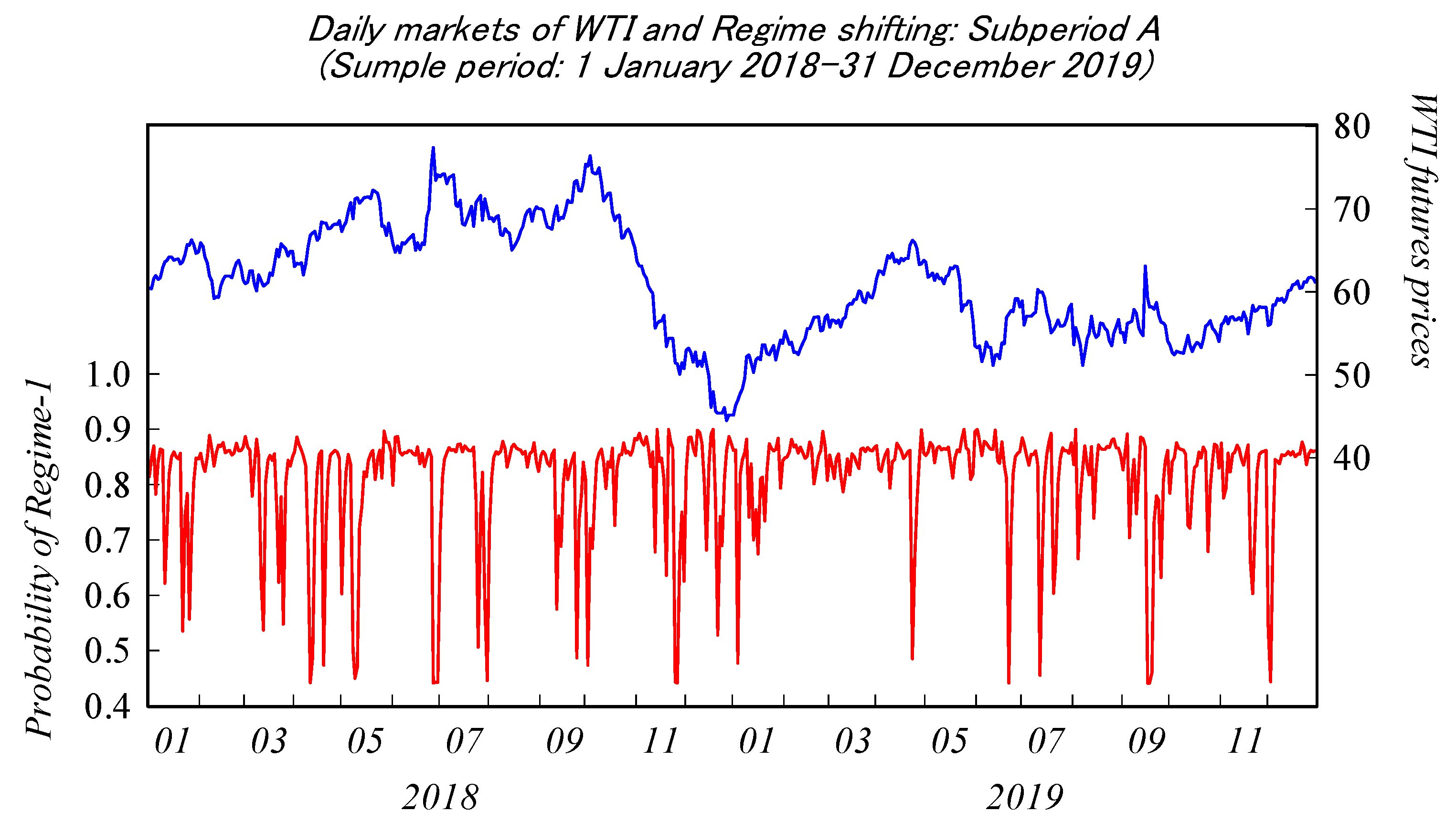
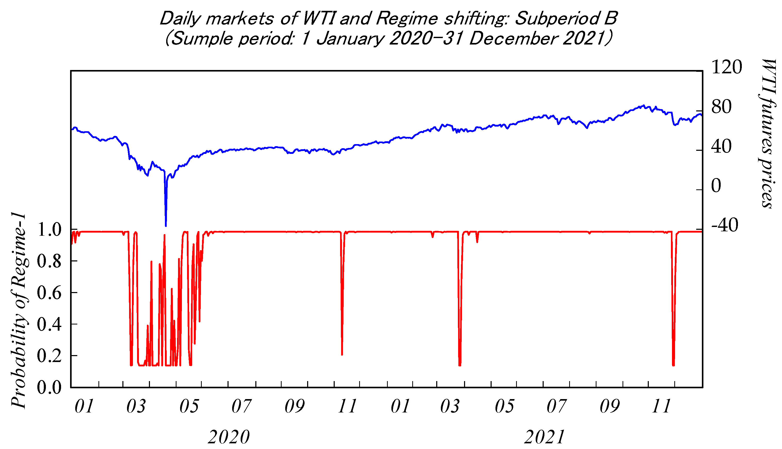
Thus, the graphical evidence from Figure 2 suggests that regime shifts are more likely to occur frequently during periods of decreasing WTI futures prices and higher economic uncertainty. In order to examine the non-linear dynamics prior to and during the disease outbreak, the model Equation (2) with a two-state Markov chain is estimated for both subperiod A from January 2018 to December 2019 and subperiod B from January 2020 to December 2021. Judging by the results reported in Table 3 for subperiod A, it appears that futures returns are governed by two distinct regimes characterized by different levels of volatility. Regime 1 is associated with a statistically insignificant drift and autoregressive term, as well as an insignificant relationship with equity returns, but with negative correlations with changes in the OVX volatility index and in the dollar index. Though the latter is significant only at the ten-percent level, it is found to be insignificant under the alternative regime. Indeed, futures returns are characterized, under Regime 2, by positive drift and positive correlation with equity returns, albeit significant only at the ten-percent and five-percent levels, respectively.
There is also evidence that Regime 2 implies mean reversion and a positive correlation with changes in the OVX index. In contrast to Regime 1 and to both regimes for the full sample period, the significance of the β 2 coefficient suggests that futures returns tend instead to rise in association with increasing uncertainty. This is consistent with the evidence from Aboura and Chevallier (2013), who found a positive correlation between changes in OVX levels and oil prices in association with the onset of the U.S. credit crisis. Judging from the tests of null hypotheses for equal regression coefficients, it appears that the Markov regimes can be distinguished not so much on the basis of differences in the correlations with currency and equity returns as differences between autoregressive terms and correlation with volatility expectations.
With respect to the estimation results for subperiod B, also reported in Table 3, there is clear evidence that the behavior of oil futures returns is likely to be governed by two Markov regimes that tend to differ only on the basis of weaker and stronger correlation with changes in the OVX index. Indeed, the drift terms for both regimes are associated with positive signs but statistically significant only for Regime 1 at the ten-percent level. Additionally, the autoregressive terms are found to be statistically insignificant for both regimes. The relationship of futures returns with the dollar index returns is found to be negative at the five-percent level for Regime 1 but insignificant for Regime 2. Similarly, the regression coefficient δ s reflecting the sensitivity of futures returns to changes in equity valuation is found to be positive under Regime 1 but insignificant under the alternative regime. It is clear that only the regression coefficients β s are found to be negative and significant at the one-percent level under both regimes. Thus, a shift from Regime 1 is likely to be accompanied by a strong increase in sensitivity to changes in volatility expectations under Regime 2.
Judging by the estimated probability values reported in Figure 3, it is Regime 1 that seems to predominate over subperiod A. The regime switches are not likely to take place as the decrease in the likelihood of Regime 1 remains above the fifty-percent threshold probability value. Thus, it is the Regime with a strong negative correlation with volatility expectations that is more likely to prevail. Similarly, the evidence from Figure 4, which reports the Regime 1 probability for subperiod B, suggests that there are frequent regime shifts in association with the precipitous fall in futures prices below zero. A shift toward Regime 2 implies that future returns are governed by a stronger negative correlation with changes in the OVX index. This suggests that higher levels of volatility expectations are conducive to even lower futures returns. Apart from the short period of negative future pricing, it is Regime 1 that tends to prevail with a weaker but still significantly negative correlation with volatility expectations.
In order to further examine the robustness of two-state Markov-regime switching models to changes in the sample period, the focus is made on subperiod C from July 2008 to June 2010, which may be in part reflective of the effects of the U.S. credit crisis on the inner dynamics of oil futures returns and their relationship with volatility expectations and alternative asset markets. The evidence from Table 4, which reports the estimation of the regime-switching model with a two-state Markov chain, indicates that both regimes are characterized by statistically insignificant drifts ω s and autoregressive terms α s . However, futures returns are likely to be governed by strong negative correlation with dollar index returns γ s and positive correlations with equity returns δ s under both regimes. In contrast, a shift from Regime 1 to Regime 2 is likely to result in a strong negative correlation between futures returns and volatility expectations fading away. However, the aggregate evidence from Wald tests of the null hypothesis of equal coefficients suggests that it is difficult to distinguish between these Markov regimes and that, given their similar properties, it is more likely that the two regimes collapse into a single one with significantly negative sensitivity to dollar index returns γ < 0 , positive sensitivity to δ > 0 , and a more likely negative correlation with changes in the OVX index β 0 . Thus, it is clear from the estimation results for subperiod C that periods of financial instability can weaken the correlation of futures returns with volatility expectations. Under higher levels of uncertainty, an increase in oil volatility expectations may not be conducive to diminishing futures returns. It is rather the linkage between oil futures returns and financial markets that gains more significance. Increasing oil futures returns are more likely to result from lower dollar valuation and higher equity.

4.3. Robustness Checks

This paper assumes that there is two-state, lower volatility under bullish markets and higher volatility under bearish markets, in the WTI futures market that reflects market uncertainty and conducts an empirical analysis using the Markov-regime switching model (a non-linear model) to determine whether the correlation between WTI returns and OVX daily change performs with a two-state view of the market depending on the fluctuation of markets. Furthermore, it is possible to consider empirical analysis from a different perspective without taking into account the inner market states. The approach uses a linear model to analyze the correlation between WTI returns and OVX daily fluctuations before and after the structural change date, respectively. Thus, in this section, it is used the autoregressive distributed lag (ARDL) model, one of the linear models, to test whether the empirical analysis demonstrated in this paper is robust. This section also examines whether especially WTI and OVX have a cointegration relationship in each period before and after the structural change using the bounds-testing approach of Pesaran et al. (2001).
In the first place, an explanation of the empirical model used in the linear model estimation is provided. Equation (10) is based on the general ARDL model and incorporates variables similar to those in Equation (2) used in this paper.
y W T I , t = ω + k = 1 m α k y W T I , t k + k = 0 m β k y O V X , t k + k = 0 m γ k y U S D , t k + k = 0 m δ k y S P X , t k + ε t
where the disturbance terms are white noise distributed with ε t ~ i . i . d . N ( 0 , σ 2 ) . m is lag up to 1, 2, …, 8, where m is selected as the optimal lag length by the AIC. Then, in order to estimate whether all variables, WTI returns, OVX daily changes, dollar index daily changes, and S&P 500 index returns, have a long-run relationship, an extension is made from Equation (10) to Equation (11), following the method derived by Pesaran et al. (2001). Equation (11) can be expressed as follows:
Δ y W T I , t = a 0 + i = 1 m a 1 , i Δ y W T I , t i + i = 0 m a 2 , i Δ y O V X , t i + i = 0 m a 3 , i Δ y U S D , t i + i = 0 m a 4 , i Δ y S P X , t i + a 5 y W T I , t 1 + a 6 y O V X , t 1   + a 7 y U S D , t 1 + a 8 y S P X , t 1 + ε t
where Δ is the first difference operator, a 0 , a 1 , a 2 ,…, a 7 , and a 8 are parameters, m is the optimal lag length to be used for estimation selected by AIC. The bounds-testing approach is based on the F-Statistic and is the first of the ARDL cointegration methods. The null hypothesis test of no cointegration, ( H 0 :   a 5 = a 6 = a 7 = a 8 = 0 ), will be performed by Equation (11). Following Pesaran et al. (2001), it is computed two sets of critical values for a given significance level. One set assumes that all variables are I(0), and the other set assumes all variables are I(1). There are three cases that will be obtained. In case one, if the estimated F-Statistic exceeds the upper critical value, the null hypothesis is rejected. In case two, if the estimated F-Statistic is between the upper critical value and lower critical value, then the testing becomes inconclusive. In case three, if the estimated F-Statistic is below the lower critical value, it suggests no cointegration among all variables.
As noted in Section 4.2, the result from the Chow test for structural breaks indicates that the date on which the existence of structural break is 25 December 2019, and it can be regarded as approximately equal to the base point of dividing subperiods A and B. Therefore, it is performed estimation using Equations (10) and (11) in sub-periods A and B to verify the change in the correlation between WTI returns and OVX daily changes before and after a structural change and to test whether there is a long-run relationship between all variables.
Table 5 summarizes the results estimated in subperiod A using Equation (10), which reflects the optimal lag length selected by AIC, and the results of the bounds test for examining the long-run relationship between all variables using Equation (11). The estimated result with Equation (10) for subperiod A indicates that contemporaneous to three periods earlier, OVX daily changes are weakly negatively correlated with WTI returns. The absolute value of the t-value is the largest for the contemporaneous OVX daily change, suggesting that the contemporaneous period of OVX daily changes is more influential than the other lags to WTI returns where time t. Additionally, the results of the bounds testing with Equation (11) indicate that the estimated F-Statistic exceeds the upper critical value, which means that it has rejected the no levels of relationship at the 1% significance level (F-Statistic), suggesting there is a cointegration relationship between all variables in subperiod A.
On the other hand, Table 6, which reports the results estimated in subperiod B using Equation (10) reflecting the optimal lag length selected by AIC, shows that only the contemporaneous OVX daily change is strongly negatively correlated with the WTI return, and the absolute value of the t value is larger than the other variables, the dollar index daily change and S&P 500 returns, suggesting that the contemporaneous period of OVX daily changes is more influential than the other lags and variables to WTI returns where time t. Table 6 also reports the results of the bound test with Equation (11). As in subperiod A, the result indicates that the estimated F-Statistic exceeds the upper critical value, which means that it has rejected the no levels of relationship at the 1% significance level (F-Statistic), suggesting there is also a cointegration relationship between all variables in subperiod B.
From the estimation results for subperiods A and B using the linear ARDL model, it can be observed that the correlation between WTI returns and OVX daily changes changed with the occurrence of COVID-19, which is consistent with the empirical results in this paper. In addition, the fact that a cointegration relationship is established in both subperiods from the results of using Pesaran et al.’s (2001) bounds test suggests that even with structural changes, there is the long-run relationship, which is an important point in the crude oil market. Thus, the empirical results of this paper can be regarded as robust because the change in the correlation between WTI returns and OVX daily changes before and after the structural change can also be observed in the estimation using the linear model and is consistent with the results of this paper.

5. Conclusions

The present study provides new empirical evidence on the stochastic behavior of energy futures returns based on the estimation of Markov-regime switching models. Given the nature of energy markets, the demand and supply functions are intrinsically linked with the real economy and perceptions of economic uncertainty, but there is growing literature about stronger linkages with the financial economy as well. The focus of this paper is placed on the empirical issue of whether the inner dynamics and correlation structures of oil futures with alternative asset markets are governed by different regimes that reflect changes in the underlying demographic, macroeconomic and social conditions. The empirical evidence suggests that oil futures returns tend to be governed by different Markov regimes, which invariably exhibit a negative correlation with volatility expectations which reflect the shifting fear factor dynamics. Thus, market perceptions of heightened economic uncertainty reflected by increased volatility expectations are conducive to diminishing futures returns, irrespective of the prevailing regime.
The non-linear dynamics of oil futures returns can be altered, however, by significant events such as the onset of financial crises and disease outbreaks, as well as government policy responses. There is, indeed, evidence that the economic lockdowns in response to the disease outbreak have the potential to increase the likelihood of Markov regimes with a more pronounced negative correlation of futures returns with changes in expected volatility. Additionally, periods of financial instability, such as the U.S. credit crisis, may sever the relationship of oil futures returns with volatility expectations and strengthen their linkages with currency fluctuations and equity valuation. Thus, Markov-regime switching models have the capacity to capture changes in the underlying fundamentals and provide some insights into the changing inner dynamics, such as the propensity for mean reversion and a long memory for economic shocks that tend to decay over a longer time. Regrettably, this paper’s shortcomings include the fact that the Markov-regime switching model does not resolve the issues of strict simultaneity and endogeneity between WTI and OVX, which is an issue for future research. Further research may shed light on the non-linear dynamics with time-varying transition probabilities, simultaneity, and jump-diffusion processes which may better account for the stochastic properties of energy prices.

Funding

This research received no external funding.

Data Availability Statement

The data presented in this paper are available upon request from the author. All time-series data used in the analysis in this paper can be obtained from the Thomson Reuters database.

Acknowledgments

I would like to express my appreciations to the three anonymous reviewers who reviewed my paper, to Kentaro Iwatsubo from Kobe University for his comments this paper and Nabil Maghrebi from Wakayama University for proofreading the English text.

Conflicts of Interest

The author declares no conflict of interest.

Notes

1
It is noted that the study by Fleming et al. (1995) was performed with a volatility index based on the S&P 100 stock market index, formerly known as VIX index.
2
The focus is also placed, as in Mencia and Sentana (2013), on the valuation of VIX derivatives, where the volatility index serves as the underlying asset for derivatives contracts.
3

References

  1. Aboura, Sofiane, and Julien Chevallier. 2013. Leverage vs. feedback: Which Effect drives the oil market? Finance Research Letters 10: 131–41. [Google Scholar] [CrossRef] [Green Version]
  2. Baiardi, Lorenzo Cerboni, Massimo Costabile, Domenico De Giovanni, Fabio Lamantia, Arturo Leccadito, Ivar Massabó, Massimiliano Menzietti, Marco Pirra, Emilio Russo, and Alessandro Staino. 2020. The Dynamics of the S&P 500 under a crisis context: Insights from a Three-Regime Switching Model. Risks 8: 71. [Google Scholar]
  3. Baumeister, Christian, and Lutz Kilian. 2012. Real-Time Forecasts of the Real Price of Oil. Journal of Business & Economic Statistics 30: 326–36. [Google Scholar]
  4. Baumeister, Christian, and Lutz Kilian. 2015. Forecasting the Real Price of Oil in a Changing World: A Forecast Combination Approach. Journal of Business & Economic Statistics 33: 338–51. [Google Scholar]
  5. Beckmann, Joscha, Robert L. Czudaj, and Vipin Arora. 2020. The relationship between oil prices and exchange rates: Revisiting theory and evidence. Energy Economics 88: 104772. [Google Scholar] [CrossRef]
  6. Bodie, Zvi, and Victor I. Rosansky. 1980. Risk and Return in Commodity Futures. Financial Analysts Journal 36: 27–39. [Google Scholar] [CrossRef]
  7. Chen, Yanhui, Kaijian He, and Lean Yu. 2015. The Information Content of OVX for Crude Oil Returns Analysis and Risk Measurement: Evidence from the Kalman Filter Model. Annals of Data Science 2: 471–87. [Google Scholar] [CrossRef] [Green Version]
  8. Cheng, Ing-Haw, and Wei Xiong. 2014. Financialization of Commodity Market. Annual Review of Financial Economics 6: 419–41. [Google Scholar] [CrossRef] [Green Version]
  9. Cheung, C. Sherman, and Peter Miu. 2010. Diversification benefits of commodity futures. Journal of International Financial Markets, Institutions and Money 20: 451–74. [Google Scholar] [CrossRef]
  10. Choi, K., and S. Hammoudeh. 2010. Volatility behavior of oil, industrial commodity and stock markets in a regime-switching environment. Energy Policy 38: 4388–99. [Google Scholar] [CrossRef]
  11. Connolly, Robert A., Chris Stivers, and Licheng Sun. 2005. Stock Market Uncertainty and the Stock-Bond Return Relation. Journal of Financial and Quantitative Analysis 40: 161–94. [Google Scholar] [CrossRef] [Green Version]
  12. Creti, Anna, Marc Joëts, and Valérie Mignon. 2013. On the links between stock and commodity markets’ volatility. Energy Economics 37: 16–28. [Google Scholar] [CrossRef] [Green Version]
  13. Diebold, Francis X., Joon-Haeng Lee, and Gretchen C. Weinbach. 1994. Regime switching with time-varying transition probabilities. In Advanced Texts in Econometrics. Edited by Clive William John Granger and Grayham Mizon. Oxford: Oxford University Press, pp. 283–302. [Google Scholar]
  14. Dupoyet, Brice V., and Corey A. Shank. 2018. Oil prices implied volatility or direction: Which matters more to financial markets? Financial Markets and Portfolio Management 32: 275–95. [Google Scholar] [CrossRef]
  15. Dutta, Anupam. 2017. Oil price uncertainty and clean energy stock returns: New evidence from crude oil volatility index. Journal of Cleaner Production 164: 1157–66. [Google Scholar] [CrossRef]
  16. Federal Reserve Board. 2022. Financial Stability Report; Washington, DC: The United States of America Board of Governors of The Federal Reserve System, May 9.
  17. Ferraro, Domenico, Kenneth Rogoff, and Barbara Rossi. 2015. Can oil prices forecast exchange rates? An empirical analysis of the relationship between commodity prices and exchange rates. Journal of International Money and Finance 54: 116–41. [Google Scholar] [CrossRef]
  18. Filardo, Andrew J. 1994. Business cycle phases and their transitions. Journal of Business and Economic Statistics 12: 299–308. [Google Scholar]
  19. Fleming, Jeff, Barbara Ostdiek, and Robert E. Whaley. 1995. Predicting stock market volatility: A new measure. The Journal of Futures Markets 15: 265–302. [Google Scholar] [CrossRef]
  20. Fukasawa, Masaaki, Isao Ishida, Nabil Maghrebi, Kosuke Oya, Masato Ubukata, and Kazutoshi Yamazaki. 2011. Model-free implied volatility: From surface to index. International Journal of Theoretical and Applied Finance 14: 433–63. [Google Scholar] [CrossRef]
  21. Giot, Pierre. 2003. The Asian Financial Crisis: The Start of a Regime Switch in Volatility. CORE Discussion Paper, No.2003/78. Rochester: SSRN. [Google Scholar]
  22. Goldstein, Itay, and Liyan Yang. 2022. Commodity Financialization and Information Transmission. The Journal of Finance 77: 2613–67. [Google Scholar] [CrossRef]
  23. Gong, Xu, and Jun Xu. 2022. Geopolitical risk and dynamic connectedness between commodity markets. Energy Economics 110: 106028. [Google Scholar] [CrossRef]
  24. Gorton, Gary, and K. Geert Rouwenhorst. 2006. Facts and Fantasies about Commodity Futures. Financial Analysts Journal 62: 47–68. [Google Scholar] [CrossRef] [Green Version]
  25. Grima, Simon, Letife Özdemir, Ercan Özen, and Inna Romānova. 2021. The Interactions between COVID-19 Cases in the USA, the VIX Index and Major Stock Markets. International Journal of Financial Studies 9: 26. [Google Scholar] [CrossRef]
  26. Hamilton, James D. 1989. A New approach to the economic analysis of nonstationary time series and the business cycle. Econometrica 57: 357–84. [Google Scholar] [CrossRef]
  27. Hamilton, James D. 1994. Time Series Analysis. Princeton: Princeton University Press. [Google Scholar]
  28. Hamilton, James D. 2008. Understanding Crude Oil Prices. National Bureau of Economic Research Working Paper, No. 14492. Cambridge: National Bureau of Economic Research. [Google Scholar]
  29. Harris, Glen R. 1999. Markov chain Monte Carlo estimation of regime switching vector autoregressions. Austin Bulletin 29: 47–79. [Google Scholar] [CrossRef]
  30. Jensen, Gerald R., Robert R. Jhonson, and Jeffrey M. Mercer. 2000. Efficient use of commodity futures in diversified portfolios. The Journal of Futures Markets 20: 489–506. [Google Scholar] [CrossRef]
  31. Just, Małgorzata, and Krzysztof Echaust. 2020. Stock market returns, volatility, correlation and liquidity during the COVID-19 crisis: Evidence from the Markov Switching approach. Finance Research Letters 37: 101775. [Google Scholar] [CrossRef]
  32. Kim, Chang-Jin, Jeremy M. Piger, and Richard Startz. 2008. Estimation of Markov regime-switching regression models with endogenous switching. Journal of Econometrics 143: 263–73. [Google Scholar] [CrossRef] [Green Version]
  33. Kim, Suyi, So-Yeun Kim, and Kyungmee Choi. 2019. Analyzing oil price shocks and exchange rates movements in Korea using Markov Regime-Switching models. Energies 12: 4581. [Google Scholar] [CrossRef] [Green Version]
  34. Liu, Bing-Yue, Qiang Ji, and Ying Fan. 2017. Dynamic return-volatility dependence and risk measure of CoVaR in the oil market: A time-varying mixed copula model. Energy Economics 68: 53–65. [Google Scholar] [CrossRef]
  35. Lombardi, Marco, and Francesco Ravazzolo. 2013. On the Correlation between Commodity and Equity Returns: Implications for Portfolio Allocation. BIS Working Papers No, 420. Basel: Bank for International Settlements. [Google Scholar]
  36. MacKinnon, James G. 1996. Numerical Distribution Function for Unit root and Cointegration tests. Journal of Applied Econometrics 11: 601–18. [Google Scholar] [CrossRef]
  37. Maghrebi, Nabil, Moo-Sung Kim, and Kazuhiko Nishina. 2007. The Kospi 200 Implied Volatility Index: Evidence of Regime Switches in Volatility Expectations. Asia-Pacific Journal of Financial Studies 36: 163–87. [Google Scholar]
  38. Maghrebi, Nabil, Mark J. Holmes, and Kosuke Oya. 2014. Financial instability and the short-term dynamics of volatility expectations. Applied Financial Economics 24: 377–95. [Google Scholar] [CrossRef]
  39. Mencia, Javier, and Enrique Sentana. 2013. Valuation of VIX derivatives. Journal of Financial Economics 108: 367–91. [Google Scholar] [CrossRef] [Green Version]
  40. Mensi, Walid, Makram Beljid, Adel Boubaker, and Shunsuke Managi. 2013. Correlations and volatility spillovers across commodity and stock markets: Linking energies, food, and gold. Economic Modelling 32: 15–22. [Google Scholar] [CrossRef] [Green Version]
  41. Nishina, Kazuhiko, Nabil Maghrebi, and Moo-Sung Kim. 2006. Stock Market Volatility and the Forecasting Accuracy of Implied Volatility Indices. Discussion Papers in Economics and Business No. 06-09. Toyonaka: Graduate School of Economics and Osaka School of International Public Policy. [Google Scholar]
  42. Nishina, Kazuhiko, Nabil Maghrebi, and Mark J. Holmes. 2012. Nonlinear Adjustments of Volatility Expectations to Forecast Errors: Evidence from Markov-Regime Switches in Implied Volatility. Review of Pacific Basin Financial Markets and Policies 15: 1250007. [Google Scholar] [CrossRef]
  43. Pesaran, M. Hashiem, Yongcheol Shin, and Richard J. Smith. 2001. Bounds Testing Approaches to the Analysis of Level Relationships. Journal of Applied Econometrics 16: 289–326. [Google Scholar] [CrossRef]
  44. Pindyck, Robert S. 2001. The dynamics of commodity spot and futures markets: A Primer. The Energy Journal 22: 1–29. [Google Scholar] [CrossRef] [Green Version]
  45. Pouzo, Demian, Zacharias Psaradakis, and Martin Sola. 2022. Maximum likelihood estimation in Markov regime-switching models with covariate-dependent transition probabilities. Econometrica 90: 1681–710. [Google Scholar] [CrossRef]
  46. Raza, Naveed, Syed Jawad Hussain Shahzad, Aviral Kumer Tiwari, and Muhammad Shahbaz. 2016. Asymmetric impact of gold, oil prices and their volatilities on stock prices of emerging markets. Resources Policy 49: 290–301. [Google Scholar] [CrossRef]
  47. Sarwar, Ghulam. 2012. Is VIX an investor fear gauge in BRIC equity markets? Journal of Multinational Financial Management 22: 55–65. [Google Scholar] [CrossRef]
  48. Silvennoinen, Annastiina, and Susan Thorp. 2013. Financialization, crisis and commodity correlation dynamics. Journal of International Financial Markets, Institutions and Money 24: 42–65. [Google Scholar] [CrossRef] [Green Version]
  49. Smales, Lee A. 2022. Spreading the fear: The central role of CBOE VIX in global stock market uncertainty. Global Finance Journal 51: 100679. [Google Scholar] [CrossRef]
  50. Szado, Edward. 2009. VIX Futures and options: A Case Study of Portfolio Diversification During the 2008 Financial Crisis. The Journal of Alternative Investments 12: 68–85. [Google Scholar] [CrossRef]
  51. Tang, Ke, and Wei Xiong. 2012. Index Investment and the Financialization of Commodities. Financial Analysts Journal 68: 54–74. [Google Scholar] [CrossRef]
  52. Wang, Gang-Jin, and Chi Xie. 2012. Cross-correlations between WTI crude oil market and U.S. stock market: A perspective from econophysics. Acta Physica Polonica B 43: 10. [Google Scholar] [CrossRef]
  53. Whaley, Robert E. 2000. The investor fear gauge. Journal of Portfolio Management 26: 12–17. [Google Scholar] [CrossRef]
  54. Whaley, Robert E. 2009. Understanding the VIX. The Journal of Portfolio Management 35: 98–105. [Google Scholar] [CrossRef]
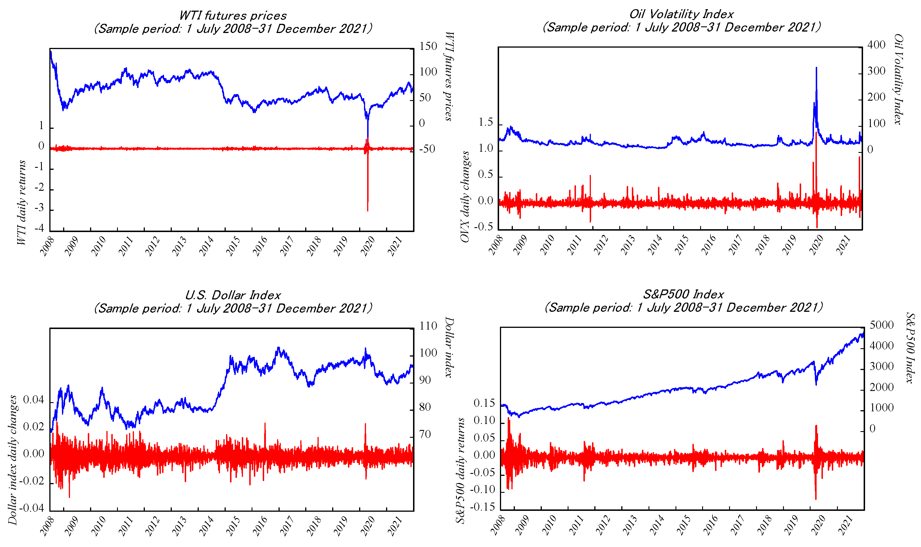
Figure 1. The behavior of price levels and returns in WTI futures, OVX, dollar index, and equity markets.
Jrfm 16 00067 g001
Figure 2. Probability of Regime 1 (Full sample period July 2008–December 2021).
Jrfm 16 00067 g002
Figure 3. Probability of Regime 1 (Subperiod A—January 2018–December 2021).
Jrfm 16 00067 g003
Figure 4. Probability of Regime 1 (Subperiod B—January 2020–December 2021).
Jrfm 16 00067 g004
Table 1. Distributional Properties.
Distributional
Moments
MeanStd.
Dev.
SkewnessKurtosisJarque
Bera
ADF Test
WTI returns −0.0007 0.062728 −33.5240 1569.688 3.61 × 10⁸ −43.544 ***b
OVX daily changes 0.00174 0.063033 4.9582 87.09921 1,052,944.0 −61.760 ***a
Dollar index daily changes 0.00009 0.004761 −0.0492 5.870737 1211.493 −58.464 ***b
S&P 500 returns 0.00045 0.012766 −0.2904 17.14844 29,442.39 −68.718 ***a
Notes: The sample period of daily observation runs from 1 July 2008, to 31 December 2021. Significance at the 1% level is denoted by asterisks *** under MacKinnon (1996)’s one-sided probability values. The stationarity of time series is estimated with the Augmented Dickey–Fuller methodology using the intercept only and with neither intercept nor trend terms as denoted by superscripts a and b respectively. Jarque–Bera statistics for normal tests are distributed as χ 2 on the null.
Table 2. Markov-regime switching model results (Full estimated period).
Model ParametersFull Period (July 2008–December 2021)
Markov-Regime 1Markov-Regime 2
ω −0.0001
(0.6697)
0.0174
(0.2269)
α −0.0196
(0.1708)
0.1592 ***
(0.0045)
β −0.1452 ***
(0.0000)
−0.9643 ***
(0.0000)
γ −0.8659 ***
(0.0000)
−1.4004
(0.4340)
δ 0.3820 ***
(0.0000)
−0.6599
(0.2359)
L o g ( σ ) −4.1048 ***
(0.0000)
−1.6497 ***
(0.0000)
Log likelihood 9124.611
AIC −4.9880
Hypothesis Tests
ω 1 = ω 2 1.4408
(0.2300)
α 1 = α 2 9.5865 ***
(0.0020)
β 1 = β 2 76.7273 ***
(0.0000)
γ 1 = γ 2 0.0259
(0.8723)
δ 1 = δ 2 3.2807 *
(0.0701)
Notes: The estimated Markov-regime Switching model is represented by equation: y W T I , t = ω s t + α s t y W T I , t 1 + β s t y O V X , t + γ s t y U S D , t + δ s t y S P X , t + ε t . The sample period of daily observation runs from 1 July 2008 to 31 December 2021. Significance at 1 and 10% level is denoted by *** and *, respectively. The hypothesis tests for equal coefficients are based on the Wald test following the χ2 distribution. Figures in round brackets represent probability values.
Table 3. Results of Subperiod A and B estimated with Markov-regime switching modeling.
Model Parameters Subperiod A
(January 2018–December 2019)
Subperiod B
(January 2020–December 2021)
Regime 1 Regime 2 Regime 1 Regime 2
ω −0.0009
(0.2648)
0.0056 *
(0.0811)
0.0014 *
(0.0835)
0.0135
(0.7792)
α 0.0145
(0.7738)
−2.4246 **
(0.0153)
0.0014
(0.9667)
0.1383
(0.1553)
β −0.2205 ***
(0.0000)
0.2100 ***
(0.0000)
−0.1802 ***
(0.0000)
−1.2691 ***
(0.0000)
γ −0.4526 *
(0.0671)
−0.1772
(0.8440)
−0.5188 **
(0.0379)
−2.3555
(0.7371)
δ 0.0913
(0.3084)
0.8216 **
(0.0488)
0.2888 ***
(0.0003)
−1.9662
(0.1892)
L o g ( σ ) −4.3179 ***
(0.0000)
−3.7329 ***
(0.0000)
−4.1164 **
(0.0000)
−1.1437 ***
(0.0000)
Log Likelihood 1403.674 1219.407
AIC −5.324421 −4.609587
Hypothesis tests
ω 1 = ω 2 3.4875 *
(0.0618)
0.0636
(0.8009)
α 1 = α 2 4.3483 **
(0.0370)
1.7564
(0.1851)
β 1 = β 2 84.6471 ***
(0.0000)
38.8884 ***
(0.0000)
γ 1 = γ 2 0.0783
(0.7796)
0.0684
(0.7936)
δ 1 = δ 2 2.6231
(0.1053)
2.2305
(0.1353)
Notes: The estimated Markov-regime Switching model is represented by the equation: y W T I , t = ω s t + α s t y W T I , t 1 + β s t y O V X , t + γ s t y U S D , t + δ s t y S P X , t + ε t . The sample period of daily observation runs from 1 January 2018 to 31 December 2021. Significance at the 1, 5, and 10% levels is denoted by ***, **, and *, respectively. The hypothesis tests for equal coefficients are based on the Wald test following the χ 2 distribution. Figures in round brackets represent probability values.
Table 4. Markov-regime switching model results (Subperiod C estimated period).
Model ParametersSubperiod C (July 2008–June 2010)
Markov-Regime 1Markov-Regime 2
ω 0.0006
(0.4797)
−0.0008
(0.8519)
α 0.0621
(0.1126)
−0.0018
(0.8062)
β −0.1402 ***
(0.0000)
−0.0958
(0.1062)
γ −1.7029 ***
(0.0000)
−1.1439 **
(0.0169)
δ 0.3553 ***
(0.0000)
0.4894 ***
(0.0006)
L o g ( σ ) −4.1663 ***
(0.0000)
−2.9762 ***
(0.0000)
Log likelihood 1220.131
AIC −4.6212
Hypothesis Tests
ω 1 = ω 2 0.1054
(0.7454)
α 1 = α 2 0.8807
(0.3480)
β 1 = β 2 0.3969
(0.5287)
γ 1 = γ 2 1.0965
(0.2950)
δ 1 = δ 2 0.5650
(0.4523)
Notes: The estimated Markov-regime Switching model is represented by the equation: y W T I , t = ω s t + α s t y W T I , t 1 + β s t y O V X , t + γ s t y U S D , t + δ s t y S P X , t + ε t . The sample period of daily observation runs from 1 July 2008 to 30 June 2010. Significance at the 1 and 5% levels is denoted by *** and **, respectively. The hypothesis tests for equal coefficients are based on the Wald test following the χ 2 distribution. Figures in round brackets represent probability values.
Table 5. Results of Subperiod A estimated with ARDL modeling and the bounds test.
Model Parameters
[ARDL (5,3,2,0)]
Subperiod A (January 2018–December 2019)
Coefficientt-Statistic
ω 0.00070.8380
α t 1 −0.1567 ***−3.5950
α t 2 −0.0658−1.4974
α t 3 −0.0814 *−1.8818
α t 4 0.05821.4148
α t 5 0.0733 *1.7949
β t −0.1010 ***−6.2670
β t 1 −0.0648 ***−4.0226
β t 2 −0.0360 **−2.2070
β t 3 −0.0317 *−1.9481
γ t −0.2385−0.9302
γ t 1 −0.5504 **−2.1447
γ t 2 −0.4391 *−1.7066
δ t 0.2806 ***2.9526
Log Likelihood1340.482
AIC−5.0823
F-Bounds Test (At the 1% significance level)
F-StatisticI(0)I(1)
29.92583.654.66
Notes: The estimated ARDL model is represented by Equation (10): y W T I , t = ω + k = 1 m α k y W T I , t k + k = 0 m β k y O V X , t k + k = 0 m γ k y U S D , t k + k = 0 m δ k y S P X , t k + ε t . The sample period of daily observation runs from 1 January 2018 to 31 December 2019. Significance at the 1, 5, and 10% levels is denoted by ***, **, and *, respectively. The hypothesis test of cointegration for all variables is based on the bounds testing with Equation (11): Δ y W T I , t = a 0 + i = 1 m a 1 , i Δ y W T I , t i + i = 0 m a 2 , i Δ y O V X , t i + i = 0 m a 3 , i Δ y U S D , t i + i = 0 m a 4 , i Δ y S P X , t i + a 5 y W T I , t 1 + a 6 y O V X , t 1 + a 7 y U S D , t 1 + a 8 y S P X , t 1 + ε t .
Table 6. Results of Subperiod B estimated with ARDL modeling and the bounds test.
Model Parameters
[ARDL (4,0,4,1)]
Subperiod B (January 2020–December 2021)
Coefficientt-Statistic
ω 0.00370.7861
α t 1 0.2494 ***7.2207
α t 2 −0.1279 ***−3.6187
α t 3 0.04001.1396
α t 4 0.0577 *1.7318
β t −0.8823 ***−18.6752
γ t −1.2195−0.9081
γ t 1 0.55920.4318
γ t 2 −1.5832−1.2145
γ t 3 −3.7311 ***−2.8466
γ t 4 3.2288 **2.4446
δ t −1.4937 ***−4.2291
δ t 1 −1.5759 ***−4.5938
Log Likelihood426.7656
AIC−1.5823
F-Bounds Test (At the 1% significance level)
F-StatisticI(0)I(1)
109.63503.654.66
Notes: The estimated ARDL model is represented by Equation (10): y W T I , t = ω + k = 1 m α k y W T I , t k + k = 0 m β k y O V X , t k + k = 0 m γ k y U S D , t k + k = 0 m δ k y S P X , t k + ε t . The sample period of daily observation runs from 1 January 2020 to 31 December 2020. Significance at the 1, 5, and 10% levels is denoted by ***, **, and *, respectively. The hypothesis test of cointegration for all variables is based on the bounds testing with Equation (11): Δ y W T I , t = a 0 + i = 1 m a 1 , i Δ y W T I , t i + i = 0 m a 2 , i Δ y O V X , t i + i = 0 m a 3 , i Δ y U S D , t i + i = 0 m a 4 , i Δ y S P X , t i + a 5 y W T I , t 1 + a 6 y O V X , t 1 + a 7 y U S D , t 1 + a 8 y S P X , t 1 + ε t .
Disclaimer/Publisher’s Note: The statements, opinions and data contained in all publications are solely those of the individual author(s) and contributor(s) and not of MDPI and/or the editor(s). MDPI and/or the editor(s) disclaim responsibility for any injury to people or property resulting from any ideas, methods, instructions or products referred to in the content.