Abstract
We derive the explicit price of the perpetual American put option canceled at the last-passage time of the underlying above some fixed level. We assume that the asset process is governed by a geometric spectrally negative Lévy process. We show that the optimal exercise time is the first moment when the asset price process drops below an optimal threshold. We perform numerical analysis considering classical Black–Scholes models and the model where the logarithm of the asset price has additional exponential downward shocks. The proof is based on some martingale arguments and the fluctuation theory of Lévy processes.
Keywords:
American options; optimal stopping problem; Lévy process; last passage time; free boundary problem MSC:
60G40; 60J75; 91G80
1. Introduction
The main goal of this paper is to find the closed-form formula for the price of the perpetual American put option canceled at the last-passage time of the underlying above some fixed level h. More formally, in this paper, we find the following value function
for a family of stopping times , an underlying risky asset price process , fixed strike price and the risk-free interest rate r, where
for some fixed threshold . We assume a Lévy market, that is, in our model, the asset price is described by a geometric spectrally negative Lévy process
where is a spectrally negative Lévy process and is an initial asset price. It is well known that a Lévy market allows for a more realistic representation of price dynamics, capturing certain features such as skewness and asymmetry, as well as a greater flexibility in calibrating the model to market prices; see, e.g., Cont (2001); Cont and Tankov (2004) and references therein.
In fact, we choose
where and . In (4), is a Brownian motion, is a fixed drift, is a homogeneous Poisson process (independent of ) with intensity and is a sequence (independent of and ) of independent identically distributed exponential random variables with the expected value . We assume that all considered processes live in a common filtered probability space with a natural filtration of satisfying the usual conditions. The above process (4) makes the asset price process a jump-diffusion model. Furthermore, we assume that dividends are not paid to the holders of the underlying asset and that the expectation in (1) is taken with respect to the martingale measure , that is, is a local martingale. In fact, as noted in (Cont and Tankov 2004, Table 1.1, p. 29), introducing jumps into the model implies a loss of completeness of the market, which results in the lack of uniqueness of an equivalent martingale measure. Still, we can choose one of these measures, and the price is the same regardless of the choice of the martingale measure.
In (4), we allow , which corresponds to the classical Black–Scholes (B-S) model with .
To find the value function (1), we will use the ‘guess and verify method’, in which we guess the candidate stopping rule and then verify that this is truly the optimal stopping rule using the verification Theorem 2. That is, we first guess the form of the stopping time as the first downward crossing time of some threshold and calculate the value function in terms of the scale functions using the fluctuation theory of Lévy processes. Then, we maximize it with respect to the exercise level a. In the last step, we prove that our guessed value function satisfies the Hamilton–Jacobi–Bellman equation (HJB) system and hence the verification step.
In the final part of the paper, we performed a comprehensive numerical analysis based on the known form of the scale functions for the process (4).
The pricing of American options has been investigated over the past four decades in various contexts; see Detemple (2006) for a review. This paper focuses mainly on adding a rather new cancellation feature built into the basic American contract. This canceling or recalling in the financial contracts can effectively mitigate undesirable positions in risky times or times when the markets are highly volatile. Therefore, we believe that this type of financial contract can be very attractive for many investors. Of course, these types of derivatives include a cancellation provision.
Our article continues the research conducted by Gapeev et al. (2020), where the authors also evaluate the American-style option (1), but they carry this out by solving an appropriate HJB system of equations. In Gapeev et al. (2020), the underlying asset price was described by geometric Brownian motion, for which the above approach is very natural due to the locality of the diffusive generator of the asset price process . Still, in the context of nonlocal generators, a ‘guess-and-verify’ method used in this paper seems to be more efficient. To show the relationship of these approaches, we also provide a connection of our results to the seminal HJB equations.
There are other works strongly related to our paper. Most of them reduce the original optimal stopping problems to the associated free boundary problems. Wu and Li (2022) valuate the American put option in a very similar model as Gapeev et al. (2020) did, that is, any stopping rules must be before the last exit time of the price of the underlying assets at any fixed level. This paper focuses only on the Black–Scholes market as well. The difference is that Wu and Li (2022) analyze the finite-time maturity. Gapeev and Motairi (2022) consider the perpetual American cancelable dividend-paying put and call option in the Black–Merton–Scholes market, where the cancellation times are assumed to occur when the underlying risky asset price process hits some unobservable random thresholds. They proved that the optimal stopping times are the first times at which the asset price reaches stochastic boundaries depending on the current values of its running maximum and minimum processes. Other related articles are (Gapeev and Li 2022a, 2022b), who study perpetual American standard and lookback options terminated by the writers at the last times at which the underlying stock reaches its running maximum or minimum. Then, the linear and fractional recovery amounts are paid to the holders. Other important papers are Dumitrescu et al. (2018); Gapeev and Motairi (2018); Gapeev and Rodosthenous (2014); Linetsky (2006); Szimayer (2005) (see also references therein).
2. Main Result
To present the main result of this paper, we introduce required notations. Let be a martingale measure and be the expectation with respect to with the convention . We skip the subindex in expectation when (hence ).
We define a Laplace exponent of the process through
For the process defined in (4), we have
Since under the risk-neutral measure the discounted asset price process is a martingale, we assume throughout this paper that
In other words, we take
For , the so-called scale function is defined as a continuous function such that:
With the first scale function, we associate the second one given by
Lemma 1.
Furthermore,
The proof of this lemma is given in Appendix A. We show that the optimal exercise time is of the form
The threshold a needs to be lower than the strike price K (and hence of the canceling threshold h), so that exercising the option can be profitable to the holder. We take
We denote
The main result of this paper is as follows.
3. Proof of the Main Result
To prove Theorem 1 we start by transforming the value function . Let be the conditional survival process. Additionally, let us introduce a parameter solving
Equation (18) has three solutions. The only one that can be negative is
Observe that . Then,
and
Hence,
where the function G is defined in (16). Representation (20) is very convenient from the point of view of the general optimal stopping theory. However, we can still modify this representation. Observe that by (Ken-Iti 1999, Thm. 31.5, p. 208)
is the infinitesimal generator of the process acting on , where
Due to the localization procedure, is an extended generator that also acts on . For , we denote
where
and denotes the indicator of an event C. Let us also introduce the local time of the process X at the point (see, e.g., Peskir (2007)):
The key representation of is given in the next lemma, for which proof is given in Appendix A.
Lemma 2.
The following holds true:
where
The next step is a verification theorem that allows us to identify . Its proof is also given in Appendix B.
Theorem 2.
Suppose that function , except the point h and a point a, where it is of class . Assume that V satisfies the following HJB system of equations
Then, .
Now, the main idea of the proof of the main result is to find the value function
when the exercise time is the first downward passage time of the asset price defined in (14). We let
for the unique (see assumption (15)) solving and .
In the final step, we show that satisfies all the conditions of the verification theorem (Theorem 2), and therefore we obtain the assertion of the main Theorem 1.
We now prove the following proposition, which is interesting in itself, and its proof is presented in Appendix C.
Proposition 1.
The value is equal to
We are now ready to give the proof of the main result of this paper.
Proof of Theorem 1.
We recall that
for defined in (31) and solving . We verify that the inequality (28) and the Equation (29) formulated in Theorem 2 are satisfied.
By (Kuznetsov 2012, Thm. 3.10), both scale functions and belong to . Hence, by (31), and of class at by the choice of . Moreover,
and hence (29) is satisfied.
Observe that the only candidate for that satisfies condition
is given as a solution of the following equation
and hence is given in (17). We still have to verify if . To do so, we rewrite the representation (17) of as follows:
Furthermore,
and
see also Yamazaki (2017). Therefore, we can see that the right-hand sides of equations in (35) are positive, which means that also the left-hand sides are also positive. As both and are negative, it means that both and are also negative. By virtue of the fact that , we can see that:
This leads to the conclusion that the numerator of the rhs of (34) is strictly positive. Moreover, since and are negative, and , we know that its denominator is negative. This immediately gives . To show that , we need to verify that the numerator plus the denominator is smaller than 0, that is, that
This follows from the fact that are all strictly negative.
Now, note that is a martingale. Indeed, from (Avram et al. 2004, Rem. 5), we know that and are martingales, where . Furthermore, by (A10), the process is a martingale as well, since is martingale, where
is the right-hand side of (A10). To show this, observe that by Markov property of , we have
where we used the fact that for and because due to the assumption that (see (Kuznetsov 2012, Lem. 3.1 and Lem. 3.2)). Since b appearing in above is general, hence
and thus for
by definition (23) of .
Now, for , and . To prove (28), one need thus prove that for . Using the fact that , we can write for in the following form:
Then,
It can easily be seen that the term is strictly positive, as . Additionally, is strictly negative. As both h and s are positive, hence . This completes the proof. □
4. Numerical Analysis
4.1. Geometric Brownian Motion
As the first case in the numerical analysis, we consider the underlying asset price described by the geometric Brownian motion. We set the intensity of the process from Equation (4) equal to zero, and thus becomes the arithmetic Brownian motion with drift parameter . This example corresponds to the option evaluated in Gapeev et al. (2020). The scope of the numerical analysis here is to find the optimal exercise level and the fair price of the option. The parameters are chosen as follows: the strike price , the threshold so that , risk-free rate and the volatility of the underlying asset . Additionally, the initial price of the underlying asset is set to 110. We first start with calculation of . Using formula (17), we obtain . This value fits well to the assumption (15). Furthermore, when we use formula (43) from Gapeev et al. (2020), we obtain the same result:
Now, by using Theorem 1, we obtain the price of the cancelable option . Again, when we use the formula (37) proposed in Gapeev et al. (2020), we obtain the same result:
Now, according to (Wilmott 2006, Chap. 9.2), the price of the standard perpetual American option for the no-dividend case is given by:
where and . The price of this option with parameters chosen as previously in this section is equal to 36.70. This price is significantly higher than the price of the corresponding cancelable option due to the higher risk the issuer of this contract has to deal with.
Finally, in Figure 1, we demonstrate the dependence of the cancelable option price on the initial price of the underlying instrument. Note that the price and payoff function fit smoothly at .
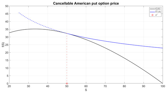
Figure 1.
Smooth fit of the payoff and the price functions for the geometric Brownian motion with parameters: , , , . denotes the value function f where or .
4.2. Geometric Spectrally Negative Lévy Process
Here, we perform a similar calculation as in Section 4.1, but now we set a fixed . We keep the other parameters unchanged, i.e., , and additionally set and . Again, we start by finding the optimal threshold . With formula (17), we obtain . One more time, we use Theorem 1 to find the fair price of the cancelable option, and we obtain . The price is smaller, although it cannot be predicted without numerical analysis. Indeed, although all the jumps of the underlying are downward, the drift is still greater, which is a consequence of applying the martingale measure in a pricing formula.
As the final step, in Figure 2, we show the behavior of the payoff and price functions of the cancelable put option, depending on the initial underlying asset price. Again, the smooth fit of the aforementioned functions is clearly visible for .
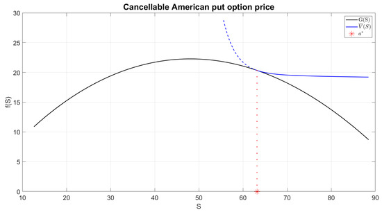
Figure 2.
Smooth fit of the payoff and the price functions for: , , , , , . denotes the value function f where or .
Author Contributions
These authors contributed equally to this work. All authors have read and agreed to the published version of the manuscript.
Funding
This work is partially supported by the Polish National Science Centre Grant No 2021/41/B/ HS4/00599.
Data Availability Statement
Not appliacable.
Conflicts of Interest
The authors declare no conflict of interest.
Appendix A
Appendix A.1. Proof of Lemma 1
Appendix A.2. Proof of Lemma 2
Proof.
By using the change-of-variable formula (Peskir 2007, Thm. 3.1), we have
This follows from the triangle inequality; the fact that the sum of the three last increments of (A2) is a zero-mean UI martingale (see (Jacod and Shiryaev 2003, eq. (4.34), p. 47) and (Kyprianou 2013, Thm. 3.4, p. 18 and Rem. 3.5, p. 20)); that
and
To show (A3), observe that, from Equation (23), it follows that for , function is continuous and hence bounded and, for , the function is constant. To prove (A4), note that
Furthermore,
Indeed, defining the sequence of consecutive downward passage times of a by and , and recalling that our price process has no positive jumps and therefore passes upward in a continuous way, from the Markov property of , we have
because
by (Li and Zhou 2020, Cor. 3.4).
The proof of the main assertion now follows from Doob’s optional stopping time theorem. □
Appendix B. Proof of Theorem 2
Proof.
First, we apply the change-of-variable formula to to obtain
Note that due to assumed smoothness of V at a. Furthermore, let be the sum of the last three increments of (A6). Note that is a mean-one local martingale (see (Jacod and Shiryaev 2003, eq. (4.34), p. 47)). Using (28) and (29), we can conclude that
Let be a localizing sequence for . Using the Doob’s optional stopping time theorem, we can write for any stopping time :
Now, taking the limit with n tending to infinity and applying the Lebesgue-dominated convergence theorem, we obtain:
which completes the proof. □
Appendix C. Proof of Proposition 1
Proof.
We start the proof by showing that
and
Indeed, denoting from Yamazaki (2017), we have
and from Kyprianou (2014):
To find the option price , we consider two possible scenarios: either the underlying price hits the threshold a or it drops below the threshold a by a jump. If creeps at a, then , and therefore
In the second scenario, , and the undershoot has an exponential distribution with parameter due to the lack of memory of this distribution. Thus,
Using and the above identities completes the proof. □
References
- Avram, Florin, Andreas Kyprianou, and Martijn Pistorius. 2004. Exit problems for spectrally negative Lévy processes and applications to Russian, American and Canadized options. The Annals of Applied Probability 14: 215–38. [Google Scholar] [CrossRef]
- Cont, Rama. 2001. Empirical properties of asset returns: Stylized facts and statistical issues. Quantitative Finance 1: 223–36. [Google Scholar] [CrossRef]
- Cont, Rama, and Peter Tankov. 2004. Financial Modelling with Jump Processes. Boca Raton: Chapman & Hall. [Google Scholar]
- Detemple, Jérôme. 2006. American-Style Derivatives: Valuation and Computation. Boca Raton: Chapman and Hall/CRC. [Google Scholar]
- Dumitrescu, Roxana, Marie-Claire Quenez, and Agnès Sulem. 2018. American options in an imperfect complete market with default. ESAIM: Proceedings and Surveys 64: 93–110. [Google Scholar] [CrossRef]
- Gapeev, Pavel, and Hessah Al Motairi. 2018. Perpetual American defaultable options in models with random dividends and partial information. Risks 6: 127. [Google Scholar] [CrossRef]
- Gapeev, Pavel V., and Libo Li. 2022a. Perpetual American standard and lookback options with event risk and asymmetric information. SIAM Journal on Financial Mathematics 13: 773–801. [Google Scholar] [CrossRef]
- Gapeev, Pavel V., and Libo Li. 2022b. Optimal stopping problems for maxima and minima in models with asymmetric information. Stochastics 94: 602–28. [Google Scholar] [CrossRef]
- Gapeev, Pavel V., Libo Li, and Zhuoshu Wu. 2020. Perpetual American Cancellable Standard Options in Models with Last Passage Times. Algorithms 14: 3. [Google Scholar] [CrossRef]
- Gapeev, Pavel V., and Hessah Al Motairi. 2022. Discounted optimal stopping problems in first-passage time models with random thresholds. Journal of Applied Probability 59: 714–33. [Google Scholar] [CrossRef]
- Gapeev, Pavel V., and Neofytos Rodosthenous. 2014. Optimal stopping problems in diffusion-type models with running maxima and drawdowns. Journal of Applied Probability 51: 799–817. [Google Scholar] [CrossRef]
- Ivanovs, Jevgenijs. 2021. On scale functions for Lévy processes with negative phase–type jumps. Queueing Systems 98: 3–19. [Google Scholar] [CrossRef]
- Jacod, Jean, and Albert Shiryaev. 2003. Limit Theorems for Stochastic Processes, 2nd ed. Berlin/Heidelberg: Springer. [Google Scholar]
- Ken-Iti, Sato. 1999. Lévy Processes and Infinitely Divisible Distributions. Cambridge: Cambridge Univ. Press. [Google Scholar]
- Kuznetsov, A. E., A. Kuznetsov, and V. Rivero. 2012. The Theory of Scale Functions for Spectrally Negative Lévy Processes. In Lévy Matters II. Lecture Notes in Mathematics. Berlin/Heidelberg: Springer, vol. 2061. [Google Scholar]
- Kyprianou, Andreas E. 2013. Gerber-Shiu Risk Theory. Cham: Springer. [Google Scholar]
- Kyprianou, Andreas E. 2014. Fluctuations of Lévy Processes with Applications. Berlin/Heidelberg: Springer. [Google Scholar]
- Li, Bo, and Xiaowen Zhou. 2020. Local times for spectrally negative Lévy processes. Potential Analysis 52: 689–711. [Google Scholar] [CrossRef]
- Linetsky, Vadim. 2006. Pricing equity derivatives subject to bankruptcy. Mathematics Finance 16: 255–82. [Google Scholar] [CrossRef]
- Peskir, Goran. 2007. A Change-of-Variable Formula with Local Time on Surfaces. In Séminaire de Probabilités XL. Lecture Notes in Mathematics. Berlin/Heidelberg: Springer, vol. 1899. [Google Scholar]
- Szimayer, Alex. 2005. Valuation of American options in the presence of event risk. Finance and Stochastics 9: 89–107. [Google Scholar] [CrossRef]
- Wilmott, Paul. 2006. Paul Wilmott on Quantitative Finance. New York: John Wiley & Sons. [Google Scholar]
- Wu, Zhuoshu, and Libo Li. 2022. The American Put Option with a Random Time Horizon. arXiv arXiv:2211.13918. [Google Scholar]
- Yamazaki, Kazutoshi. 2017. Phase–Type Approximations of The Gerber–Shiu Function. Journal of the Operations Research Society of Japan 60: 337–52. [Google Scholar] [CrossRef]


Disclaimer/Publisher’s Note: The statements, opinions and data contained in all publications are solely those of the individual author(s) and contributor(s) and not of MDPI and/or the editor(s). MDPI and/or the editor(s) disclaim responsibility for any injury to people or property resulting from any ideas, methods, instructions or products referred to in the content. |
© 2023 by the authors. Licensee MDPI, Basel, Switzerland. This article is an open access article distributed under the terms and conditions of the Creative Commons Attribution (CC BY) license (https://creativecommons.org/licenses/by/4.0/).