Abstract
Considerable studies have examined the relationship between commodity markets and stock markets. This paper studies the cyclical relationship between commodity markets and stock markets with implications for investing based on index relationships. Stock markets are represented by the U.S. S&P 500 index and aggregate commodity markets by the U.S. producer price index (PPI). Tradeable market indexes readily available to investors, namely the S&P GSCI Index and the Bloomberg Commodity Index (BCOM), are also studied. An optimal bandpass filter is used to estimate the cyclical component using a pricing-performance measure of the S&P 500 relative to the PPI, based on annual data from 1871 to 2022. The S&P GSCI and the BCOM indexes are also used to test the robustness of the findings. The impacts of the financial crisis of 2008 and the coronavirus pandemic are also assessed. The overriding conclusion of the study is that a cyclical relationship exists between stock markets and commodity markets for both aggregate and tradeable indexes which can last, from peak to peak, approximately 31 years. Measuring returns and risks in a manner consistent with these cycles can shed new light on the usefulness of commodity investing via tradeable indexes in seeking efficient portfolios.
1. Introduction
Commodity markets go hand in hand with the history of mankind. In the early part of this history, commodities were used primarily as sources of human food, feed, and for rudimentary toolmaking. Access to commodity markets, either through cash transactions (spot) or futures markets (derivatives), has now become widespread, and the monetary value of commodities in financial markets today is worth trillions of dollars. Surprisingly, however, it has been only over the past two decades that investment interest in commodity markets by market observers, institutional investors, and academic researchers has increased (e.g., Bannister and Forward 2002; Beenen 2005; Rogers 2004; Fabozzi et al. 2008; Zapata et al. 2012; Rouwenhorst and Tang 2012; Bhardwaj et al. 2015; Irwin et al. 2020; Hernandez et al. 2021; Billah et al. 2023, among many others). One factor contributing to the paucity of adopting commodities in investor’s portfolios has been driven by misconceptions surrounding commodities, such as the fact that commodities are riskier than equities, there is no relationship between equity and commodity returns, and commodity risk premiums are different from those of equities (facts which the above literature has helped demystify). While many of the unique aspects of commodity markets continue to be issues of research interest, one phenomenon of a recurrent nature that has gained interest in the most recent investment literature is that of the relationship between stock and commodities prices that in the words of Prescott (1986) can be phrased as a cyclical phenomenon. Zapata et al., using an econometric model of cycles, were the first to quantify this relationship following the work of Banister and Forward using aggregated time series data. Rogers, known as a commodity investing guru in the business news media, calls commodities “hot” and “the world’s best market,” Irwin et al. find that the real-time performance of commodity futures investing has been disappointing. When considering investing in commodities, it must be noted that commodity markets have characteristics that separate them from traditional equities. First, the demand for most commodity products is inelastic (Tomek and Robinson 1991), and with a growing population, the demand for commodities continues to increase (Evans and Lewis 2005). Second, commodities are positively correlated with inflation, particularly unexpected inflation (Gorton and Rouwenhorst 2006), and as a result, commodities may serve as an inflation hedge. Third, commodities can provide equity-like returns; Bodie and Rosansky (1980), for instance, found that using commodity and stock returns from 1950–1976, the mean returns on commodity futures were similar to those of stocks. Likewise, Greer (2000), after analyzing the returns of stocks and commodities during the period 1970 to 1999, concluded that the returns in both assets were similar. Fourth, commodity price behavior is strongly linked to fluctuations in commodity-specific market fundamentals (supply, demand, biology, and natural factors) which may not affect traditional equities. These characteristics make commodities worth considering in the search for efficient portfolios.
While commodity markets are unique, their relationship to broad financial markets has gained recent interest in the finance literature, and it has been observed that their relationship tends to fluctuate with the different phases of the business cycle (Bhardwaj and Dunsby 2013). Naturally, commodity markets have exposure to natural and biological disasters, geopolitical events, financial crises, etc., that can impact the nature of their relationship to equity markets and, as such, impact the returns and risks trade-offs resulting from each asset’s price dynamics.
The purpose of this article is to investigate the historical pricing performance of commodity markets relative to traditional equities, and consistent with Zapata et al., pricing performance is used to measure the relative strength (RS) of the relationship between the S&P 500 index and an aggregate measure of commodity prices, the U.S. producer price index (PPI), over the 1871–2022 period. Unique to this article, however, is the introduction of tradeable indexes, in particular, the first major investible commodity index (the S&P GSCI), and the Bloomberg Commodity Index (BCOM)1, which have data available starting in 1960 and 1970, respectively, and that later became available to the investment community. The article further investigates the impact of two major crises, the financial crisis of 2008–2009 and the COVID-19 pandemic, on the RS relationship and historical cyclical pattern between commodity markets and the broad equity markets prior to conducting the cyclical analysis. This is carried out in order to ascertain that the cycles approach presented later in this paper does not require special modeling adaptations. It turns out that the financial crisis of 2008–2009 had a longer recessionary impact on the RS performance while the impact of the COVID-19 pandemic on the RS measure was more transitory. However, both impacts did not appreciably change the long-term trend in the RS but it took much longer to return to the trend after the financial crisis. The identified cyclical pattern that emerges is used to further measure returns and risks to commodity investing in long-investment horizons that are consistent with the RS pattern. The article focuses strictly on commodity markets using two tradeable commodity indexes, one of which is the BCOM, is based on futures markets. The overriding conclusion of our research is that the cyclical relationship between commodities and traditional equities remains very strong, lasting approximately 31 years from peak to peak, in consistency with published research. Unique to this article is the conclusion that the aggregate relationship between commodities and equities is maintained at a much lower level of disaggregation using tradeable indexes that have been available to investors for the past several decades. The finding is relevant to portfolio analysis that stocks and commodities alternate in pricing leadership in a synchronized “bulls” versus “bears” interplay that lasts almost two decades for each market.
2. Review of Literature
The cyclical phenomenon in commodity prices (agriculture-crops and livestock, industrial and precious metals, and energy) in relation to equity markets has been of increasing interest to market observers, investors, and academic researchers over the past two decades. A Web of Science (WoS) search of the literature using the keywords “commodity cycles and agriculture” and the “All Fields” option in the database, over the period January 2002 to November 2022, and conducted in early December 2022, revealed an increasing growth in publications. We added the word “agriculture” to the search to ascertain the inclusion of agricultural commodities. Traditionally, studies of commodity prices and volatility have focused on metals and energy, but agricultural commodities (spot and futures markets) have been of increasing investor interest. The results generated a cross-sectional literature including energy fuels, metals, environmental sciences, and agriculture multidisciplinary. The number of publications per year has increased from 4 in 2002 to 34 by November 2022; similarly, total citations over the same period increased from 4 in 2002 to more than 1100. Selected and well-cited articles from these results are reviewed.
In addressing the inquiry of whether commodity-serving companies deserve investor capital, Bannister and Forward (2002) graphically examined the U.S. equity market index performance relative to the commodity market index and observed that stocks and commodities have alternated leadership in a regular cyclical wave averaging 18 years. They observed that when commodity prices declined, stocks rose 11.6% per year (stock leadership), but stocks increased only 3.4% per year during inflation (commodity leadership), thus lending support to the existence of a cyclical phenomenon on the relationship between equity markets and commodity returns. Banister and Forward did not build an econometric model to estimate an approximate optimal bandpass filter for the relative market index performance.
Radetzki (2006) identified three major commodity booms since the second world war, namely 1950–51 (in response to the Korean world), 1973–74 (intensified by harvest failures and high energy costs), and 2004–onwards (which coincided with the explosive growth in China and India and their demand for raw materials). Radetzki’s results highlight that not all commodities responded with the same intensity during these three boom periods. It was found that the second boom was the most powerful in aggregate terms and was driven by the strong increase in energy prices in 1973 and 1974. Similarly, agricultural raw material prices dominated during the first boom while metals and mineral prices had the sharpest increase in the third boom. Radetzki did not attempt to discuss the implications of booms in commodity markets relative to equity markets as in Banister and Forward. However, it is noted from illustrations in Banister and Forward that the performance of stocks was superior to that of commodities from 1950 to the late 1960s, with leadership returning to commodities during the 1970s and early 1980s. Radetzki asserted that demand shocks tend to trigger commodity booms, and increases in global growth in GDP and industrial production preceded or marked the beginning of the three commodity booms. How commodity markets respond to macroeconomic performance differs from responses in traditional equity markets, and such responses can drive equity and commodity market prices in waves that last several years; this suggests that the use of the relative-strength performance measure of equity market prices to commodity market prices is a reasonable indicator of when returns in one market lead the other. An important consideration in the above two studies is that good economic performance does not always results in booming commodity market prices. Other factors unique to commodity markets such as tight production capacity and relatively small inventories emerge after long periods of low commodity prices which discourage investments in capacity expansion.
Beenen (2005) points out that institutional investor interest in commodities reflects powerful cyclical and structural forces benefiting commodity markets but also reflecting the deterioration of equity and fixed income returns of the time (compared to the 1990s). To satisfy growing investor demand, Deutsche Bank developed an Investor Guide to Commodities that put commodities into a distinct asset class, and as Rogers (2004) stated the bull market in commodities that was underway which was noted to last about 30 years or so. The guide also tried to dispel the myth about commodities that, for most people, commodities imply an elevated level of risk; yet investing in commodities does imply risks that may differ from the risk of investing in stocks and bonds, and that at certain times in the business cycle commodities have been a much better investment than most alternatives.
One of the first analyses on the returns to investing in commodity futures when compared to investing in stocks and bonds is Gorton and Rouwenhorst (2006). They constructed an equally weighted index of commodity futures monthly returns for July 1959 to March 2004 and found that fully-collateralized commodity futures have historically produced similar returns and Sharpe ratios as equities (this finding is consistent with that of Bodie and Rosansky (1980)’s data from 1949–1976). One finding in Gorton et al.’s analysis was that the historical risk premium of commodity futures is about equal to the risk premium of stocks and is more than double the risk premium of bonds, but also find that commodity futures returns are negatively correlated with those of equities and bonds. They emphasize that, to a large extent, the negative correlation is driven by different behavior over the business cycle and a positive correlation between commodity futures and inflation. While this paper did not have a large cross-section of commodities, it served to illustrate the portfolio diversification value of commodities relative to stocks and bonds. While the behavior over the business cycle is mentioned, no attempt was made to estimate the cycle in commodities relative to equities.
The correlation of commodities to stocks and bonds using ex-post business cycle conditions has been explored in the financial literature. Kat and Oomen (2006) reassess the correlation between commodities and stocks and bonds by arguing that commodities are fundamentally different from financial assets and that there are at least two reasons for a negative correlation. First, commodity prices are the result of current market conditions (rather than long-term prospects) and tie this to the business cycle by suggesting that commodities are likely to do best during the expansion phase and their worst during the recession phase. Second, commodities are more exposed to event shocks (e.g., supply cuts by OPEC, bad weather for crops, or strikes for mining) which can drive commodity prices up and produce positive returns for investors who are long in such commodities; the increased cost of raw materials, however, can put pressure on stocks. Using correlation coefficients and Kendall’s Tau between the daily excess returns on 27 commodity futures and the daily excess returns on the Dow Jones Industrial Average (DJIA), and using the whole period as well as different phases of the business cycle, they found that daily commodity futures returns are only weakly correlated with equity returns, little persistence in the correlation dynamics, and that the correlation with equity can vary over the different phases of the business cycles using NBER dating methodology, especially for energy and metals. Contradicting Gorton and Rouwenhorst, Kat and Oomen did not find that the diversification benefits of commodity futures tend to be larger at longer horizons. Kat and Oomen did not estimate the pricing performance of stocks and bonds relative to commodity markets using cycle methodologies but used business cycles based on NBER dating.
The factors that contribute to an increased interest in commodity markets by financial investors were studied by Domanski and Heath (2007). Commodity prices of energy, precious metals, base materials, and agriculture, measured by the Goldman Sachs commodity index (GSCI), and derivative activity, measured by the number of contracts outstanding (in millions), experienced an exponential growth in their time period of analysis January 1998–June 2006. Domanski and Heath point to the increasing presence of financial investors in commodity markets and how this trend has contributed to an increase in commodity market liquidity. With the increase in commodity prices during the study period, they observe a greater variety of financial investors and investment strategies in commodity markets, with passively managed investment and portfolio products being one of the areas of rapid growth. They document that by mid-2006, about $85 billion of funds were tracking the GSCI and the Dow Jones/AIG Index (two of the most popular commodity indexes financial investors follow). Similarly, the presence of hedge funds, which have a short-term focus, increased; for example, funds that were active in energy markets had tripled to more than 500 since the end of 2004, with an estimated $60 billion in assets under management. Other examples of financial investor interest in commodity markets included the number of exchange-traded funds (ETF), the introduction of complex trading strategies (e.g., cross-market arbitrage), managed money traders (MMTs) in oil and natural gas, and the increased volume of OTC transactions.
The first econometric investigation of the relationship between stocks and commodities, using a relative strength measure as in Banister and Forward, is found in Zapata et al. based on annual values of the S&P 500 and the U.S. producer price index (PPI) for the period 1871–2010. They provide a detailed analysis of the history of commodity markets and their relationship to economic growth in the U.S., farm policy, the value of the dollar, inflation, energy markets, farm credit, and bio-energy policy. As in this study, Zapata et al. used the CF bandpass filter by setting minimum and maximum values of periodicity consistent with observations made in previous studies (e.g., Banister and Forward) for commodities (18 and 36, respectively), and minimum and maximum values typical of business cycles (2 and 8 years). The analysis was carried out on the relationship between stocks and all commodities, stocks and farm products, stocks and food products, and stocks and metals. Defining the length of a cycle as the time it takes to move from peak to peak, it was found that stocks and commodities alternated in price leadership with cycles of length 29–32 years, an average of about 31 years, and this empirical regularity was similar in shape across the various commodity groups but somewhat changed in frequency and amplitude across them, thus lending support to the heterogeneity in commodities claimed by previous studies. Zapata et al. also estimated a risk-return model of commodities and individual stocks and found that, in consistency with the stock-commodity cycle, there are periods when investment interest moves with the cycles identified in their paper. While Zapata et al. analyzed various commodity groups (farm, food, energy, and metal markets), they did not study whether the estimated cyclical behavior was applicable to tradable commodity indexes. Nonetheless, the study of the stocks-commodity cyclical phenomenon became of interest to many other researchers (e.g., Chen et al. 2015; Wang et al. 2017; Galariotis and Karagiannis 2021; Hernandez et al. 2021; Reboredo et al. 2021; among many others).
3. Materials and Methods
A relative price strength measure (RS) is used to compare the long-run cyclical relationship between stock and agricultural-commodity prices (Bannister and Forward 2002). The RS compares the relative price performance of stocks and agricultural-commodity prices. The RS is computed by dividing a stock market index into a commodity index for the period 1871–2022. Banister and Forward proposed the use of the S&P 500 index to represent the broad market index in the U.S. and the Producer Price Index in the U.S. (PPI) to represent commodity market prices. When the RS moves up, it indicates that stock returns are outperforming commodity returns (a bull trend in stocks). When the RS is trending down, RS points to commodity returns outperforming stock returns (a bull trend in commodities). In this application, and consistent with commodity investment practice, the Bloomberg Commodity Index (BCOM) and the S&P Goldman Sachs Commodity Index (SPGSCI) are also used to measure the relationship to broad financial markets of two tradeable commodity indexes. While many other tradeable commodity indexes are presently used in commodity investing, we focus on the BCOM and SPGSCI since these indexes have annual data of sufficient length for comparison to their aggregate counterparts, which according to the literature, may have cycles that can last for several decades.
3.1. Measuring Cycles
The proposition of this paper is that certain frequency components of the pricing relationship between stock and commodity markets can be key inputs of investment policy. In this context, it is best to refer to it as a stock-commodities cycle phenomenon and define it as the recurrent fluctuations in the relationship between the two asset classes.2 The Christiano and Fitzgerald (2003) bandpass filter, referred to as CF hereafter, is used in this research due to its optimality in modeling time series data, which may or may not be stationary. The CF approximates an ideal bandpass filter for a time series xt and computes its cyclical and trend components. A comprehensive treatment of cycles is found in a special issue of the Journal of Applied Econometrics and particularly in the article by Harding and Pagan (2005). Briefly, the CF methodology considers a stochastic process xt, t = 1, 2, 3, …, T, which has an orthogonal decomposition given by:
The process has power only in frequencies belonging to an interval I1 in (−π,π) and has power only in the complement of I1 in (−π,π) with subinterval constants a and b bounded as 0 < a ≤ b ≤ π; defined this way, I1 = {(a,b) U (−b,−a)} with a = 2π/pu and b = 2π/pl. The period of oscillations (periodicities of ) falls between pl and pu, with 2 ≤ pl < pu < ∞; thus, in this decomposition, the time series can be written as in Equation (1). The filter weights are chosen to minimize a mean squared error function of and the filtered . The CF filter is a finite sample approximation to the ideal bandpass filter and is given by
where the weights of the approximation are a solution to
In this definition the CF filter is a finite data approximation to the ideal bandpass filter and minimizes the MSE in Equation (3), accommodates unit-root processes for nonstationary time series, and provides a good approximation in the case of stationary time series.3 Christiano and Fitzgerald provide a comparison of the performance of the CF filter relative to other popular filters such as the Baxter-King filter and the Hodrick-Prescott filter;4 they also make the filter available in various econometric packages (e.g., EVIEWS, STATA, RATS, R). The bounds for the CF filter in this article were set to coincide with the empirical regularity found in the literature (Bannister and Forward 2002) that stocks and commodities alternate in price leadership for an average of 18 years. Following standard practice, the estimated length of a cycle is defined as the time it takes from peak-to-peak or through-to-through, and since RS is a measure of relative pricing performance, the increasing phase of cycles is a measure of the length of time (in years) when stocks perform better than commodities and vice versa.
3.2. The Data
Annual average data of the Standard and ‘Poor’s (S&P 500) from 1871 to 2022 was calculated from the monthly observations from Shiller (2022), and the corresponding data needed for the annual PPI for all commodities was obtained from the Federal Reserve Bank of Saint Louis (FRED) and the Bureau of Labor Statistics (U.S. Bureau of Labor Statistics 2022). The impact of the 2008 financial crisis and the financial stress caused by the COVID-19 pandemic is also analyzed and changes in the relationship between stocks and commodity markets are summarized; monthly values of the PPI and S&P 500 from July/2007–June/2010 and January/2019–December/2021 were used for this purpose. The base year for the PPI used in this study is 1982 = 100.5
In addition to the PPI, the S&P 500 was compared to two other commodity indices: the Bloomberg Commodity Index (BCOMa futures-based index) from 1960–2022 and the S&P GSCI (SPGSCI a commodity index used as a benchmark for commodity investments) from 1970–2022. Data for both the BCOM and the SPGSCI were downloaded from Bloomberg. The S&P 500 was chosen as a benchmark for the aggregate stock market, which encompasses about 80% of available market capitalization (S&P Dow Jones Indices 2022). Note that except for Cocoa, all of the commodities included in the S&P GSCI index are also included in the BCOM. However, the BCOM includes many other commodities such as livestock, minerals, natural gas, and oil products.
4. Results
4.1. Impact of Financial and COVID-19 Crises
The effect of the 2008 financial crisis (left chart) and the COVID-19 pandemic (right chart) on the RS performance of stock and commodity markets is shown in Figure 1, using monthly values of the PPI and S&P 500 from July/2007–June/2010, and January/2019–December/2021. The financial crisis of 2008 started when foreclosure rates doubled in December 2007. While a number of macro-measures were adopted to stop the roller coaster that was about to unfold, one of the first decisions was U.S. President Bush’s signing of the Tax Rebate Act in February 2008. As the crisis unfolded with bank failures, bailouts by the Federal Reserve started in March 2008, and, of course, the bankruptcy of the Lehman Brothers created global panic, leading to the lowest point in the RS, the time at which the U.S. Dow Jones Industrial Average had a total decline of 53.4% (Figure 1, left chart). Naturally, all of these events altered the RS’s short-term trajectory, marking the end of the bull market in commodities and marking the start of a new period of growth in stock markets. The recovery phase from the financial crisis was much slower and less steep than what occurred during the COVID-19 Pandemic (Figure 1, right chart). In fact, both crises may be characterized by a “V” shape pattern, the major difference being the speed of recovery (i.e., recovery was faster during the Pandemic).
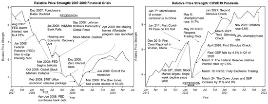
Figure 1.
Stock market (S&P 500) versus PPI for all commodities during the 2008 financial crisis and the COVID-19 pandemic.
Although the effects of the crises on unemployment and Gross Domestic Product were more severe during 2020 than during the 2008 financial crisis (Verick et al. 2022), prompt health actions and fiscal policies helped the recovery from the COVID-19 crisis at a much faster pace than that of the 2008 financial crisis (note the differences in the “V shapes”). The overriding conclusion is that the COVID-19 pandemic did not change the long-term trend of the RS between stock and commodity markets and was less impacting than the 2008 financial crisis. The extent to which the pandemic disrupted the workings of global economies, particularly the impact on supply chains, is an issue of continued analysis as of the writing of this paper. Unquestionably, however, the impact on the stability of global financial markets has been severe (e.g., Tan et al. 2022). The impacts of the coronavirus pandemic have depressed market returns for certain U.S. crop farmers and the impacts have varied depending on specific geographic areas and have worsened with the continued disputes with China. Nonetheless, ad hoc U.S. federal aid has helped support farm incomes in areas such as the U.S. Midwestern grain farms (e.g., Schnitkey et al. 2021).
4.2. Commodity Cycles
Figure 2, Figure 3 and Figure 4 show the results of the Christiano-Fitzgerald bandpass filter applied to the relative price strength (RS) of (a) stocks and the producer price index for all commodities (Figure 2), (b) stocks and the Bloomberg Commodity Index (Figure 3), and (c) and stocks and Goldman Sachs Commodity Index (Figure 4). Figure 2 shows the RS cycle over the period 1871–2022. Note that variability in the RS cycle began to increase approximately in the 1930s and continues to the present. The overall upward tendency of the RS cycle observed in Figure 2, Panel A confirms that on average, stock returns outperformed commodities over the last 151 years. However, the Christiano-Fitzgerald econometric cycle (Figure 2, Panel B) demonstrates the cyclical behavior of the relative pricing performance of stock-commodity markets. Based on Figure 2, Panel B, three cycles (from peak to peak) can be fully identified. The first cycle lasted 24 years, and the subsequent cycles had a length of 35 and 34 years, respectively. The average length of the three stock commodity cycles shown in Figure 2 is 31 years. Also, it should be noted that there is a fourth cycle in progress that began 23 years ago, whose peak is yet to occur but is quickly approaching it.
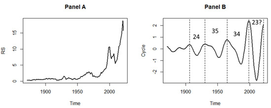
Figure 2.
Stock market (S&P 500) versus PPI for all commodities Relative Strength (Panel A) and the RS CF cycle (Panel B), Annual 1871 to 2022.
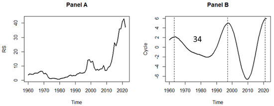
Figure 3.
Stock market (S&P 500) versus BCOM Relative Strength (Panel A) and the RS CF cycle (Panel B), Annual 1960 to 2022.
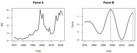
Figure 4.
Stock markets (S&P 500) versus the S&PGSCI Relative Strength (Panel A) and the RS CF cycle (Panel B), Annual 1970 to 2022.
The cyclical pattern in RS shown in Figure 2 has important implications for investors interested in commodity investing. Summary statistics tabulated from the indexes used in this article show that during the previous 151 years, the average annual returns of the S&P 500 and the PPI were 4.5% and 1.9%, respectively. But when such measures were generated by segmenting the data according to the RS cycles, it was found that when stocks outperformed commodities (uptrend phases of the RS cycle), stock annual returns were 9.25% while commodities annual returns were 0.15%. Inversely, when commodities outperform stocks (downtrend phase of the RS cycle), stock returns were −1.6%, and commodity returns were 4.9% annually. It is evident from Figure 2 that the benefit of commodity diversification may lie in their “cyclical” nature. The abundant literature promoting commodity investing generally concludes with phrases such as adding commodities provides diversification benefits during “contractions in the stock market”, which is consistent with what the RS cycle of Figure 2 reveals.
To provide a more investing-related comparison between stocks and commodities, we compared the linkage between the S&P 500 and the two investable commodity indexes, the BCOM and the S&P GSCI. Figure 3 displays the relative performance between the S&P 500 and the Bloomberg Commodity Index. The results in Figure 3, Panel B confirm that the mid-1960s to the early 1980s and during most of the decade from 2000 to 2010, were periods of high growth in commodity prices. This is consistent with historical data which show that commodity prices experienced a significant surge during the 1970s due to geopolitical events such as the oil embargo, and again in the early 2000s due to the strong demand from emerging markets such as China and India. The length of the cycle shown in Figure 3, Panel B is 34 years, which is equal to the last full cycle in Figure 2, Panel B. However, the amplitude of the cycle gets larger when BCOM is used as a proxy for commodities and is also pointing to an end in the RS expansion for stocks.
Figure 4 (Panel A) shows the price performance of the S&P 500 relative to the S&P GSCI. Launched on 11 April 1991, the S&P GSCI is a well-known benchmark for representing global commodity prices. Even though the annual index data available starting in 1970, it can be seen in Panel B that the results are very similar when using the S&P GSCI and the BCOM, which is natural given that both indices track many of the same commodities (but not the same markets).
Overall, Figure 2, Figure 3 and Figure 4 support previous literature concerning the countercyclical behavior of commodities and the stock markets. The returns in the stock market exceed the returns in the commodity markets on average. However, when investment horizons are set to the length of the RS cycle, returns from investing in indexes, such as the Bloomberg Commodity Index and the S&P Goldman Sachs Commodity Index, are higher.
5. Discussion
Applying the bandpass filter proposed by Christiano and Fitzgerald to a measure of pricing performance (RS), it is found that commodity markets, either at the aggregate level (PPI) or at the more disaggregate level (tradeable commodity indexes), follow a strong cyclical pattern with the broad market, measured by the S&P 500, that lasts about 31 years from peak to peak. This finding is consistent with the findings in previous research (e.g., Zapata et al. 2012; Bannister and Forward 2002). Naturally, the results point to alternating pricing-performance leadership over which financial markets dominate in pricing performance relative to commodities over long periods of time, and as found in other research, the length of the alternating leadership in the cycle (from peak to trough) can run for around 15 years. More specifically, the uptrend phase of the RS cycle indicates that stock returns are outperforming commodity returns. Similarly, the downtrend phase of the cycle indicates that commodity returns outperform stock returns. Data from the past 151 years provide strong evidence of four occasions on which, on average, commodities have outperformed stocks: 1907–1920, 1930–1938, 1969–1982, and 2000–2009. In essence, commodity booms happen when an unanticipated shock increases the demand for certain commodities, while the supply of those commodities takes time to determine prices. Eventually, as supply increases in response to higher prices, the cycle goes into a downturn again, which is often referred to as a “bust” (Büyükşahin et al. 2016). The rise in the price of commodities is associated with wars, inflationary periods, oil prices, and other factors that in one way or another favor the increase in prices. Certainly, the increase in the price of commodities can provide benefits for producers (e.g., farmers and metal producers) and exporting countries. However, it should not be ignored that it can also have devastating effects on those countries that depend on commodity imports and on the purchasing power of middle- or low-income consumers. From a commodity investing perspective, the cyclical interplay between stocks, as measured by the S&P 500, versus tradeable commodity indexes, merits portfolio consideration.
6. Conclusions
Since 2009, stock returns have dominated returns of commodities. However, should the cyclical phenomenon reported here continue, commodity returns will likely outperform stock returns and will continue to attract investors in the coming years. As discussed in the review of literature, wars tend to precede commodity booms. The ongoing Russian-Ukrainian war could lead to a long period of rising commodity prices. Both countries are very important players in the energy commodities, metals, and grain markets. Even if this war does not escalate to a major world conflict, its end is still uncertain, therefore a precautionary buildup of commodity inventories could trigger the next commodity price boom. Another reason for the next commodity boom could be the increasing food demand caused by a growing population. According to some estimates, the world population reached 8 billion in November 2022. This growth in the world population directly increases the demand for food commodities. A strong China recovery would also have a similar impact on commodity prices.
Whether commodity markets are “the world’s best market” (Rogers) or a market of “disappointing return” (Irwin et al. 2020) is a debate that will continue to exist. However, this article provides strong evidence that the real benefits of investing in commodities may lie in their cyclical behavior relative to stocks. Not only do commodities move over time in ups and downs in response to market fundamentals, but their cyclical behavior also tends to co-move opposite to the cycle in stocks. Therefore, an investor who follows the RS cycle can choose commodities for diversification as a hedge. To do so effectively, risk and the phase of the cycle must be accounted for. Similarly, the covariance between the two asset classes must be dynamically integrated with the cyclical relationship, a topic which is currently under investigation.
One area for future research6 on this subject is the application of econometric forecasting models to predict turning points in the RS between broad financial markets and commodity investments. Recent developments in the application of machine learning models to prediction problems in econometrics may offer paradigms for more accurate measurement of the numerous factors that impact the risk-reward relationships between stock and commodity markets and the prediction of turning points (e.g., Giusto and Piger 2017). It should also be noted that the cyclical results in this article suggest commodity leadership for the near future, and this result is consistent with the current forecast given by some market analysts. For instance, Goldman Sachs projects that the S&P GSCI, its commodities tracking index, would increase by up to 43% in 2023. The scarcity of metals and energy-related commodities would be the reason for this price spike. Stockpiles are depleting, and markets are constrained as a result of a lack of investment in mining and the search for new oil sources. Once the US and China’s economies recover from their recent economic turbulence, Goldman Sachs anticipates that the commodity market will see a boost in prices (Wallace 2022).
Thinking of commodities as heterogeneous in boom-and-bust periods implies that adding commodities to traditional portfolios of stocks and bonds must account for the difference in commodity responses to increased demand, prices, and investments. Goldman Sachs (Wallace 2022) states that underinvestment in commodity markets precedes a bullish sentiment in commodities, and that despite broadly depleted working inventories and sparse capacity nearly exhausted across most markets in commodities such as oil, capital in 2022 was not responsive to near record prices as market positioning leaned towards a recession (a point also highlighted in Banister and Forward and Radezki). Underinvestment in commodity markets, a disorderly reopening of the Chinese economy, and the rising cost of capital reduce the likelihood of sequential growth in 2023. If commodity markets remain in a state of long-run shortages with subsequent higher and more volatile prices as Goldman Sachs claims and given the recent pause in Fed rate hikes in the U.S. and the impact from the Chinese economy reopening, the leadership in commodity market returns is likely in the foreseeable future, as suggested by the estimated cycle in this paper, which at the end of 2022 is getting to close to a peak. Heterogeneity in commodity markets also implies that, for commodities such as agriculture, the response to, for instance, investments will naturally be faster than would be the case for oil and metals. In both markets, however, the nature of the response will be dictated by the cost of capital.
While the study of these research results was in progress, Goldman Sachs reaffirmed its prediction that commodity markets will be dominated by underinvestment in early 2023. The high cost of capital caused by the rise in interest rates (a deflationary action) has discouraged investors from holding commodity inventories, which could drive commodity prices higher. The cost of capital has also been linked to the withdrawal of more than $100 billion from commodity ETFs, active mutual funds, and the Bloomberg Commodity Index. What is even more worrisome according to Goldman Sachs is the underinvestment in production which leads to a reduction of commodity inventories, removing a key buffer against shocks in commodity prices. Underinvestment alone does not generate a price shock in commodity markets. Instead, it increases the sensitivity of the commodity markets to demand shocks. Cycle phenomena tend to be popular with some investors and this paper has found that using an approximation to an optimal bandpass filter, aggregate commodity market indexes (PPI) and for tradeable commodity indexes (SPGSCI and BCOM), the phenomenon repeats on average about every 31 years, in consistency with previous work on the subject (e.g., Zapata et al. 2012; Gorton and Rouwenhorst 2006). The indexes used in this study reflect the heterogeneity in commodities that tends to appeal to investors; nonetheless, the investment merits of commodities require a closer examination (e.g., Kat et al.), and preliminary work on this for global markets is beginning to emerge (e.g., Hernandez et al.). Wallace (2022) argues that an underinvestment cycle is at work in the 2023 commodity outlook. Capital expenditures and their relationship to capital consumption are drivers of the supply response in commodity markets. The relationship between these two factors and how they may contribute to the stock-commodity cyclical phenomenon in investing is an area of future research.
Author Contributions
All authors contributed equally to this work. All authors have read and agreed to the published version of the manuscript.
Funding
This research was supported in part by the USDA National Institute of Food and Agriculture, Hatch Project LAB94491, accession number 1023839.
Data Availability Statement
Data are available upon request.
Conflicts of Interest
The authors declare no conflict of interest. The funders had no role in the design of the study; in the collection, analyses, or interpretation of data; in the writing of the manuscript; or in the decision to publish the results.
Notes
| 1 | The U.S. producer price index (PPI) is a measure of the average change over time in selling prices received by domestic producers of goods and services. PPIs are available for all commodities and for various producing sectors of the U.S. economy (e.g., mining, manufacturing, agriculture, fishing, forestry) as well as natural gas, electricity, construction, etc. (https://fred.stlouisfed.org/series/PPIACO accessed on 20 November 2022). The S&P GSCI index is a benchmark for investment in the commodity markets and is a tradeable index available to market participants of the CME (it is the first major investible commodity index; the Bloomberg ticker symbol is SPGCCI—https://www.spglobal.com/spdji/en/indices/commodities/sp-gsci/#overview accessed on 20 November 2022). The Bloomberg Commodity Index (ticker symbol BCOM—https://www.bloomberg.com/ accessed on 20 November 2022) provides a broad-based exposure to physical commodities via commodity futures contracts, and no single commodity or commodity sector dominates the index. Components of all the above indexes can be found at the links provided above. |
| 2 | This view is consistent with the theory of business cycles (e.g., Prescott 1986; Lucas 1977). If we knew exactly which theoretical model best represents the economy of the U.S., then we could derive theoretical findings for cyclical behavior. As discussed in Prescott, if markets did not display this cyclical phenomenon, it would be puzzling no matter what the true model of the economy is. |
| 3 | Test of unit-roots, using the augmented Dickey-Fuller statistics with a drift, indicated that RSt has a unit-root, and therefore, the CF filter was specified with a drift and a unit-root. Cointegration tests between the S&P500 and the PPI, resulted in no cointegration for the study period 1960–2022. |
| 4 | Wavelet analysis is an alternative approach to cycle analysis. Cyclical behavior and its components can be analyzed where higher levels of precision of the wavelet approximations are constructed so that it effectively produces a band pass filter that isolates the cycle. The Christiano-Fitzgerald bandpass filter used here to isolate the cycle, which covers both stationary and nonstationary processes, is a similar procedure (e.g., Bowden and Zhu 2008). |
| 5 | We use the base 1982 = 100 because this is the measure that is most widely available in the U.S. (see https://fred.stlouisfed.org/ accessed on 20 November 2022 and search for PPI). Most research in the U.S. use this base in their work. See Tomek and Robinson (1991) for details. |
| 6 | Another potential topic of future research is the application of theories that fit long-term cycles such as Long Wave Theories. We thank an anonymous reviewer for pointing this out. |
References
- Bannister, Barry, and Paul Forward. 2002. The Inflation Cycle of 2002 to 2015. Legg Mason Equity Research, April 19. [Google Scholar]
- Beenen, Jelle. 2005. Commodities as a strategic investment for PGGM. In An Investors Guide to Commodities. London: Deutsche Bank AG London, Winchester House. [Google Scholar]
- Bhardwaj, Geetesh, and Adam Dunsby. 2013. The Business Cycle and the Correlation between Stocks and Commodities. The Journal of Investment Consulting 14: 14–25. [Google Scholar] [CrossRef]
- Bhardwaj, Geetesh, Gary Gorton, and Geert Rouwenhorst. 2015. Facts and Fantasies about Commodity Futures Ten Years Later. No. w21243. Cambridge: National Bureau of Economic Research. [Google Scholar]
- Billah, Mabruk, Faruk Balli, and Indrit Hoxha. 2023. Extreme connectedness of agri-commodities with stock markets and its determinants. Global Finance Journal 56: 100824. [Google Scholar] [CrossRef]
- Bodie, Zvi, and Victor I. Rosansky. 1980. Risk and Return in Commodity Futures. Financial Analysts Journal 36: 27–31. [Google Scholar] [CrossRef]
- Bowden, Roger, and Jennifer Zhu. 2008. The agribusiness cycle and its wavelets. Empirical Economics 34: 603–22. [Google Scholar] [CrossRef]
- Büyükşahin, B., K. Mo, and K. Zmitrowicz. 2016. Commodity Price Supercycles: What are they and What lies ahead? Bank of Canada Review-Autumn, 35–46. [Google Scholar]
- Chen, Songjiao, William W. Wilson, Ryan Larsen, and Bruce Dahl. 2015. Investing in agriculture as an asset class. Agribusiness 31: 353–71. [Google Scholar] [CrossRef]
- Christiano, Lawrence J., and Terry J. Fitzgerald. 2003. The Band Pass Filter. International Economic Review 44: 435–65. [Google Scholar] [CrossRef]
- Domanski, Dietrich, and Alexandra Heath. 2007. Financial Investors and Commodity Markets. BIS Quarterly Review, 53–67. [Google Scholar]
- Evans, Mark, and Andrew C. Lewis. 2005. Dynamics metals demand model. Resource Policy 30: 55–69. [Google Scholar] [CrossRef]
- Fabozzi, Frank J., Roland Fuss, and Dieter G. Kaiser. 2008. The Handbook of Commodity Investing. New York: John Wiley & Sons. [Google Scholar]
- Galariotis, Emilios, and Konstantinos Karagiannis. 2021. Cultural dimensions, economic policy uncertainty, and momentum investing: International evidence. The European Journal of Finance 27: 976–93. [Google Scholar] [CrossRef]
- Giusto, Andrea, and Jeremy Piger. 2017. Identifying business cycle turning points in real time with vector quantization. International Journal of Forecasting 33: 174–84. [Google Scholar] [CrossRef]
- Gorton, Gary, and K. Geert Rouwenhorst. 2006. Facts and fantasies about commodity futures. Financial Analysts Journal 62: 47–68. [Google Scholar] [CrossRef]
- Greer, Robert. 2000. The Nature of Commodity Index Returns. The Journal of Alternative Investments 3: 45–52. [Google Scholar] [CrossRef]
- Harding, Don, and Adrian Pagan. 2005. A Suggested Framework for Classifying the Models of Cycles Research. Journal of Applied Econometrics 20: 151–59. [Google Scholar] [CrossRef]
- Hernandez, Jose A., Sang H. Kang, and Seong-Min Yoon. 2021. Spillovers and portfolio optimization of agricultural commodity and global equity markets. Applied Economics 53: 1326–41. [Google Scholar] [CrossRef]
- Irwin, Scott H., Dwight R. Sanders, Aaron Smith, and Scott Main. 2020. Returns to Investing in Commodity Futures: Separating the Wheat from the Chaff. Applied Economic Perspectives and Policy 42: 583–610. [Google Scholar] [CrossRef]
- Kat, Harry M., and Roel C. A. Oomen. 2006. What every investor should know about commodities, Part II: Multivariate return analysis. Alternative Research Centre Working Paper 33. [Google Scholar] [CrossRef]
- Lucas, Robert E. 1977. Understanding business cycles. Journal of Monetary Economics 3: 7–21. [Google Scholar] [CrossRef]
- Prescott, Edward C. 1986. Theory ahead of business-cycle measurement. In Carnegie-Rochester Conference Series on Public Policy. Amsterdam: North-Holland, vol. 25, pp. 11–44. [Google Scholar]
- Radetzki, Marian. 2006. The anatomy of three commodity booms. Resources Policy 31: 56–64. [Google Scholar] [CrossRef]
- Reboredo, Juan Carlos, Andrea Ugolini, and Jose Arreola Hernandez. 2021. Dynamic spillovers and network structure among commodity, currency, and stock markets. Resources Policy 74: 102266. [Google Scholar] [CrossRef]
- Rogers, Jim. 2004. Hot Commodities: How Anyone Can Invest Profitably in the World’s Best Market. New York: John Wiley & Sons. [Google Scholar]
- Rouwenhorst, K. Geert, and Ke Tang. 2012. Commodity Investing. Annual Review of Financial Economics 4: 447–67. [Google Scholar] [CrossRef]
- S&P Dow Jones Indices. 2022. S&P 500. Available online: https://www.spglobal.com/spdji/en/indices/equity/sp-500/#overview (accessed on 20 November 2022).
- Schnitkey, Gary D., Nicholas D. Paulson, Scott H. Irwin, Jonathan Coppess, Bruce J. Sherrick, Krista J. Swanson, Carl R. Zulauf, and Todd Hubbs. 2021. Coronavirus Impacts on Midwestern Row-Crop Agriculture. Applied Economic Perspectives and Policy 43: 280–91. [Google Scholar] [CrossRef] [PubMed]
- Shiller, Robert. 2022. Available online: http://www.econ.yale.edu/~shiller/data.htm (accessed on 20 November 2022).
- Tan, Xiaoyu, Shiqun Ma, Xuetong Wang, Chao Feng, and Lijin Xiang. 2022. The impact of the COVID-19 pandemic on the global dynamic spillover of financial market risk. Frontiers in Public Health 10: 963620. [Google Scholar] [CrossRef] [PubMed]
- Tomek, William G., and Kenneth L. Robinson. 1991. Agricultural Product Prices. Ithaca: Cornell University Press. [Google Scholar]
- U.S. Bureau of Labor Statistics. 2022. Available online: stats.bls.gov (accessed on 20 November 2022).
- Verick, Sher, Dorothea Schmidt-klau, and Sangheon Lee. 2022. Is this time really different? How the impact of the COVID-19 crisis on labour markets contrasts with that of the global financial crisis of 2008–09. International Labour Review 161: 125–48. [Google Scholar] [CrossRef] [PubMed]
- Wallace, Paul. 2022. Goldman Says Commodities Will Gain 43% in 2023 as Supply Shortages Bite. Bloomberg. Available online: https://www.bloomberg.com/news/articles/2022-12-15/goldman-commodity-supercycle (accessed on 2 February 2023).
- Wang, Luo, Bin Li, Rakesh Gupta, Jen-Je Su, and Benjamin Liu. 2017. Return predictability in Australian Managed Funds. International Journal of Business Economics 16: 1–19. [Google Scholar]
- Zapata, Hector O., Joshua D. Detre, and Tatsuya Hanabuchi. 2012. Historical performance of commodity and stock markets. Journal of Agricultural and Applied Economics 44: 339–57. [Google Scholar] [CrossRef]


Disclaimer/Publisher’s Note: The statements, opinions and data contained in all publications are solely those of the individual author(s) and contributor(s) and not of MDPI and/or the editor(s). MDPI and/or the editor(s) disclaim responsibility for any injury to people or property resulting from any ideas, methods, instructions or products referred to in the content. |
© 2023 by the authors. Licensee MDPI, Basel, Switzerland. This article is an open access article distributed under the terms and conditions of the Creative Commons Attribution (CC BY) license (https://creativecommons.org/licenses/by/4.0/).