Abstract
This paper examines the performance of actively managed portfolios constructed using target price recommendations provided by analysts. We propose two methods for constructing portfolios based on Bloomberg’s 12-month target price consensus, which serves as a signal to buy or sell assets. Using a sample of 50 European stocks over a 19-year period (from 1 April 2004 to 31 March 2023), we compare the performance of target-price-based portfolios to traditional alternatives, such as a naïve homogeneous portfolio and the Eurostoxx 50 index, as well as to passive portfolios based on average recommendations. We also look into the mean-variance efficiency of these portfolios and find that all exhibit similar levels of efficiency, which are well below the performance of the theoretical tangent portfolios. Our results indicate that target-price-based portfolios show performance very close to that of the naïve homogeneous portfolio. Even the passive “average” target price portfolios, which require previous knowledge of targets for the entire investment period, are unable to outperform the naïve portfolio. Our main findings are based on a 15-year investment horizon but are robust when considering smaller maturities and out-of-sample data. We also investigate the impact of rebalancing on portfolio performance and find that it does pay off in the long run (over an 8-year investment period), but the frequency of rebalancing matters. Rebalancing only once a year is as detrimental to performance as not rebalancing at all. However, it is unclear whether the transaction costs associated with frequent rebalancing would offset any relative outperformance. Overall, our study contributes to the literature on portfolio management and market efficiency by demonstrating the potential benefits and limitations of using target price recommendations to construct portfolios, highlighting the importance of carefully considering rebalancing strategies to achieve optimal performance.
JEL Classification:
G11; G02
1. Introduction
Currently, millions of shares are traded daily on global markets, and investors often wonder if they are buying or selling at fair prices. Supporters of market efficiency argue that market prices are inherently fair and that there is no added value to stock picking (e.g., Fama 1970).
However, financial markets are flooded with financial analysts who continuously analyse stocks and provide buy/hold/sell recommendations, suggesting that it is possible to “beat” the market by following their advice. These analyses often include “price targets”. As Bilinski et al. (2013) explains, “a target price forecast reflects the analyst’s estimate of the firm’s stock price level in 12 months, providing easy-to-interpret, direct investment advice”. Target prices are typically determined based on various factors, such as the company’s financial performance, market trends, and overall economic conditions. Analysts may use different valuation techniques, such as discounted cash flow analysis, price-to-earnings ratios, and other financial metrics, to arrive at a target price for a security.
Nowadays, price targets provided by financial analysts are readily available to investors through platforms like Bloomberg or Yahoo Finance and can be used to formulate investment strategies. While price targets may vary across analysts due to the models they use and parameter estimations, general statistics provided by financial data platforms can still be relied upon.
In recent years, the use of price targets has become increasingly prevalent in the financial industry, with many analysts using these targets to provide investment recommendations (Bahaji 2021) or to establish connections to other important variables such as environmental sustainability and governance (ESG) scores (Bolognesi and Burchi 2023; Cheng et al. 2019).
Other studies have focused on the impact of the recent European regulations (such as MiFID II) on the accuracy of target prices. The authors of Fang et al. (2020) concluded that while the number of analysts has decreased with the new regulations, the quality of research and accuracy of target prices has increased.
Furthermore, the availability of price targets has been made easier by technological advancements in recent years. We highlight how the increased availability of big data and machine learning has enabled the development of algorithms that can automatically generate price targets for stocks.
Despite the increasing use of price targets, it is important to note that these targets are far from infallible, and investors should use them in combination with other factors when making investment decisions. In fact, some studies have suggested that price targets can be subject to biases, such as first impression bias (Hirshleifer et al. 2021), diagnostic bias (Bordalo et al. 2019), or herding behaviour among analysts (Gu et al. 2022), but there seems to also be evidence that investors may be able to appropriately discount those biases (Baird 2020).
Overall, the use of price targets by financial analysts has become a common practice in the industry and has been facilitated by technological advancements in recent years. While price targets can be a useful tool for investors, it is important to be aware of their limitations and use them in conjunction with other factors when making investment decisions.
In this study, we utilize Bloomberg’s 12-month consensus target prices for 50 of the most highly capitalised European stocks over the past 15 years and explore how they can be used to construct active portfolios. This issue has been largely overlooked in the literature, with Barber et al. (2001) being an exception, as the authors focused on the profitability of investment strategies based on recommendation ratings instead of target prices.
To the best of our knowledge, our study is the first to consider a large number of European stocks and directly incorporate target prices in portfolio construction. We propose ways to use the resulting price spreads (difference between the current price and the target price) in the construction of active portfolios and test the relative performance of such portfolios.
Our focus is on long-term investments of 15 years, and we also examine the importance of different rebalancing schemes. The results of rebalancing schemes are also novel in the literature on European stocks. Additionally, we test the robustness of our findings by considering alternative investment periods ranging from as short as 1 month to as long as 10 years. For a given investment period, we consider all possible maturities in our sample. The results, although challenging to visualize due to the number of portfolios per maturity and strategy, support our 15-year findings.
Furthermore, we conduct an out-of-sample analysis using the most recent data, from 1 April 2020 to 31 March 2023, which include the COVID-19 pandemic and the Ukraine war periods. Despite this, the performance results remain consistent.
The rest of the text is organized as follows. Section 2 provides a literature review and discusses the contribution of our study. Section 3 presents the data and methodology used. In Section 4, we present and discuss the results. Finally, Section 5 summarizes the main findings and presents potential avenues for future research.
2. Literature Review
The debate on whether price targets can be used to “beat” the market is closely related to the ongoing discussion about passive versus active portfolio management, as well as the broader topic of market efficiency. Several studies, such as Fama (1965), Fama et al. (1969), Barr Rosenberg and Lanstein (1984), Sharpe (1991), Admati and Pfleiderer (1997), Sorensen et al. (1998), Malkiel (2003), Shukla (2004), French (2008), Vermorken et al. (2013), Cao et al. (2017), and Elton et al. (2019), have explored this issue over time.
While the literature on market efficiency presents mixed evidence depending on specific markets, asset classes, and forms of efficiency being analysed (see, for instance, Dimson and Mussavian (1998) for an overview), there seems to be a general consensus that, particularly for large-capitalisation stocks, markets are expected to be at least semi-efficient. In other words, it is generally believed that one should not be able to trade profitably based on publicly available information, such as analysts’ recommendations and target prices. However, research departments of brokerage houses continue to spend significant sums of money on security analysis, especially for large capitalisation stocks, presumably because they believe it can generate superior returns (Barber et al. 2001), suggesting that markets may not be as efficient as previously thought.
In addition to the argument of market inefficiency, target prices may also act as self-fulfilling prophecies in financial markets. This concept has been discussed in earlier works, such as Krishna (1971) and more recent overviews, like Zulaika (2007). A self-fulfilling prophecy refers to an event that occurs because of the preceding prediction or expectation of its occurrence. When a large number of traders base their decisions on the same indicators, using the same information to take positions and push prices in the predicted direction, it can create a self-fulfilling prophecy. This argument has been commonly used in studies on financial bubbles (Garber 1989), market cycles (Farmer Roger 1999), and panics (Calomiris and Mason 1997) and has also been used to justify certain trading practices, such as technical analysis (Menkhoff 1997; Oberlechner 2001; Reitz 2006) and momentum trading (Jordan 2014). It is worth noting that most analysts who determine price targets work at high-status entities such as consulting firms and investment banks, and the reputation of these entities can significantly influence investor behaviour, supporting the argument of self-fulfilling prophecies. For more on target price accuracy, we refer to Almeida and Gaspar (2021) and references therein, as well as to Palley et al. (2021), who looked into the effect of dispersion in target prices rather than “consensus”.
More recently, there has been some research on the relationship between target prices and ESG scores. Cheng et al. (2019) concluded that strong corporate governance improves target price accuracy. Umar et al. (2022) evaluated the relationship between ESG scores and the target price precision of sell-side analysts. The results demonstrate that the ESG score positively impacts the target price accuracy. Bolognesi and Burchi (2023) examined whether ESG disclosure is a value driver for sell-side analysts of 3000 US-listed firms and concluded that analysts recognise a premium for firms more engaged in ESG transparency.
On the other hand, there still seems to exist evidence of bias in target prices. Hirshleifer et al. (2021) concluded that equity analysts’ forecasts, target prices, and recommendations suffer from first-impression bias; that is, if a firm performs particularly well/poorly in the year before an analyst follows it, that analyst tends to issue optimistic/pessimistic evaluations, respectively. Consistent with negativity bias, they also found that negative first impressions have a stronger effect than positive first impressions. Bahaji (2021) documented a decline in analyst opinion of the performance of most equity factors and found that their forecasts are style-biased. Dechow and You (2020) predicted optimistic bias in target prices and whether investors correctly ignore predictable bias. The results suggest that investors make similar valuation errors as analysts and/or do not perfectly back out the predicted bias in target prices. Gu et al. (2022) documented that institutional herding behaviour is associated with analyst target price revisions, with institutional investors buying the same stocks following an upward target price revision and selling it following a downward price revision.
The increasing availability of data on price targets also explains why target prices have became also a “hot topic” in the recent literature. There is an increasing number of papers based upon big data and machine learning that attempt to find their own target prices. For instance, machine learning models for stock prediction has been used to find a dominant strategy among neural networks. Cao et al. (2021) developed an AI analyst that, compared to humans, seems to generate better forecasts, especially when the firm is complex and information is high-dimensional.
Li et al. (2023) claimed that, “Analysts’ decision-making process, through which they use earnings and non-earnings forecasts to provide their target price revisions, remains opaque”, and based on decision tree analysis, they proposed a new metric to measure the extent to which extant revisions of analysts’ consensus earnings and sales forecasts are incorporated into the revisions of consensus target prices.
The perspective of this paper, however, is different from that of previously mentioned studies. Similar to Barber et al. (2001), we take a more hands-on, investor-oriented approach, but unlike them, we adopt a portfolio approach using a fixed set of assets for the entire time span under analysis1. To some extent we take the portfolio perspective of Henriksson et al. (2019), but their focus is on ESG scores instead of target prices.
The possibility of profitable short-term investment strategies based on publicly available recommendations of security analysts is suggested by the findings of Stickel (1995) and Womack (1996), who demonstrated that favourable (unfavourable) changes in individual analysts’ recommendations are accompanied by positive (negative) returns at the time of their announcement. Stickel (1995)’s primary goal was to measure the average price reaction to changes in individual analysts’ recommendations, thus taking an analyst and event-time perspective. However, in our study, we consider a long-term investment approach, although in the robustness analysis, we also examine various maturities ranging from 1 month to 15 years.
3. Data and Methodology
3.1. Data
This study focuses on 50 major European companies and on the period ranging from 1 April 2004 to 31 March 2023. Within this 19-year period, we start by excluding from the analysis the last 4 years (later used on to perform out-of-sample analysis), mainly focusing on the first 15 years.
From all the constituents of the EURO STOXX 50 index during our 15-years sample, we chose the 50 companies that stayed the longest in the index. Concretely, we look at the companies listed in Table 1. From Table 1, it is clear that we do not focus on any particular country or sector, as the listed companies belong to a variety of countries and all sorts of sectors, including air freight and logistics; airspace and defense; automobile manufactures; chemicals; construction and engineering; consumer durables and apparel; diversified chemicals; diversified banks; electric components and equipment; electric utilities; food products; food, beverage, and tobacco; healthcare equipment; industrial conglomerates; integrated oil and gas; integrated telecommunication services; movies and entertainment; multiline insurance; personal products; pharmaceuticals; real state; reinsurance; retailing; semiconductors; software; technology hardware and equipment; hypermarkets; supermarkets; convenience stores; cash and carry; and E-commerce.

Table 1.
List of European stocks under analysis (in alphabetic order).
For each of the companies under analysis, we collected weekly (close) prices and the so-called Bloomberg 12-month consensus target prices from 1 April 2004 until 31 March 2023, providing us with a total of 98,800 observations (988 observations for each variable and stock).
Although the focus of this study is portfolio performance, Figure 1 shows what would have been the evolution of opting to invest the full amount in only one of our 50 stocks2. One can also see the division between in-sample and out-of-sample periods marked with a vertical line in April 2019.
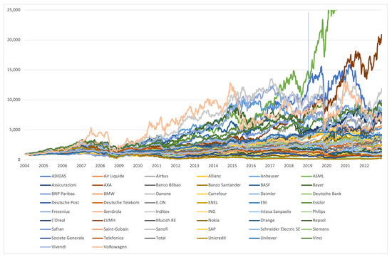
Figure 1.
Evolution of individual asset investments.
Table 2 presents some descriptive statistics on the individual stock returns for the in-sample period (first 15 years). Besides the data on individual stocks, we also collected weekly values of the EURO STOXX 50 total return index to be used as a benchmark against the portfolios under analysis.
Table 2.
Descriptive statistics of individual stock returns and Eurostoxx 50 TR.
3.2. Setup
We compare three different types of portfolios:
- Homogeneous portfolios;
- Active portfolios built based upon analysts’ recommendations;
- Mean-variance (theoretical) tangent portfolios (with and without short selling), and use the EURO STOXX 50 total return index as a benchmark.
The key idea here is to consider an initial investment of EUR 1000 and to mimic the evolution of the abovementioned portfolios during the period of 15 years, also considering a variety of possible portfolio rebalancing schemes:
- Full rebalance (which, in our case, means a weekly rebalance);
- Monthly rebalance;
- Semiannual rebalance;
- Annual rebalance; or
- No rebalance.
When rebalancing portfolios, one typically incurs costs, which may impact overall portfolio performance. These costs can arise from various sources, including transaction fees, taxes, bid–ask spreads, and other trading-related expenses. The expense ratio is the annual fee charged by a mutual fund company for managing the fund’s investments. It is expressed as a percentage of the fund’s assets under management (AUM) and covers expenses such as management fees, administrative costs, and other operational expenses but not necessarily all transaction costs. Expense ratios can range from around 0.05% to over 2%, with actively managed funds generally having higher expense ratios compared to passively managed index funds. Here, we do not take transaction costs into account when comparing the various rebalancing schemes, as our purpose is to compare strategies that have equal rebalancing dates, so all strategies would incur similar rebalancing costs.
3.2.1. Homogeneous Portfolio
Not much needs to be said about the homogeneous portfolio, (H) as, by definition, it is a portfolio assigning equal weights to all assets, also known as the portfolio. For the 50 stocks under analysis, we therefore have . Since the seminal work of DeMiguel et al. (2007), it is common practice to consider the homogeneous portfolio as minimal requirement in portfolio construction, as it is as passive and naïve as it can get.
3.2.2. Active Recommendations-Based Portfolios
There may be several ways to build portfolios based upon analysts’ recommendations. Here, we define and use the notions of absolute and relative spreads.
Let us define the absolute analysts spread of company i on date t () as the difference between the 12-month target price and the current market price:
where denotes the Bloomberg consensus target price at time t for firm i, and is the market-observed price for the same time and firm. Analysts’ spreads can be interpreted as how much, in absolute terms (say, EUR), analysts expect a particular stock to go up (for positive spreads) or to go down (for negative spreads) within the next year.
Considering a portfolio of N stocks, an investor wishing to maximize absolute gains based upon targets prices should invest in a portfolio with the following weights:
which, by definition, always add up to 1. Let us call this the absolute active portfolio (AAP). Alternatively, one could maximize relative gains by building a relative active portfolio (RAP), with the following weights:
where the relative spreads () are simply the ratio between the absolute spread and the current markets price,
Note that, by construction, we may obtain negative weights (short-selling positions) whenever target prices are below current market prices.
As spreads change constantly over time, both AAP and RAP are truly active portfolios. We call them simply (absolute or relative) “active portfolios” instead of “active recommendations-based portfolios” because the alternative portfolios in this study—homogeneous and tangent portfolios—are all passive. Figure 2 illustrates the evolution of the AAP and RAP portfolio compositions under the annual rebalancing scheme (for the full rebalancing scheme, we would have 783 different compositions).
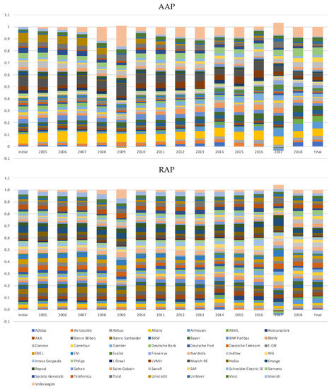
Figure 2.
Evolution of the annually rebalanced AAP portfolio.
For pure comparison purposes, we also define the mean absolute average portfolio (MAAP) and the mean relative average portfolio (MRAP). These are passive portfolios, where for each stock, we consider a fixed weight—the average weight based upon the 783 weekly weights obtained under the full rebalancing scheme.
3.2.3. Mean-Variance Tangent Portfolios
We use Markowitz (1952) mean-variance theory to determine the theoretical tangent portfolios with and without short selling, as well as the associated investment opportunity set (IOS) frontiers. These portfolios are purely theoretical, as we consider as mean-variance inputs the in-sample estimates of expected returns and the variance–covariance matrix.3 Our purpose is simply to present a view of far from the theoretical efficiency the other investments under analysis stray.
For our 15-year period, the mean-variance inputs—the vector of expected returns () and the variance–covariance matrix (V)—can be found in the first column of Table 2 or inferred from the volatilities in the third column of Table 2 and the correlation listed in Table A1 in the Appendix A. Besides the stock-related data described in Section 3.1, we also use the 15-year zero-coupon yield rate on the initial investment date (1 April 2004) as determined by the European Central Bank as the riskless rate.4 Therefore, in our computations, , which is the same value used to determine the 15-year individual investment Sharpe ratios in the last column of Table 2.
From, mean-variance theory we know the hyperbola delimiting the investment opportunity set (IOS) of all possible portfolios (w) is determined by
where , and are scalars based upon the matrix mean-variance inputs ( and V) and where is a column vector of ones. The weights of the portfolio with the maximal Sharpe ratio—the so-called tangent portfolio (T)—can then be obtained by solving the following problem:
the solution of which, in cases in which short selling is allowed, is the following well-known equation:
where represents the elements of the vector that, when short selling is not allowed, can only be solved numerically.
Here, we consider the unconstrained and constrained tangent portfolios. The weights of portfolio T in Equation (8) allow for negative (short-selling) positions and possibly Utopian extreme positions. The composition of our tangent portfolio is not as extreme as it could be.5 Still, following the common practice, we also numerically determined the portfolio with a maximal Sharpe ratio and no short selling by imposing for all i—tangent portfolio with no short selling (TNS). Figure 3 shows a mean-variance representation of all previously mentioned portfolios, including a representation of investing in individual assets.
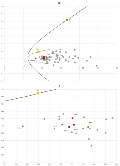
Figure 3.
Mean-variance representation. (a) Full picture. (b) Zoomed picture. Mean-variance representation of the investment opportunity set frontier assuming short selling is allowed (the hyperbola from Equation (6), blue line) or not allowed (set of constrained hyperbolas); individual assets (grey dots); the various portfolios—tangent portfolio (T, orange square), tangent portfolio with no short selling (TNS, yellow square), homogeneous portfolio (H, blue triangle), absolute and relative active portfolios (AAP and RAP; light and dark green squares, respectively), average portfolios (MAAP and MRAP; light and dark red squares, respectively), and the TR index (purple). For the active portfolios (AAP and RAP), the representation is based upon initial compositions.
Table 3 shows the actual weights determined for all portfolios. It is important to recall that the homogeneous (H), tangent (T and TNS), and mean (MAAP and MRAP) portfolios are passive, so the reported weights are those used to rebalance the portfolio on the appropriate dates for each rebalancing scheme. That is not the case for the active recommendation-based portfolios (AAP and RAP), which have different weights for all possible rebalancing dates and schemes. Having to opt for a concrete composition to use in Figure 3 and Table 3, we considered the initial compositions, which are the actual compositions over time, only for the no-rebalancing scheme. We note that the TNS portfolio requires investment in only 8 assets, which (not surprisingly) are the best-performing assets (based on the comparison of Sharpe ratios of individual assets shown in Table 2).
Table 3.
Portfolio weights.
As part of our robustness check, we also consider the alternative maturities: , , , and . For each of these maturities, we consider all possible investment start dates within the 15 years and look at the average performance of portfolios for each strategy and the EUROSTOXX TR index. This comprehensive approach allows us to thoroughly assess the effectiveness of our strategies across different investment horizons and identify any potential variations in performance based on varying time frames. Finally, we perform and out-of-sample analysis using the last 4 years of data (previously excluded from the analysis: from 1 April 2019 until 31 March 2023).
4. Results
4.1. Long-Term Investment Results
Our benchmark, the Eurostoxx 50 TR index, over the 15 years under analysis presented:
- (i)
- An annualised expected return of ;
- (ii)
- A volatility of ; and, thus,
- (iii)
- An implicit Sharpe ratio of .
Table 4 reports similar statistics for all considered portfolios and rebalancing schemes for the same 15-year investment.
Table 4.
Portfolio performance analysis.
The main conclusion seems to be that, excluding the (theoretical) tangent portfolios with a far better performance, all other portfolios present levels of performance that are comparable to the benchmark, which, itself, has a performance close to that of the homogeneous portfolio. It seems fair to say that the benchmark did not even “beat” the naïve portfolio during the 15-year period under analysis.
Looking at the performance of the portfolios that explicitly use analysts’ recommendations—AAP and RAP—they seem to perform marginally better than both the benchmark and the homogeneous portfolio using the full rebalance scheme but consistently perform worse for all other schemes. Still, the AAP portfolio performs slightly better than the RAP, possibly indicating that investors pay more attention to absolute spreads than relative spreads. However, with Sharpe ratios very close to those of the benchmark, it seems clear that these portfolios cannot “beat” the market, which points to market efficiency in the sample under analysis.
Recalling that the “mean” portfolios—MAAP and MRAP—are built based upon the observation of all recommendations over the entire 15-year period, their performance cannot be directly compared with that of the other portfolios. Still, as in the case of standard portfolios, in relative terms, we can conclude that mean absolute spreads seem to perform better than mean relative spreads (MAAP Sharpe ratios range from 0.360 to 0.365, while MRAP ratios range from 0.274 to 0.279).
Our results are robust across the various rebalancing schemes. Figure 4 reports the evolution of the various portfolios considering the two extreme rebalancing schemes: full rebalancing and no rebalancing. For all other rebalancing schemes, the evolution is “in between”. It is interesting to notice the extreme performance of the in-sample tangent portfolios (with or without short selling allowed). All other portfolios, including those based upon mean target spreads over the entire sample period, present much lower performance.
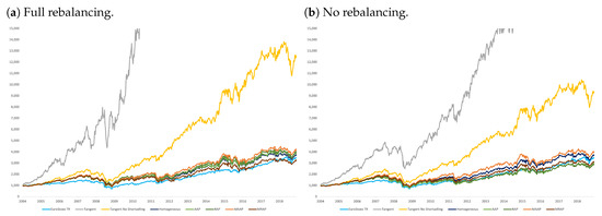
Figure 4.
Portfolio evolution.
Figure 5 compares all the rebalancing schemes for each of the trading strategies.
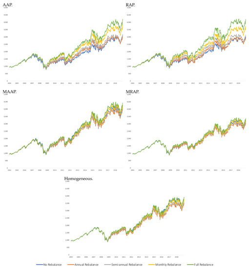
Figure 5.
Rebalancing schemes.
Looking across rebalancing schemes, both for the theoretical tangent portfolios and all other portfolios, the main conclusions are:
- Overall, performance increases with frequency of rebalancing;
- Full (i.e., weekly) rebalancing allows theoretical MVT statistics to be satisfied;
- Annual rebalancing performs as poorly as no rebalancing at all over the 15-year period; and
- The frequency of rebalancing does not seem to matter as much when each asset has a relatively small weight.
The last statement is possibly the least evident, but we note that performance seems to be rather stable across rebalancing for the passive investment schemes that assign a relatively small weight to each asset (recall Table 3), i.e., the H, MAAP, and MRAP portfolios. Figure A1 and Figure A2 in the appendix also confirm that the frequency of rebalancing matters most when the weight of individual assets is not too small. Finally, from the evolutions in Figure 5, one can conclude that rebalancing only matters after 5 or more years of investment.
4.2. Robustness Check
In our robustness analysis, we analyse the same 15-year period, but we consider various possible maturities ranging from 1 month up to 10 years and focus only on the no-rebalance cases to avoid confounding maturity effects with rebalancing. For each maturity, we consider all possible sample dates as potential start dates, except for the end of sample dates, when it would not be possible to build a portfolio with the desired maturity.
For these smaller maturities, we can consider all possible portfolios by using rolling windows of maturity size for each maturity. For example, if we consider an investment period of 1 month (), there are 765 possible portfolios with a maturity of 1 month, as our data are weekly, and there are 765 weeks in 15 years (excluding the last 4 weeks, where we can no longer invest for a full month). Likewise, we obtained 754 portfolios of semiannual maturity (), 728 of annual maturity (), 520 portfolios of 5-year maturity (), and 260 investments of 10-year maturity (). Finally, in the case of 15-year maturity, we obtained only one possible portfolio per strategy (assuming an initial investment of EUR 1000 on the first sample day and letting it run until the end.). This is the previously analysed portfolio, the results of which are repeated here for convenience.
Table 5 presents the average performance across all possible portfolios of a given maturity. Table A2 in the appendix focuses on Sharpe ratios and presents more detailed descriptive statistics. The evolution of average Sharpe ratios is also shown in Figure 6.
Table 5.
Average portfolio performance for various maturities.
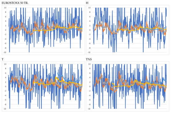
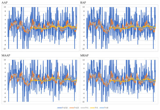
Figure 6.
Average Sharpe ratio evolution and maturity of the investment. Sharpe ratios for rolling portfolios of various maturities. Descriptive statistics of the presented ratios are presented in Table A2 in Appendix A.
One interesting observation is that volatility appears to be the most stable parameter across portfolios of different maturities, while expected returns are much more variable. For instance, extreme average expected returns, such as 76.10% for the tangent portfolio and −10.00% for the RAP portfolio, are observed for .
When looking at average Sharpe ratios (Figure 6), we note that their main feature is the incredible instability for maturities of . The significant variations in average Sharpe ratios for can be interpreted as highly unstable performance depending on which month one chooses within the 15 years under analysis, not allowing for any performance conclusion. However, for maturities of , and 10, the variations reduce significantly.
For investment strategies that depend on target prices, it is worth noting that AAP performs better for a maturity of than , which does not hold true for the other strategies. It is also remarkable to observe the relative stability of Sharpe ratios associated with the MAAP strategy.
4.3. Out-of-Sample Analysis
As mentioned earlier, we collected data spanning 19 years, allowing us to use the last 4 years for an out-of-sample analysis. Please recall Figure 1.
In this analysis, we present results not only for the out-of-sample period (1 April 2019 to 31 March 2023) but also for the full period (April 2004 to March 2023), while up to now, we had focused on the initial 15 years (1 April 2002 to 31 March 2019).
Given the coincidence of dates with the COVID pandemic, we call the first 15 years the pre-pandemic period (in-sample analysis) and the last 4 years the post-pandemic period (out-of-sample analysis), also presenting results for the full sample of 19 years.
Figure 7 highlights the in-sample and out-of-sample performance of various strategies, including H, AAP, RAP, MAAP, and MRAP. Note the vertical line on the graph separating the two periods.6 Table 6 presents the results for all portfolios.
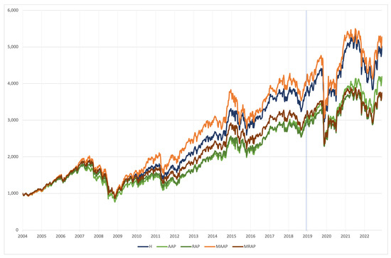
Figure 7.
Evolution of portfolios.
Table 6.
Portfolio performance analysis.
In general, the performance decreased during the out-of-sample period, both due to the non-updating of strategies and the impact of the COVID-19 pandemic and the Ukraine war. However, this decrease is particularly evident in the Sharpe ratios of the H, T, TNS, MAAP, and MRAP portfolios. Surprisingly, the active AAP and RAP portfolios did not show as significant a decrease in Sharpe ratios, with AAP showing an even higher Sharpe ratio in the post-pandemic period. Nevertheless, excluding the two tangent portfolios, T and TNS, the performance of all other portfolios for all time periods is similar to that of the homogeneous portfolio (H), attesting, once again, to market efficiency.
For completeness, we also include a full period analysis considering an investment of 19 years in all portfolios. When compared with the performance of the first 15 years (pre-pandemic period), we observed only minor changes, despite considering the no-rebalance cases. Overall, when comparing the active strategies, AAP appears to outperform all other portfolios in all periods. The passive MAAP and MRAP strategies performed considerably worse than the other portfolios in the sample, as expected, as they are based on target prices from the first 15 years.
5. Conclusions
As far as we know, this is the first study to propose concrete ways to construct active portfolios based on “consensus” target prices, which are now considered public information and can be used to make investment decisions.
We propose two active portfolios, AAP and RAP, based on absolute spreads and relative spreads, respectively. Our results show that the performance of these active strategies does not seem to “beat” that of EUROSTOXX TR or that of the naïve homogeneous portfolio, H. This is evidence of at least a semi-efficient market.
We also consider the mean-variance passive tangent portfolios, T and TNS (with and without short selling allowed) and build two passive portfolios based on the average target price recommendations, MAAP and MRAP. All these portfolios are analysed first during the period of 1 April 2004 to 31 March 2019 (15 years). It is based upon this period that we obtain the mean-variance inputs, expected returns, variances, and covariances (mean-variance inputs), as well as the average target price recommendations, so they should be interpreted as “theoretical” or “in-sample” analysis and understood in that context.
Based upon the 15 years, we are able to conclude that all portfolios based on target prices are far from efficient frontiers, even when we consider the no-short-selling (much constrained) frontier. In fact, in terms of efficiency, they do not outperform the EUROSTOXX TR or the naïve portfolio (H).
A side product of our analysis is the impact of different rebalancing schemes on the performance of portfolios. Frequency seems to matter, although not so much for the strategies based upon target prices (AAP, RAP, MAAP, and MRAP) or for the homogeneous (H) portfolio that, by construction, tends to be invested in a relatively small amount of all assets. The patterns of weight evolutions depending on rebalancing schemes in the other (mean-variance) portfolios are worth a deeper look in future studies.
Our robustness analysis focuses on the analysis of different investments within the first 15 years. Besides the long-term investment period of 15 years, we also consider all possible investments (within that 15-year period) with 1- and 6-month maturities, as well as with 1-, 5-, and 10-year maturities. The results show that the performance of all portfolios for maturities of less than a year is very unstable and that it is between the 5 to 10 years maturities that one observes a stabilisation of Sharpe ratios that converge to the performance we had in the 15 years, attesting to the robustness of our results.
The last 4 years of our sample, from 1 April 2019 to 31 March 2023, also confirms the soundness of our results, even in an out-of-sample period. Interestingly, for some of the actively managed portfolios, specifically AAP, performance increases in the out-of-sample period, while for the others, it remains stable or decreases, as one would expected, especially due to the COVID pandemic and the Ukraine war. The full sample (both in- and out-of-sample results) corroborates the idea that, at least in this market and for these particular 50 stocks, the market is at least semi-efficient. As the active portfolios proposed herein have not been studied before, future research could study their performance under other scenarios. One idea is to look into smaller-cap stocks and/or other geographical markets. However, it is worth mentioning that only for large cap firms can target prices be considered public information.
In terms of limitations, our sample period includes both the great financial crisis of 2008–2010 (in our in-sample period) and the COVID pandemic and the Ukraine war (in our out-of-sample period), which may bias the results. The sparse available literature seems to point to loss of market efficiency during the crisis periods—see, for instance, Lalwani and Meshram (2020), Gaio et al. (2022)—which we did not find. Nonetheless, it is worth recalling that this is a comparative study and that all portfolios experienced the exact same market conditions.
In addition, we focus on 50 of the largest capitalisation firms, which does not allow for extension of our results to small- and medium-capitalisation firms. The asymmetry of information between analysts and investors may be greater for smaller firms. On the other hand, “consensus” target prices on those firm may not be considered public information as are target prices of large-capitalisation firms.
It would be interesting to check if the results presented here extend to other samples in other markets and periods. Finally, it would also be interesting to determine if the relatively increased performance of more frequent rebalancing schemes is enough to cover the additional transaction costs.
Author Contributions
Conceptualization, R.M.G.; methodology, R.M.G.; software, J.A.; validation, R.M.G.; formal analysis, J.A.; investigation, J.A.; resources, J.A.; data curation, J.A.; writing—original draft preparation, J.A.; writing—review and editing, R.M.G.; visualization, R.M.G.; supervision, R.M.G.; project administration, R.M.G.; funding acquisition, R.M.G. All authors have read and agreed to the published version of the manuscript.
Funding
R.M. Gaspar is partially supported by Project CEMAPRE/REM—IODB 05069/2020 financed by the FCT/MCTES (Portuguese Science Foundation) through national funds.
Data Availability Statement
All data collected from Bloomberg.
Acknowledgments
We gratefully acknowledge the feedback from Guillermo Badia, discussant at the 12th Portuguese Finance Network Conference, as well as the meticulous reviews of the anonymous referees.
Conflicts of Interest
The authors declare no conflict of interest.
Appendix A
Table A1.
Correlation Matrix.
Table A1.
Correlation Matrix.
| Adidas | Air Liquide | Airbus | Allianz | Anheuser | ASML | Assicurazioni | AXA | B. Bilbao | B. Santander | BASF | Bayer | BNP Paribas | BMW | Danone | Carrefour | Daimler | Deutsche B. | Deutsche P. | Deutsche T. | E. ON | ENEL | ENI | Essilor | Fresenius | Iberdrola | Inditex | ING | Int. Sanpaolo | Philips | L’Oreal | LVMH | Mucich RE | Nokia | Orange | Repsol | Safran | Saint-Gobain | Sanofi | SAP | Schneider E | Siemens | Soc. Generale | Telefonica | Total | Unicredit | Unilever | Vinci | Vivendi | Volkswagen | |
| Adidas | 1.00 | |||||||||||||||||||||||||||||||||||||||||||||||||
| Air Liquide | 0.51 | 1.00 | ||||||||||||||||||||||||||||||||||||||||||||||||
| Airbus | 0.38 | 0.48 | 1.00 | |||||||||||||||||||||||||||||||||||||||||||||||
| Allianz | 0.58 | 0.64 | 0.43 | 1.00 | ||||||||||||||||||||||||||||||||||||||||||||||
| Anheuser | 0.34 | 0.40 | 0.31 | 0.37 | 1.00 | |||||||||||||||||||||||||||||||||||||||||||||
| ASML | 0.37 | 0.46 | 0.48 | 0.43 | 0.29 | 1.00 | ||||||||||||||||||||||||||||||||||||||||||||
| Assicurazioni | 0.41 | 0.54 | 0.35 | 0.63 | 0.29 | 0.37 | 1.00 | |||||||||||||||||||||||||||||||||||||||||||
| AXA | 0.54 | 0.63 | 0.45 | 0.86 | 0.32 | 0.42 | 0.70 | 1.00 | ||||||||||||||||||||||||||||||||||||||||||
| B. Bilbao | 0.45 | 0.55 | 0.39 | 0.71 | 0.33 | 0.40 | 0.71 | 0.75 | 1.00 | |||||||||||||||||||||||||||||||||||||||||
| B. Santander | 0.45 | 0.56 | 0.40 | 0.72 | 0.36 | 0.41 | 0.70 | 0.74 | 0.92 | 1.00 | ||||||||||||||||||||||||||||||||||||||||
| BASF | 0.58 | 0.74 | 0.48 | 0.75 | 0.42 | 0.48 | 0.55 | 0.69 | 0.64 | 0.63 | 1.00 | |||||||||||||||||||||||||||||||||||||||
| Bayer | 0.46 | 0.59 | 0.38 | 0.52 | 0.34 | 0.43 | 0.47 | 0.50 | 0.48 | 0.48 | 0.62 | 1.00 | ||||||||||||||||||||||||||||||||||||||
| BNP Paribas | 0.44 | 0.51 | 0.38 | 0.70 | 0.28 | 0.39 | 0.64 | 0.75 | 0.75 | 0.76 | 0.59 | 0.46 | 1.00 | |||||||||||||||||||||||||||||||||||||
| BMW | 0.55 | 0.63 | 0.48 | 0.64 | 0.39 | 0.46 | 0.49 | 0.65 | 0.56 | 0.57 | 0.73 | 0.52 | 0.57 | 1.00 | ||||||||||||||||||||||||||||||||||||
| Danone | 0.38 | 0.49 | 0.38 | 0.37 | 0.41 | 0.32 | 0.36 | 0.36 | 0.35 | 0.37 | 0.42 | 0.45 | 0.34 | 0.39 | 1.00 | |||||||||||||||||||||||||||||||||||
| Carrefour | 0.34 | 0.43 | 0.36 | 0.42 | 0.28 | 0.35 | 0.46 | 0.47 | 0.47 | 0.45 | 0.42 | 0.34 | 0.50 | 0.41 | 0.40 | 1.00 | ||||||||||||||||||||||||||||||||||
| Daimler | 0.59 | 0.65 | 0.53 | 0.70 | 0.37 | 0.50 | 0.51 | 0.68 | 0.60 | 0.59 | 0.76 | 0.53 | 0.54 | 0.82 | 0.39 | 0.43 | 1.00 | |||||||||||||||||||||||||||||||||
| Deutsche B. | 0.52 | 0.56 | 0.39 | 0.78 | 0.32 | 0.40 | 0.61 | 0.76 | 0.72 | 0.72 | 0.70 | 0.49 | 0.74 | 0.64 | 0.32 | 0.41 | 0.65 | 1.00 | ||||||||||||||||||||||||||||||||
| Deutsche P. | 0.53 | 0.59 | 0.43 | 0.68 | 0.35 | 0.41 | 0.52 | 0.65 | 0.60 | 0.59 | 0.69 | 0.52 | 0.51 | 0.61 | 0.35 | 0.37 | 0.66 | 0.61 | 1.00 | |||||||||||||||||||||||||||||||
| Deutsche T. | 0.37 | 0.47 | 0.37 | 0.48 | 0.30 | 0.36 | 0.45 | 0.43 | 0.44 | 0.45 | 0.47 | 0.47 | 0.40 | 0.41 | 0.38 | 0.38 | 0.43 | 0.42 | 0.47 | 1.00 | ||||||||||||||||||||||||||||||
| E. ON | 0.44 | 0.52 | 0.36 | 0.58 | 0.33 | 0.34 | 0.52 | 0.54 | 0.57 | 0.56 | 0.62 | 0.51 | 0.45 | 0.47 | 0.36 | 0.39 | 0.52 | 0.54 | 0.55 | 0.49 | 1.00 | |||||||||||||||||||||||||||||
| ENEL | 0.40 | 0.55 | 0.37 | 0.52 | 0.31 | 0.33 | 0.66 | 0.58 | 0.63 | 0.60 | 0.55 | 0.45 | 0.52 | 0.44 | 0.41 | 0.45 | 0.50 | 0.48 | 0.50 | 0.48 | 0.61 | 1.00 | ||||||||||||||||||||||||||||
| ENI | 0.47 | 0.61 | 0.46 | 0.57 | 0.37 | 0.42 | 0.63 | 0.59 | 0.61 | 0.60 | 0.66 | 0.55 | 0.55 | 0.55 | 0.42 | 0.46 | 0.57 | 0.55 | 0.56 | 0.46 | 0.60 | 0.63 | 1.00 | |||||||||||||||||||||||||||
| Essilor | 0.29 | 0.44 | 0.37 | 0.28 | 0.36 | 0.31 | 0.32 | 0.31 | 0.29 | 0.29 | 0.37 | 0.37 | 0.29 | 0.31 | 0.40 | 0.36 | 0.30 | 0.29 | 0.24 | 0.30 | 0.29 | 0.34 | 0.35 | 1.00 | ||||||||||||||||||||||||||
| Fresenius | 0.30 | 0.35 | 0.31 | 0.31 | 0.26 | 0.31 | 0.30 | 0.28 | 0.24 | 0.23 | 0.37 | 0.38 | 0.24 | 0.26 | 0.30 | 0.25 | 0.31 | 0.26 | 0.29 | 0.30 | 0.31 | 0.28 | 0.33 | 0.35 | 1.00 | |||||||||||||||||||||||||
| Iberdrola | 0.42 | 0.56 | 0.35 | 0.60 | 0.34 | 0.37 | 0.61 | 0.60 | 0.69 | 0.67 | 0.58 | 0.45 | 0.51 | 0.47 | 0.41 | 0.43 | 0.52 | 0.52 | 0.53 | 0.46 | 0.61 | 0.68 | 0.57 | 0.31 | 0.28 | 1.00 | ||||||||||||||||||||||||
| Inditex | 0.48 | 0.48 | 0.39 | 0.52 | 0.35 | 0.41 | 0.47 | 0.51 | 0.52 | 0.52 | 0.47 | 0.40 | 0.46 | 0.46 | 0.42 | 0.42 | 0.49 | 0.44 | 0.47 | 0.37 | 0.39 | 0.44 | 0.47 | 0.35 | 0.29 | 0.47 | 1.00 | |||||||||||||||||||||||
| ING | 0.52 | 0.60 | 0.40 | 0.79 | 0.36 | 0.39 | 0.65 | 0.82 | 0.76 | 0.74 | 0.71 | 0.51 | 0.72 | 0.61 | 0.29 | 0.42 | 0.65 | 0.75 | 0.66 | 0.38 | 0.55 | 0.57 | 0.57 | 0.30 | 0.25 | 0.59 | 0.49 | 1.00 | ||||||||||||||||||||||
| Int. Sanpaolo | 0.43 | 0.51 | 0.36 | 0.70 | 0.30 | 0.36 | 0.74 | 0.76 | 0.79 | 0.77 | 0.61 | 0.46 | 0.72 | 0.53 | 0.31 | 0.44 | 0.57 | 0.72 | 0.58 | 0.41 | 0.54 | 0.65 | 0.59 | 0.23 | 0.21 | 0.60 | 0.46 | 0.75 | 1.00 | |||||||||||||||||||||
| Philips | 0.51 | 0.58 | 0.51 | 0.64 | 0.45 | 0.57 | 0.50 | 0.63 | 0.60 | 0.58 | 0.65 | 0.55 | 0.58 | 0.59 | 0.42 | 0.44 | 0.63 | 0.60 | 0.57 | 0.46 | 0.52 | 0.48 | 0.55 | 0.35 | 0.36 | 0.50 | 0.50 | 0.64 | 0.55 | 1.00 | ||||||||||||||||||||
| L’Oreal | 0.43 | 0.58 | 0.39 | 0.48 | 0.39 | 0.42 | 0.41 | 0.46 | 0.46 | 0.44 | 0.53 | 0.49 | 0.39 | 0.46 | 0.62 | 0.45 | 0.49 | 0.40 | 0.48 | 0.45 | 0.43 | 0.47 | 0.47 | 0.42 | 0.31 | 0.50 | 0.48 | 0.41 | 0.40 | 0.52 | 1.00 | |||||||||||||||||||
| LVMH | 0.58 | 0.65 | 0.53 | 0.62 | 0.37 | 0.52 | 0.48 | 0.61 | 0.52 | 0.52 | 0.65 | 0.53 | 0.54 | 0.65 | 0.48 | 0.45 | 0.68 | 0.56 | 0.54 | 0.40 | 0.46 | 0.46 | 0.56 | 0.41 | 0.32 | 0.46 | 0.55 | 0.57 | 0.50 | 0.62 | 0.62 | 1.00 | ||||||||||||||||||
| Mucich RE | 0.48 | 0.57 | 0.41 | 0.78 | 0.34 | 0.41 | 0.60 | 0.72 | 0.60 | 0.60 | 0.65 | 0.50 | 0.60 | 0.57 | 0.37 | 0.41 | 0.61 | 0.63 | 0.56 | 0.47 | 0.50 | 0.48 | 0.54 | 0.31 | 0.32 | 0.54 | 0.47 | 0.65 | 0.58 | 0.60 | 0.46 | 0.55 | 1.00 | |||||||||||||||||
| Nokia | 0.29 | 0.34 | 0.30 | 0.39 | 0.22 | 0.38 | 0.36 | 0.40 | 0.38 | 0.39 | 0.37 | 0.34 | 0.37 | 0.39 | 0.27 | 0.31 | 0.40 | 0.36 | 0.34 | 0.29 | 0.32 | 0.33 | 0.35 | 0.16 | 0.16 | 0.39 | 0.37 | 0.38 | 0.34 | 0.38 | 0.35 | 0.39 | 0.32 | 1.00 | ||||||||||||||||
| Orange | 0.30 | 0.45 | 0.31 | 0.44 | 0.26 | 0.30 | 0.47 | 0.42 | 0.45 | 0.45 | 0.39 | 0.41 | 0.39 | 0.36 | 0.40 | 0.39 | 0.38 | 0.37 | 0.39 | 0.68 | 0.42 | 0.51 | 0.42 | 0.29 | 0.24 | 0.49 | 0.36 | 0.36 | 0.45 | 0.41 | 0.46 | 0.41 | 0.42 | 0.36 | 1.00 | |||||||||||||||
| Repsol | 0.45 | 0.58 | 0.39 | 0.59 | 0.32 | 0.40 | 0.59 | 0.59 | 0.68 | 0.69 | 0.63 | 0.50 | 0.59 | 0.55 | 0.37 | 0.40 | 0.57 | 0.55 | 0.56 | 0.43 | 0.57 | 0.54 | 0.73 | 0.28 | 0.25 | 0.62 | 0.47 | 0.57 | 0.58 | 0.52 | 0.44 | 0.53 | 0.50 | 0.38 | 0.39 | 1.00 | ||||||||||||||
| Safran | 0.43 | 0.53 | 0.59 | 0.47 | 0.26 | 0.46 | 0.38 | 0.50 | 0.42 | 0.40 | 0.53 | 0.44 | 0.42 | 0.54 | 0.36 | 0.31 | 0.57 | 0.43 | 0.47 | 0.33 | 0.36 | 0.38 | 0.46 | 0.33 | 0.34 | 0.38 | 0.41 | 0.48 | 0.38 | 0.55 | 0.45 | 0.54 | 0.44 | 0.33 | 0.28 | 0.45 | 1.00 | |||||||||||||
| Saint-Gobain | 0.57 | 0.63 | 0.53 | 0.72 | 0.33 | 0.53 | 0.59 | 0.76 | 0.66 | 0.65 | 0.71 | 0.53 | 0.67 | 0.69 | 0.42 | 0.47 | 0.74 | 0.68 | 0.64 | 0.44 | 0.50 | 0.56 | 0.59 | 0.32 | 0.28 | 0.56 | 0.54 | 0.71 | 0.66 | 0.66 | 0.51 | 0.69 | 0.62 | 0.40 | 0.42 | 0.56 | 0.55 | 1.00 | ||||||||||||
| Sanofi | 0.27 | 0.45 | 0.37 | 0.37 | 0.33 | 0.34 | 0.39 | 0.37 | 0.36 | 0.37 | 0.39 | 0.47 | 0.34 | 0.39 | 0.41 | 0.38 | 0.37 | 0.31 | 0.34 | 0.46 | 0.37 | 0.39 | 0.45 | 0.36 | 0.31 | 0.37 | 0.34 | 0.31 | 0.33 | 0.43 | 0.44 | 0.40 | 0.37 | 0.26 | 0.38 | 0.36 | 0.33 | 0.35 | 1.00 | |||||||||||
| SAP | 0.49 | 0.57 | 0.39 | 0.57 | 0.32 | 0.45 | 0.42 | 0.53 | 0.44 | 0.42 | 0.58 | 0.48 | 0.43 | 0.54 | 0.42 | 0.34 | 0.61 | 0.52 | 0.47 | 0.37 | 0.43 | 0.41 | 0.51 | 0.25 | 0.31 | 0.42 | 0.43 | 0.50 | 0.45 | 0.55 | 0.47 | 0.58 | 0.50 | 0.33 | 0.35 | 0.43 | 0.44 | 0.58 | 0.34 | 1.00 | ||||||||||
| Schneider E | 0.53 | 0.67 | 0.52 | 0.64 | 0.36 | 0.48 | 0.56 | 0.66 | 0.60 | 0.59 | 0.69 | 0.52 | 0.60 | 0.65 | 0.45 | 0.46 | 0.69 | 0.59 | 0.58 | 0.40 | 0.47 | 0.54 | 0.58 | 0.36 | 0.32 | 0.52 | 0.56 | 0.64 | 0.57 | 0.64 | 0.53 | 0.68 | 0.57 | 0.39 | 0.38 | 0.58 | 0.56 | 0.76 | 0.37 | 0.57 | 1.00 | |||||||||
| Siemens | 0.58 | 0.65 | 0.49 | 0.73 | 0.35 | 0.51 | 0.54 | 0.68 | 0.63 | 0.61 | 0.76 | 0.55 | 0.55 | 0.67 | 0.41 | 0.40 | 0.72 | 0.67 | 0.67 | 0.47 | 0.58 | 0.53 | 0.61 | 0.29 | 0.35 | 0.57 | 0.52 | 0.65 | 0.59 | 0.69 | 0.52 | 0.68 | 0.61 | 0.40 | 0.42 | 0.59 | 0.54 | 0.73 | 0.37 | 0.61 | 0.68 | 1.00 | ||||||||
| Soc.Generale | 0.45 | 0.48 | 0.34 | 0.72 | 0.36 | 0.36 | 0.66 | 0.76 | 0.76 | 0.76 | 0.60 | 0.43 | 0.83 | 0.55 | 0.28 | 0.45 | 0.55 | 0.75 | 0.55 | 0.40 | 0.51 | 0.53 | 0.55 | 0.27 | 0.22 | 0.56 | 0.46 | 0.77 | 0.76 | 0.59 | 0.35 | 0.50 | 0.62 | 0.34 | 0.38 | 0.56 | 0.36 | 0.64 | 0.32 | 0.41 | 0.56 | 0.57 | 1.00 | |||||||
| Telefonica | 0.40 | 0.58 | 0.38 | 0.60 | 0.34 | 0.37 | 0.62 | 0.58 | 0.69 | 0.71 | 0.55 | 0.50 | 0.54 | 0.50 | 0.43 | 0.43 | 0.52 | 0.54 | 0.53 | 0.59 | 0.54 | 0.58 | 0.58 | 0.32 | 0.28 | 0.67 | 0.49 | 0.53 | 0.59 | 0.50 | 0.49 | 0.49 | 0.56 | 0.36 | 0.67 | 0.65 | 0.37 | 0.55 | 0.38 | 0.44 | 0.51 | 0.55 | 0.54 | 1.00 | ||||||
| Total | 0.47 | 0.66 | 0.47 | 0.55 | 0.36 | 0.44 | 0.56 | 0.56 | 0.58 | 0.58 | 0.67 | 0.57 | 0.55 | 0.56 | 0.46 | 0.46 | 0.58 | 0.54 | 0.54 | 0.47 | 0.58 | 0.59 | 0.86 | 0.38 | 0.33 | 0.55 | 0.44 | 0.52 | 0.53 | 0.56 | 0.51 | 0.60 | 0.52 | 0.36 | 0.44 | 0.73 | 0.45 | 0.59 | 0.46 | 0.51 | 0.61 | 0.63 | 0.52 | 0.57 | 1.00 | |||||
| Unicredit | 0.40 | 0.48 | 0.35 | 0.63 | 0.23 | 0.31 | 0.68 | 0.72 | 0.75 | 0.73 | 0.56 | 0.44 | 0.71 | 0.50 | 0.26 | 0.42 | 0.53 | 0.70 | 0.53 | 0.37 | 0.47 | 0.59 | 0.55 | 0.24 | 0.19 | 0.53 | 0.40 | 0.75 | 0.82 | 0.52 | 0.35 | 0.44 | 0.51 | 0.32 | 0.39 | 0.51 | 0.39 | 0.62 | 0.26 | 0.39 | 0.52 | 0.54 | 0.74 | 0.54 | 0.48 | 1.00 | ||||
| Unilever | 0.41 | 0.50 | 0.35 | 0.37 | 0.42 | 0.36 | 0.36 | 0.35 | 0.37 | 0.37 | 0.43 | 0.43 | 0.30 | 0.37 | 0.64 | 0.38 | 0.38 | 0.31 | 0.38 | 0.41 | 0.40 | 0.40 | 0.46 | 0.37 | 0.30 | 0.39 | 0.41 | 0.32 | 0.30 | 0.46 | 0.62 | 0.47 | 0.37 | 0.26 | 0.38 | 0.40 | 0.39 | 0.36 | 0.50 | 0.39 | 0.39 | 0.40 | 0.27 | 0.43 | 0.46 | 0.26 | 1.00 | |||
| Vinci | 0.54 | 0.62 | 0.47 | 0.63 | 0.30 | 0.44 | 0.55 | 0.66 | 0.61 | 0.57 | 0.65 | 0.46 | 0.57 | 0.59 | 0.39 | 0.45 | 0.67 | 0.58 | 0.58 | 0.42 | 0.51 | 0.60 | 0.59 | 0.33 | 0.29 | 0.58 | 0.51 | 0.61 | 0.60 | 0.58 | 0.49 | 0.63 | 0.54 | 0.39 | 0.44 | 0.53 | 0.50 | 0.76 | 0.33 | 0.53 | 0.69 | 0.65 | 0.55 | 0.52 | 0.59 | 0.55 | 0.37 | 1.00 | ||
| Vivendi | 0.40 | 0.55 | 0.42 | 0.55 | 0.25 | 0.41 | 0.54 | 0.56 | 0.53 | 0.52 | 0.52 | 0.47 | 0.49 | 0.46 | 0.41 | 0.42 | 0.51 | 0.49 | 0.48 | 0.48 | 0.47 | 0.53 | 0.51 | 0.32 | 0.31 | 0.50 | 0.44 | 0.49 | 0.51 | 0.53 | 0.48 | 0.52 | 0.51 | 0.33 | 0.51 | 0.46 | 0.44 | 0.57 | 0.44 | 0.44 | 0.55 | 0.55 | 0.47 | 0.55 | 0.51 | 0.46 | 0.42 | 0.57 | 1.00 | |
| Volkswagen | 0.36 | 0.38 | 0.30 | 0.41 | 0.25 | 0.35 | 0.38 | 0.42 | 0.39 | 0.39 | 0.46 | 0.37 | 0.38 | 0.56 | 0.30 | 0.29 | 0.54 | 0.40 | 0.40 | 0.27 | 0.32 | 0.33 | 0.36 | 0.18 | 0.20 | 0.35 | 0.38 | 0.40 | 0.38 | 0.40 | 0.37 | 0.47 | 0.36 | 0.32 | 0.25 | 0.41 | 0.39 | 0.44 | 0.23 | 0.38 | 0.48 | 0.44 | 0.38 | 0.36 | 0.34 | 0.37 | 0.26 | 0.41 | 0.35 | 1.00 |


Figure A1.
Portfolio weight evolution: no rebalance versus annual rebalance. Actual evolution of weights when no rebalance (left) or annual rebalance (right) is considered for the following portfolios: H, T, TNS, AAP, RAP, MAAP, and MRAP. Vertical scales differ.
Figure A1.
Portfolio weight evolution: no rebalance versus annual rebalance. Actual evolution of weights when no rebalance (left) or annual rebalance (right) is considered for the following portfolios: H, T, TNS, AAP, RAP, MAAP, and MRAP. Vertical scales differ.


Figure A2.
Initial (blue) versus two final compositions, considering annual (orange) and no (grey) rebalance.
Figure A2.
Initial (blue) versus two final compositions, considering annual (orange) and no (grey) rebalance.


Table A2.
Sharpe ratio descriptive statistics for performance at various maturities.
Table A2.
Sharpe ratio descriptive statistics for performance at various maturities.
| EUROSTOXX 50 TR | |||||
| mean | 1.6064 | 0.7097 | 0.6437 | 0.5718 | 0.5095 |
| median | 1.2271 | 0.6886 | 0.6803 | 0.6888 | 0.3721 |
| stdev | 4.7350 | 1.2701 | 0.9562 | 0.6602 | 0.3956 |
| max | 42.5788 | 4.7517 | 3.7585 | 2.1800 | 2.3297 |
| min | −14.8995 | 2.3942 | −1.7315 | −0.3460 | 0.1927 |
| H | |||||
| mean | 2.3037 | 0.5691 | 0.6286 | 0.4179 | 0.4879 |
| median | 1.9183 | 0.4872 | 0.7662 | 0.3685 | 0.4165 |
| stdev | 5.7945 | 1.2889 | 1.0714 | 0.4552 | 0.2675 |
| min | −13.0625 | −2.4334 | −2.0381 | −0.3005 | 0.1897 |
| max | 32.0402 | 4.2547 | 3.5212 | 1.6804 | 1.5248 |
| T | |||||
| mean | 1.7145 | 1.2601 | 1.2812 | 1.6416 | 3.2754 |
| median | 1.2228 | 1.2026 | 1.2539 | 1.5107 | 2.8267 |
| stdev | 5.5047 | 1.5341 | 1.2816 | 0.7503 | 1.0881 |
| min | −24.5906 | −2.3929 | −1.6235 | 0.4065 | 1.9626 |
| max | 38.6049 | 5.3879 | 4.8460 | 4.4506 | 6.1233 |
| TNS | |||||
| mean | 1.7145 | 1.2601 | 1.2812 | 1.6416 | 3.2754 |
| median | 1.2228 | 1.2026 | 1.2539 | 1.5107 | 2.8267 |
| stdev | 5.5047 | 1.5341 | 1.2816 | 0.7503 | 1.0881 |
| min | −24.5906 | −2.3929 | −1.6235 | 0.4065 | 1.9626 |
| max | 38.6049 | 5.3879 | 4.8460 | 4.4506 | 6.1233 |
| AAP | |||||
| mean | 1.3808 | 0.5665 | 0.5175 | 0.2711 | −0.6518 |
| median | 0.6174 | 0.4549 | 0.5868 | 0.2637 | −0.6386 |
| stdev | 6.3920 | 1.3631 | 1.0320 | 0.4184 | 0.0345 |
| min | −23.9878 | −2.6447 | −1.9247 | −0.3945 | −0.7697 |
| max | 89.9684 | 4.2718 | 3.2011 | 1.2672 | −0.6255 |
| RAP | |||||
| mean | 1.3319 | 0.5345 | 0.4900 | 0.2386 | 0.2285 |
| median | 0.6192 | 0.4322 | 0.5269 | 0.2143 | 0.1828 |
| stdev | 5.6989 | 1.3441 | 1.0134 | 0.3858 | 0.1927 |
| min | −19.0181 | −2.7090 | −2.0087 | −0.4193 | 0.0170 |
| max | 50.7826 | 4.3822 | 3.0198 | 1.1536 | 0.9920 |
| MAAP | |||||
| mean | −0.2401 | 0.1326 | 0.6581 | 0.4196 | 0.5388 |
| median | −0.2096 | 0.1744 | 0.7877 | 0.2857 | 0.4258 |
| stdev | 0.4026 | 0.2208 | 1.0904 | 0.4272 | 0.2926 |
| min | −2.1475 | −0.5927 | −1.9422 | −0.2110 | 0.2141 |
| max | 1.6830 | 1.2722 | 3.6937 | 1.8812 | 1.5386 |
| MRAP | |||||
| mean | 1.4712 | 0.5899 | 0.5433 | 0.2821 | 0.3005 |
| median | 0.6999 | 0.4752 | 0.6021 | 0.2065 | 0.2312 |
| stdev | 5.9591 | 1.4035 | 1.0568 | 0.3902 | 0.2160 |
| min | −21.4155 | −2.6895 | −2.0042 | −0.3673 | 0.0638 |
| max | 55.4110 | 4.6969 | 3.2836 | 1.3277 | 1.1139 |
Descriptive statistics of the Sharpe ratio of all possible rolling portfolios with different maturities.
Notes
| 1 | Barber et al. (2001) considered stock strategies based on the most/least favourable consensus recommendations, which may lead to significant variations in the set of assets under consideration at different points in time. |
| 2 | The performance of ASML exceeded that of any other stock. The value of an investment of EUR 1000 in ASML would have reached a value close to EUR 60,000 around April 2020, then a pandemic fall close of to EUR 40,000 and recovering by the end of March 2023 to EUR 50,000. |
| 3 | In practice, estimations must naturally be out-of-sample, and the existence of estimation risk may lead to suboptimal solutions. For further details on estimation risk and robust estimation of mean-variance inputs, see, for instance, Best and Grauer (1991) and Fabozzi et al. (2007). |
| 4 | The ECB estimates daily zero-coupon yield curves for the Euro area. The “riskless” yield curve is determined by only “AAA-rated” Euro area central government bonds. For more information, see www.ecb.europa.eu/stats/financial_markets_and_interest_rates/euro_area_yield_curves/, accessed on 15 April 2023. |
| 5 | Table 3 shows that the tangent portfolio weights range from to . |
| 6 |
References
- Admati, Anat R., and Paul Pfleiderer. 1997. Does it all add up? benchmarks and the compensation of active portfolio managers. The Journal of Business 70: 323–50. [Google Scholar] [CrossRef]
- Almeida, Joana, and Raquel M. Gaspar. 2021. Accuracy of european stock target prices. Journal of Risk and Financial Management 14: 443. [Google Scholar] [CrossRef]
- Bahaji, Hamza. 2021. How valuable are target price forecasts to factor investing? Journal of Portfolio Management 48: 164–80. [Google Scholar] [CrossRef]
- Baird, Philip L. 2020. Do investors recognize biases in securities analysts’ forecasts? Review of Financial Economics 38: 623–34. [Google Scholar] [CrossRef]
- Barber, Brad, Reuven Lehavy, Maureen McNichols, and Brett Trueman. 2001. Can investors profit from the prophets? Security analyst recommendations and stock returns. The Journal of Finance 56: 531–63. [Google Scholar] [CrossRef]
- Barr Rosenberg, Kenneth Reid, and Ronald Lanstein. 1984. Persuasive evidence of market inefficiency. Journal of Portfolio Management 11: 9–17. [Google Scholar] [CrossRef]
- Best, Michael J., and Robert R. Grauer. 1991. On the sensitivity of mean-variance-efficient portfolios to changes in asset means: Some analytical and computational results. The Review of Financial Studies 4: 315–42. [Google Scholar] [CrossRef]
- Bilinski, Pawel, Danielle Lyssimachou, and Martin Walker. 2013. Target price accuracy: International evidence. The Accounting Review 88: 825–51. [Google Scholar] [CrossRef]
- Bolognesi, Enrica, and Alberto Burchi. 2023. The impact of the esg disclosure on sell-side analysts’ target prices: The new era post paris agreements. Research in International Business and Finance 64: 101827. [Google Scholar] [CrossRef]
- Bordalo, Pedro, Nicola Gennaioli, Rafael La Porta, and Andrei Shleifer. 2019. Diagnostic expectations and stock returns. The Journal of Finance 74: 2839–74. [Google Scholar] [CrossRef]
- Calomiris, Charles W., and Joseph R. Mason. 1997. Contagion and bank failures during the great depression: The june 1932 chicago banking panic. The American Economic Review 87: 863–83. [Google Scholar]
- Cao, Charles, Bing Liang, Andrew W. Lo, and Lubomir Petrasek. 2017. Hedge fund holdings and stock market efficiency. The Review of Asset Pricing Studies 8: 77–116. [Google Scholar] [CrossRef]
- Cao, Sean, Wei Jiang, Junbo L. Wang, and Baozhong Yang. 2021. From Man vs. Machine to Man + Machine: The Art and AI of Stock Analyses. Technical Report. Cambridge: National Bureau of Economic Research. [Google Scholar]
- Cheng, Lee-Young, Yi-Chen Su, Zhipeng Yan, and Yan Zhao. 2019. Corporate governance and target price accuracy. International Review of Financial Analysis 64: 93–101. [Google Scholar] [CrossRef]
- Dechow, Patricia M., and Haifeng You. 2020. Understanding the determinants of analyst target price implied returns. The Accounting Review 95: 125–49. [Google Scholar] [CrossRef]
- DeMiguel, Victor, Lorenzo Garlappi, and Raman Uppal. 2007. Optimal versus naive diversification: How inefficient is the 1/n portfolio strategy? The Review of Financial Studies 22: 1915–53. [Google Scholar] [CrossRef]
- Dimson, Elroy, and Massoud Mussavian. 1998. A brief history of market efficiency. European Financial Management 4: 91–103. [Google Scholar] [CrossRef]
- Elton, Edwin J., Martin J. Gruber, and Andre de Souza. 2019. Are passive funds really superior investments? an investor perspective. Financial Analysts Journal 75: 7–19. [Google Scholar] [CrossRef]
- Fabozzi, Frank J., Petter N. Kolm, Dessislava A. Pachamanova, and Sergio M. Focardi. 2007. Robust portfolio optimization. The Journal of Portfolio Management 33: 40–48. [Google Scholar] [CrossRef]
- Fama, Eugene F. 1965. The behavior of stock-market prices. The Journal of Business 38: 34–105. [Google Scholar] [CrossRef]
- Fama, Eugene F. 1970. Efficient capital markets: A review of theory and empirical work. The Journal of Finance 25: 383–417. [Google Scholar] [CrossRef]
- Fama, Eugene F., Lawrence Fisher, Michael C. Jensen, and Richard Roll. 1969. The adjustment of stock prices to new information. International Economic Review 10: 1–21. [Google Scholar]
- Fang, Bingxu, Ole-Kristian Hope, Zhongwei Huang, and Rucsandra Moldovan. 2020. The effects of mifid ii on sell-side analysts, buy-side analysts, and firms. Review of Accounting Studies 25: 855–902. [Google Scholar] [CrossRef]
- Farmer Roger, E. A. 1999. Macroeconomics of Self-fulfilling Prophecies. Cambridge: MIT Press. [Google Scholar]
- French, Kenneth R. 2008. Presidential address: The cost of active investing. The Journal of Finance 63: 1537–73. [Google Scholar] [CrossRef]
- Gaio, Luiz Eduardo, Nelson Oliveira Stefanelli, Tabajara Pimenta Júnior, Carlos Alberto Grespan Bonacim, and Rafael Confetti Gatsios. 2022. The impact of the russia-ukraine conflict on market efficiency: Evidence for the developed stock market. Finance Research Letters 50: 103302. [Google Scholar] [CrossRef]
- Garber, Peter M. 1989. Tulipmania. Journal of Political Economy 97: 535–60. [Google Scholar] [CrossRef]
- Gu, Chen, Xu Guo, and Chengping Zhang. 2022. Analyst target price revisions and institutional herding. International Review of Financial Analysis 82: 102189. [Google Scholar] [CrossRef]
- Henriksson, Roy, Joshua Livnat, Patrick Pfeifer, and Margaret Stumpp. 2019. Integrating esg in portfolio construction. The Journal of Portfolio Management 45: 67–81. [Google Scholar] [CrossRef]
- Hirshleifer, David, Ben Lourie, Thomas G Ruchti, and Phong Truong. 2021. First impression bias: Evidence from analyst forecasts. Review of Finance 25: 325–64. [Google Scholar] [CrossRef]
- Jordan, Steven J. 2014. Is momentum a self-fulfilling prophecy? Quantitative Finance 14: 737–48. [Google Scholar]
- Krishna, Daya. 1971. “The self-fulfilling prophecy” and the nature of society. American Sociological Review 36: 1104–7. [Google Scholar]
- Lalwani, Vaibhav, and Vedprakash Vasantrao Meshram. 2020. Stock market efficiency in the time of covid-19: Evidence from industry stock returns. International Journal of Accounting & Finance Review 5: 40–44. [Google Scholar]
- Li, Tao, Wenxiu Nan, and Jahangir Sultan. 2023. Internal relevance between analysts’ forecasts and target prices-informativeness and investment value. Applied Economics 55: 4890–910. [Google Scholar] [CrossRef]
- Malkiel, Burton G. 2003. Passive investment strategies and efficient markets. European Financial Management 9: 1–10. [Google Scholar] [CrossRef]
- Markowitz, Harry. 1952. Portfolio selection. The Journal of Finance 7: 77–91. [Google Scholar]
- Menkhoff, Lukas. 1997. Examining the use of technical currency analysis. International Journal of Finance & Economics 2: 307–18. [Google Scholar]
- Oberlechner, Thomas. 2001. Importance of technical and fundamental analysis in the european foreign exchange market. International Journal of Finance & Economics 6: 81–93. [Google Scholar]
- Palley, Asa, Thomas D. Steffen, and Frank Zhang. 2021. The Effect of Dispersion on the Informativeness of Analyst Target Prices. Available online: https://papers.ssrn.com/sol3/papers.cfm?abstract_id=3467800 (accessed on 7 October 2022).
- Reitz, Stefan. 2006. On the predictive content of technical analysis. The North American Journal of Economics and Finance 17: 121–37. [Google Scholar] [CrossRef]
- Sharpe, William F. 1966. Mutual fund performance. The Journal of Business 39: 119–38. [Google Scholar] [CrossRef]
- Sharpe, William F. 1991. The arithmetic of active management. Financial Analysts Journal 47: 7–9. [Google Scholar] [CrossRef]
- Shukla, Ravi. 2004. The value of active portfolio management. Journal of Economics and Business 56: 331–46. [Google Scholar] [CrossRef]
- Sorensen, Eric H., Keith L. Miller, and Vele Samak. 1998. Allocating between active and passive management. Financial Analysts Journal 54: 18–31. [Google Scholar] [CrossRef]
- Stickel, Scott E. 1995. The anatomy of the performance of buy and sell recommendations. Financial Analysts Journal 51: 25–39. [Google Scholar] [CrossRef]
- Umar, Muhammad, Nawazish Mirza, Syed Kumail Abbas Rizvi, and Bushra Naqvi. 2022. Esg scores and target price accuracy: Evidence from sell-side recommendations in brics. International Review of Financial Analysis 84: 102389. [Google Scholar] [CrossRef]
- Vermorken, Maximilian, Marc Gendebien, Alphons Vermorken, and Thomas Schröder. 2013. Skilled monkey or unlucky manager? Journal of Asset Management 14: 267–77. [Google Scholar] [CrossRef]
- Womack, Kent L. 1996. Do brokerage analysts’ recommendations have investment value? The Journal of Finance 51: 137–67. [Google Scholar] [CrossRef]
- Zulaika, Joseba. 2007. Self-fulfilling prophecy. In The Blackwell Encyclopedia of Sociology. Edited by George Ritzer and Chris Rojek. Hoboken: Wiley Online Library, pp. 1–3. [Google Scholar]


Disclaimer/Publisher’s Note: The statements, opinions and data contained in all publications are solely those of the individual author(s) and contributor(s) and not of MDPI and/or the editor(s). MDPI and/or the editor(s) disclaim responsibility for any injury to people or property resulting from any ideas, methods, instructions or products referred to in the content. |
© 2023 by the authors. Licensee MDPI, Basel, Switzerland. This article is an open access article distributed under the terms and conditions of the Creative Commons Attribution (CC BY) license (https://creativecommons.org/licenses/by/4.0/).