Tax Shields, the Weighted Average Cost of Capital, and the Appropriate Discount Rate for a Project with a Finite Useful Life

Abstract

The standard formulas for calculating the value of a firm’s tax shield and its weighted average cost of capital (WACC) use the assumption that the underlying cash flows are perpetuities. Yet, most projects will have a finite useful life. Because the perpetuity approach will overstate the value of a finite-life project’s tax shield, this factor will pressure the perpetuity-formula WACC to be less than the finite-life WACC. However, a large portion of the value of a perpetual tax shield can be attributed to interest payments during the next 5, 10, or 25 years, making it possible for the perpetuity-formula WACC to be greater than the finite-life WACC. Using a series of numerical examples, this paper shows that the finite-life WACC can be either higher or lower than the perpetuity-formula WACC depending on the project’s useful life, the required return on the unlevered project, the firm’s capital structure, the cost of debt, the marginal tax rate, and the debt repayment pattern (e.g., coupon bonds or amortizing loans). The analysis in this article helps managers better understand the potential biases introduced into the capital budgeting process when using the perpetuity-formula WACC to evaluate projects with finite useful lives.

1. Introduction

The standard textbook formulas for calculating the value of a firm’s tax shield and its weighted average cost of capital (WACC) use the assumption that the underlying cash flows are perpetuities, following Modigliani and Miller (1958, 1963). This assumption, however, will not be satisfied by any prospective project in which a firm might consider investing. As a result, a firm’s WACC—estimated using the perpetuity formula—is unlikely to be equal to the appropriate discount rate for a project with a finite useful life (Arditti 1973; Reilly and Wecker 1973; Myers 1974; Brick and Thompson 1978; Miles and Ezzell 1980; Miller 2009; Pierru 2009; Brusov et al. 2011; Filatova et al. 2022). Yet, the perpetuity-formula WACC continues to be widely used in practice (Bruner et al. 1998).

Prior studies reach differing conclusions about the direction and magnitude of the potential difference between a firm’s perpetuity-formula WACC and the appropriate discount rate for a project with a finite useful life (i.e., the finite-life WACC). Brick and Thompson (1978) claim that the finite-life WACC can be less than the perpetuity-formula WACC and that this difference can be large enough to distort a firm’s investment decision, potentially leading to underinvestment. In contrast, Brusov et al. (2011) claim that the finite-life WACC will exceed the perpetuity-formula WACC, potentially leading to overinvestment. The goal of this article is to resolve this conflict and to help managers better understand the potential biases introduced into the capital budgeting process when using the perpetuity-formula WACC to calculate the net present value (NPV) of projects with finite useful lives.1

Because the perpetuity approach will overstate the value of a finite-life project’s tax shield—holding the debt interest rate, the tax rate, and the size of the initial loan constant—this factor will pressure the perpetuity-formula WACC to be less than the finite-life WACC. However, because a large portion of the value of a perpetual tax shield can be attributed to interest payments during the next 5, 10, or 25 years, it is possible for the relative importance of a finite-life tax shield to be greater than that of a perpetual-life tax shield. For this reason, it is also possible for the perpetuity-formula WACC to be greater than the finite-life WACC.

This paper uses a series of numerical examples to illustrate the potential relations between a project’s finite-life WACC and a firm’s perpetuity-formula WACC. This exercise reveals that a project’s finite-life WACC can be either higher or lower than the firm’s perpetuity-formula WACC depending on the length of the project’s useful life, the required return on the unlevered project, the firm’s capital structure, the cost of debt, the marginal tax rate, and most important, the debt repayment pattern. If the debt cash flows mirror those of a coupon bond, the perpetuity-formula WACC can be higher or lower than the finite-life WACC. These differences tend to be modest, especially at lower equity risk premium levels. If the debt is structured as an amortizing loan, the perpetuity-formula WACC will be less than the finite-life WACC. When the equity risk premium is sizable—and the perpetuity-formula WACC is used as the discount rate in NPV calculations—these differences can be large enough to distort capital budgeting decisions, potentially leading to overinvestment.

Yet, the finite-life WACC is typically not a practical alternative to the perpetuity-formula WACC within the traditional capital budgeting framework. The finite-life WACC is a function of the estimated useful life, and the numerical value of the finite-life WACC can change noticeably in response to small changes in this useful life, especially when it is 25 years or less. For this reason, the perpetuity-formula WACC remains the best option to use as the discount rate within most capital budgeting applications. Nevertheless, managers should exercise caution—and be aware of the potential biases introduced into NPV calculations—when using the perpetuity-formula WACC to evaluate projects with finite useful lives.

This article is organized as follows. Section 2 illustrates the applications and limitations of the perpetuity-formula valuation approaches stemming from the Modigliani and Miller (1958, 1963) articles. Section 3 shows how to modify the tax shield and WACC calculations for projects (or firms) with finite useful lives. Numerical examples in this section show that the majority of a perpetual tax shield value will be realized in the foreseeable future. In addition, this section identifies the estimation challenges presented by the finite-life WACC formula. Section 4 compares finite-life and perpetuity-formula WACC estimates when the firm issues coupon bonds and when the debt is structured as amortizing loans. Section 5 presents an example illustrating how the difference between a project’s finite-life and perpetuity-formula WACC can affect the project’s estimated NPV. Section 6 discusses the results in this paper and offers conclusions.

2. The Perpetuity-Formula WACC

In theory, a firm’s WACC is the appropriate discount rate to use when evaluating projects with similar risk profiles to the firm as a whole. Within the traditional capital budgeting framework, stemming from Modigliani and Miller (1958, 1963), a prospective project’s estimated NPV will be equal to (or greater than) zero if the project offers an IRR that is equal to (or in excess of) the firm’s WACC. If a firm’s expected future cash flow is known, the firm’s WACC can be calculated as a function of that cash flow stream’s market value. For example, assume that a firm’s expected perpetual cash inflow is 10 and that the market value of the firm is 100. If so, the WACC of the firm is 10%, which is the IRR of a cash flow stream comprised of an initial cash outflow of 100 followed by a perpetual cash inflow of 10. If the initial investment in the firm was 80, then that initial investment generated a perpetual annual return of 12.5% and a positive NPV of 20. If the initial investment in the firm was 100, then that initial investment generated a perpetual annual return of 10% and an NPV of 0.

2.1. Firm Value and the Perpetuity-Formula WACC

Modigliani and Miller (1958, 1963) show that the value of a levered cash flow stream, V_L, is the sum of the value of the unlevered cash flow stream, V_U, and the value of the tax shields created by interest payments, V_TS, as shown in Equation (1).

V_L = V_U + V_TS

(1)

When the debt cash flows are a level perpetuity, and if the tax shields and interest payments have the same risk (i.e., the tax shields are discounted using the required return on debt, r_D), V_TS,∞ is the product of the marginal tax rate, τ, and the market value of the firm’s debt, D₀ (Modigliani and Miller 1963; Fernandez 2004; Cooper and Nyborg 2006; Barbi 2012; Campani 2015).2 This is Equation (2).

V_TS,∞ = τ D₀

(2)

Although a firm’s total market value can be quantified, the underlying cash flows supporting that market value cannot be observed. Thus, a firm’s WACC typically cannot be calculated as a function of the firm’s value and its expected future cash flow stream. Instead, a firm’s WACC must be estimated using formulas derived from the Modigliani and Miller (1958, 1963) articles. Modigliani and Miller (1963, footnote 16) show that a firm’s WACC_∞ can be calculated as a function of the unlevered required return on assets, r_A,U, the required return on debt, r_D, the marginal tax rate τ, and the ratio of the market value of the firm’s outstanding debt to the market value of the firm, W_D. This is Equation (3).

WACC_∞ = r_A,U (1 − τW_D)

(3)

Because r_A,U is the unlevered required return on assets, this return is unobservable for any firm that uses debt in its capital structure. Thus, Equation (3) is difficult to apply in practice. To operationalize Equation (3), Haley and Schall (1973, chp. 13) show how the right-hand side of the equation can be restated in terms of the required return on levered equity, r_E, the required return on debt, r_D, the marginal tax rate, τ, and the firm’s capital structure weights, W_D and W_E. W_E is the ratio of the market value of the equity to the market value of the firm. Assuming that the firm does not have preferred stock outstanding, W_E = 1 − W_D. The resulting formula, Equation (4), is what Myers (1974, p. 8) calls the “textbook formula” WACC.

WACC_∞ = r_DW_D (1 − τ) + r_EW_E

(4)

Because V_TS,∞ will accrue to the firm’s shareholders, r_E in Equation (4) is a weighted average of the unadjusted required return on the equity cash flows, $r_E^{*}$, and the required return on the tax shield, which is assumed to be equal to r_D (see note 2).

To illustrate Equations (1)–(4), assume that a firm (or a project) requires an initial investment in fixed assets of 100, funded by equal amounts of debt and equity (for simplicity, the working capital investment is set equal to 0). The required return on debt, $r_D,$ is 8% and the tax rate, $\tau$, is 25%. This investment will produce level, perpetual, asset, debt, and equity cash flow streams. Each year, the depreciation of the fixed assets (assumed to be equal to 5) is exactly offset by a new capital investment to maintain the productivity of the assets. Assuming that the investment will produce perpetual earnings before depreciation, interest, and taxes of 18.33,

Table 1. Three Cash Flow Measures. This table shows how to calculate a firm’s equity cash flow, its unlevered free cash flow, and its capital cash flow.

Balance Sheet (Initial)		Income Statement		Cash Flows
Working Cap.	0	EBITDA	18.33	Net Income	7
Fixed Assets	100	Depreciation	−5.00	+Depr.	5
Total Assets	100	EBIT	13.33	+/− Δ in WC	0
Debt	50	Interest (8%)	4.00	−CapEx	−5
Equity	50	EBT	9.33	Eq. Cash Flow	7
Total D + E	100	Taxes (25%)	2.33	Unlev. FCF	10 a
		Net Income	7.00	Cap. Cash Flow	11 b

^a Unlevered Free Cash Flow = 13.33(1 − 25%) = 10; ^b Capital Cash Flow = 7 + 4 = 11.

shows how to calculate the firm’s perpetual equity cash flow (=7), free cash flow (=10), and capital cash flow (=11) from the firm’s pro forma (perpetual) financial statements.

Using these assumptions, V_TS,∞ = 12.5 can be calculated using Equation (2) and V_L = 112.5 is calculated using Equation (1). Assuming that $r_E^{*}$ = 12%, the capital structure weights and r_E (which is the weighted average of $r_E^{*}$ and r_D) are calculated as follows.

$$W_D=\frac{50}{112.5}=0.4444$$

$$W_E=\frac{62.5}{112.5}=0.5556$$

$$r_E=8\%\frac{12.5}{62.5}+12\%\frac{50}{62.5}=11.2\%$$

To calculate the firm’s weighted average cost of capital, plug these numbers, along with $r_D=8\%$ and $\tau =25\%$, into Equation (4). Thus, $WAC{C}_{\infty }=8.889\%$.

The firm’s value of 112.5 can be recalculated in four different ways. When Equation (1) is used, the calculation is called the adjusted present value method. When the free cash flow of 10 is divided by $WAC{C}_{\infty }$ this is called the WACC approach (10/0.08889 = 112.5). When the equity cash flow of 7 is divided by $r_E$ and is then added to the debt value, this is called the flows-to-equity calculation (50 + 7/0.112 = 112.5). Finally, the firm’s value can also be calculated as a function of the “pre-tax” version of Equation (4). To do this, set $\tau =0$ in Equation (4) and solve for the adjusted WACC value of 9.778%. Then, divide the capital cash flow of 11 by the adjusted WACC (11/0.09778 = 112.5). This is the capital cash flows technique.3

2.2. Limitations of the Perpetuity-Formula WACC

The traditional perpetuity-formula WACC uses the assumption that a firm’s economic return and its cost of capital are constant over time. However, a firm’s competitive strengths and weaknesses are unlikely to remain unchanged over time, and the yield curve typically is not flat. Thus, while the constant return and the constant cost of capital assumptions serve to simplify the math, they introduce imprecision and ambiguity into the WACC calculation.4

Additional ambiguity is introduced into the process of calculating a firm’s WACC because Equation (4) requires analysts to estimate the firm’s before-tax cost of debt, the firm’s marginal tax rate, the firm’s cost of equity, and the firm’s market-value capital structure weights. As discussed in Bruner et al. (1998), there are multiple approaches that can be used to quantify each of these variables, and each approach relies on imprecise information. For example, if the capital asset pricing model is used to estimate the cost of equity, the analyst must estimate the risk-free rate, the equity market risk premium, and the firm’s Beta. Because of these challenges, Bruner et al. (1998, p. 27) conclude that “Best-practice companies can expect to estimate their weighted average cost of capital with an accuracy of no more than plus or minus 100 to 150 basis points”. Similarly, Welch (2021, p. 194) opines that we do not currently have the ability to estimate a firm’s cost of capital more precisely than at 1 percent intervals.

If the appropriate discount rate cannot be precisely quantified, any ensuing NPV calculation will provide only an approximation of a project’s true economic value. For example, assume that the true cost of capital for a project is 8% and that the project will produce free cash flows in the amount of a ten-year annuity of 100. If so, the project’s present value is 671.01. If a 7% discount rate is used, the calculated present value would be 702.36 (4.71% too high). If a 9% discount rate is used, the calculated present value would be 641.77 (4.36% too low). If the initial investment is 640, the estimated NPV will range from 1.77 (WACC = 9%) to 62.36 (WACC = 7%). Clearly, the process of evaluating potential projects is rife with uncertainty. This highlights the importance of the sensitivity analysis phase of the capital budgeting process; a project’s NPV should be recalculated using a range of discount rates.

Finally, the perpetuity-formula WACC employs the implicit assumption that the underlying cash flow streams are perpetuities and that the firm’s tax shield will accumulate over an infinite time horizon. These assumptions will not be satisfied by any prospective project in which a firm might consider investing. Thus, the perpetuity-formula WACC may not be equal to the appropriate discount rate for prospective projects with finite useful lives.5

3. The Finite-Life Formulas

If a firm (or a project) will have a finite useful life, the value of the tax shield created by tax deductible interest payments cannot be calculated using Equation (2), and its (exact) WACC cannot be calculated using Equations (3) or (4). This section shows how to calculate the value of a finite-life tax shield and explains how to calculate a firm’s finite-life WACC.

3.1. Finite-Life Tax Shields

If a firm’s unlevered and levered cash flow streams both have a finite useful life of N years, V_TS,N will be equal to the present value of the annual tax benefits r_DτD_n, where n = 1 to N, discounted using r_D (Barbi 2012). This is Equation (5).

$$V_{TS,N}={\sum }_{n=1}^N\frac{r_D\tau D_{n-1}}{{\left(1+r_D\right)}^n}$$

(5)

The value V_TS,N will depend on how the debt repayment schedule is structured. If the debt is structured as an amortizing loan, V_TS,N must be calculated using Equation (5). If the debt cash flows mirror those of a coupon bond, as in Brick and Thompson (1978) and Brusov et al. (2011), the value of the tax shield is the present value of a N-year annuity in the amount r_DτD₀. In this case, Equation (5) can be rewritten as Equation (6).

$$V_{TS,N}=r_D\tau D_0\frac{\left[1-{\left(1+r_D\right)}^{-N}\right]}{r_D}$$

(6)

Although firms typically do not issue perpetual bonds (i.e., consol bonds), many firms do replace maturing debt with new loans, effectively extending the life of the debt. Nevertheless, calculating the value of a firm’s debt tax shield using Equation (2), rather than Equations (5) or (6), is likely to overstate the value of the tax shield.

Table 2. The Relation Between Finite-Life and Perpetual Tax Shields. This table lists the ratio of V_TS,N to V_TS,∞ assuming that the debt is coupon bonds (Panel A) or amortizing loans (Panel B). In each panel, these ratios are listed for five debt interest rates, r_D = 2%, 4%, 6%, 8%, and 10%, and useful lives of N = 5, 10, 25, 50, and 100.

	Useful Life (Years)
rD (%)	5	10	25	50	100
Panel A: Coupon Bonds
2	0.094	0.180	0.390	0.628	0.862
4	0.178	0.324	0.625	0.859	0.980
6	0.253	0.442	0.767	0.946	0.997
8	0.319	0.537	0.854	0.979	0.999
10	0.379	0.614	0.908	0.991	0.999
Panel B: Amortizing Loans
2	0.058	0.105	0.235	0.420	0.686
4	0.113	0.199	0.423	0.685	0.922
6	0.163	0.284	0.570	0.838	0.983
8	0.211	0.361	0.683	0.919	0.997
10	0.255	0.430	0.769	0.961	0.999

compares estimates of V_TS,N using Equation (2), assuming N = ∞, to estimates using Equation (6), finite-life coupon bonds, and Equation (5), finite-life amortizing debt. In particular, the examples in Table 2 calculate the ratio of V_TS,N to V_TS,∞ assuming that the debt is coupon bonds (Panel A) or amortizing loans (Panel B). In each panel, these ratios are listed for five debt interest rates, r_D = 2%, 4%, 6%, 8%, and 10%, and useful lives of N = 5, 10, 25, 50, and 100 years. Because V_TS is a function of τ and D₀ in all three equations, the ratios are independent of these variables.

The results in Table 2 reveal that a large portion of V_TS,∞ can be attributed to the tax shields created by interest payments during the next 5, 10, or 25 years. For coupon bonds (Panel A), if r_D is 4%, the portion of the perpetual tax shield realized in the first 5, 10, and 25 years will be almost 18%, over 32%, and over 62%, respectively. If r_D is 8%, the portion of the perpetual tax shield realized in the first 5, 10, and 25 years will be almost 32%, almost 54%, and over 85%, respectively. For amortizing loans (Panel B), a smaller—but still sizeable—portion of the perpetual tax shield value can be attributed to interest payments during the first 25 years. If r_D is 4%, the portion of the perpetual tax shield realized in the first 5, 10, and 25 years will be over 11%, almost 20%, and over 42%, respectively. If r_D is 8%, the portion of the perpetual tax shield realized in the first 5, 10, and 25 years will be over 21%, over 36%, and over 68%, respectively.

To the extent that a large portion of the tax shield value is realized in the foreseeable future, it is possible for the relative importance of a finite-life tax shield to be equal to or greater than that of a perpetual-life tax shield. If so, it is conceivable for the finite-life WACC to approximate, or to even be less than, the perpetuity-formula WACC.

3.2. The Finite-Life WACC

Myers (1974) shows that the WACC for a levered firm operating in a one-period world can be calculated using Equation (7). As in Equation (3), r_A,U is the required return on the unlevered assets. If an unlevered asset produces a return in excess of r_A,U, the asset’s NPV will be positive.

$$WAC{C}_1=r_{A,U}-\left(\frac{\left(1+r_{A,U}\right)r_D}{1+r_D}\right)\tau W_D$$

(7)

Starting from Equations (3) and (6), Brusov et al. (2011) derive a formula identifying the relation between a firm’s WACC, r_A,U, r_D, and W_D when the underlying cash flow streams have a finite useful life, N, where $N<\infty$. This formula uses the assumptions that when in equilibrium—i.e., when the asset’s return is equal to the required return, r_A,U—the unlevered asset will produce an after-tax cash flow that is a level annuity and that the debt comprises coupon bonds. This is Equation (8).6

$$\frac{\left[1-{\left(1+WAC{C}_N\right)}^{-N}\right]}{WAC{C}_N}=\frac{\left[1-{\left(1+r_{A,U}\right)}^{-N}\right]}{r_{A,U\left[1-\tau W_D\left(1-{\left(1+r_D\right)}^{-N}\right)\right]}}$$

(8)

When N = 1, Brusov et al. (2011) show that Equation (8) simplifies to Equation (7). Although mathematically correct, Equation (8) poses three challenges in practical applications. First, as noted by Brusov et al. (2011), Equation (8) can only be solved analytically for WACC_N when N $\le$ 4; it can be solved numerically when N > 4. Second, r_A,U is unobservable. Finally, WACC_N will change as N increases or decreases, complicating the sensitivity analysis process.

4. WACC_N vs. WACC_∞: Numerical Examples

Because of the complexity and practical limitations of Equation (8), it is not surprising that most textbooks continue to exhort managers to use WACC_∞, estimated from Equation (4), as the discount rate when evaluating potential investments. Nevertheless, if a project will have a finite useful life, the appropriate discount rate, WACC_N, may not be equal to WACC_∞, potentially leading to overinvestment or underinvestment.

Brusov et al. (2011) illustrate the potential differences between WACC_N and WACC_∞ with a series of numerical examples assuming that the firm’s debt takes the form of coupon bonds. Although these examples were limited to projects with one-year, two-year, and infinite useful lives, they conclude (p. 820) that WACC_N will be greater than WACC_∞.

The examples in this section illustrate the direction and potential magnitude of the differences between WACC_N and WACC_∞ across a broader set of project and capital structure combinations. The implicit assumption is that managers will use an estimate of WACC_∞ as the discount rate when evaluating prospective capital budgeting projects. Because no prospective project will have an infinite useful life, it is unlikely that WACC_∞ will equal the more appropriate—but unobservable—discount rate WACC_N. The goal of this exercise, then, is to determine if and when the difference between these two discount rates might be large enough to materially distort a firm’s capital budgeting decisions.

In practice, managers will estimate WACC_∞ starting from Equation (4). Within these examples, however, both WACC_∞ and WACC_N are calculated as functions of the required return on unlevered assets, r_A,U. This required return is assumed to be constant over time and the same for both perpetual and finite-lived projects.7

Rather than attempting to solve Equation (8) for each WACC_N the examples herein calculate the WACCs using the following approach.

• For assumed values of V_U and r_A,U, calculate the level-annuity, after-tax, cash flow generated by the unlevered asset (when in equilibrium: actual return = r_A,U) over its N-year useful life.
• For assumed values of r_D, τ, D₀, and N, calculate V_TS,N using Equation (5) for amortizing debt or Equation (6) for coupon bonds.
• Then, calculate the value of the levered cash flow stream, V_L, using Equation (1).
• Finally, WACC_N is the discount rate that sets the present value of the unlevered asset’s N-year annuity equal to V_L.

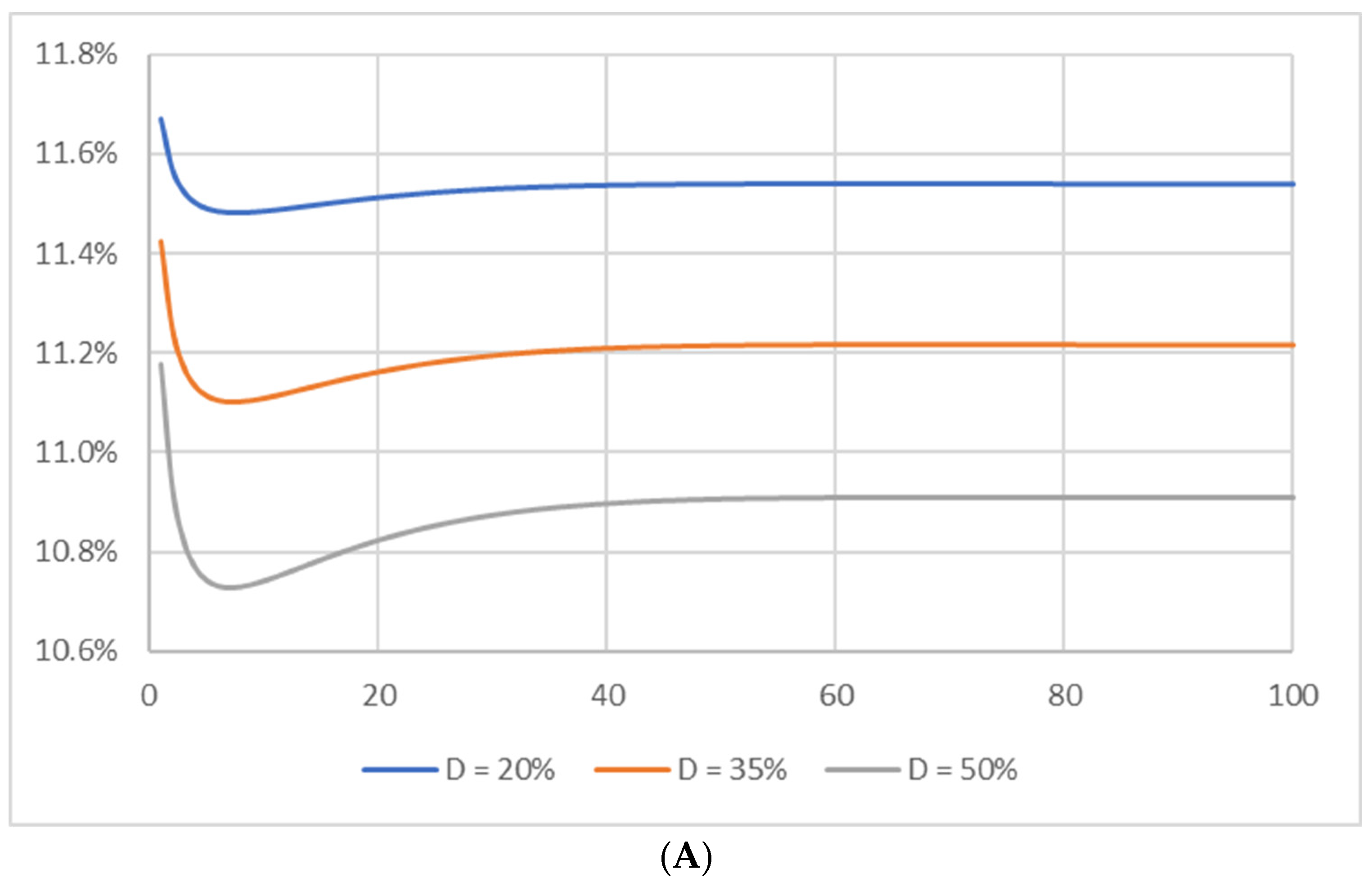
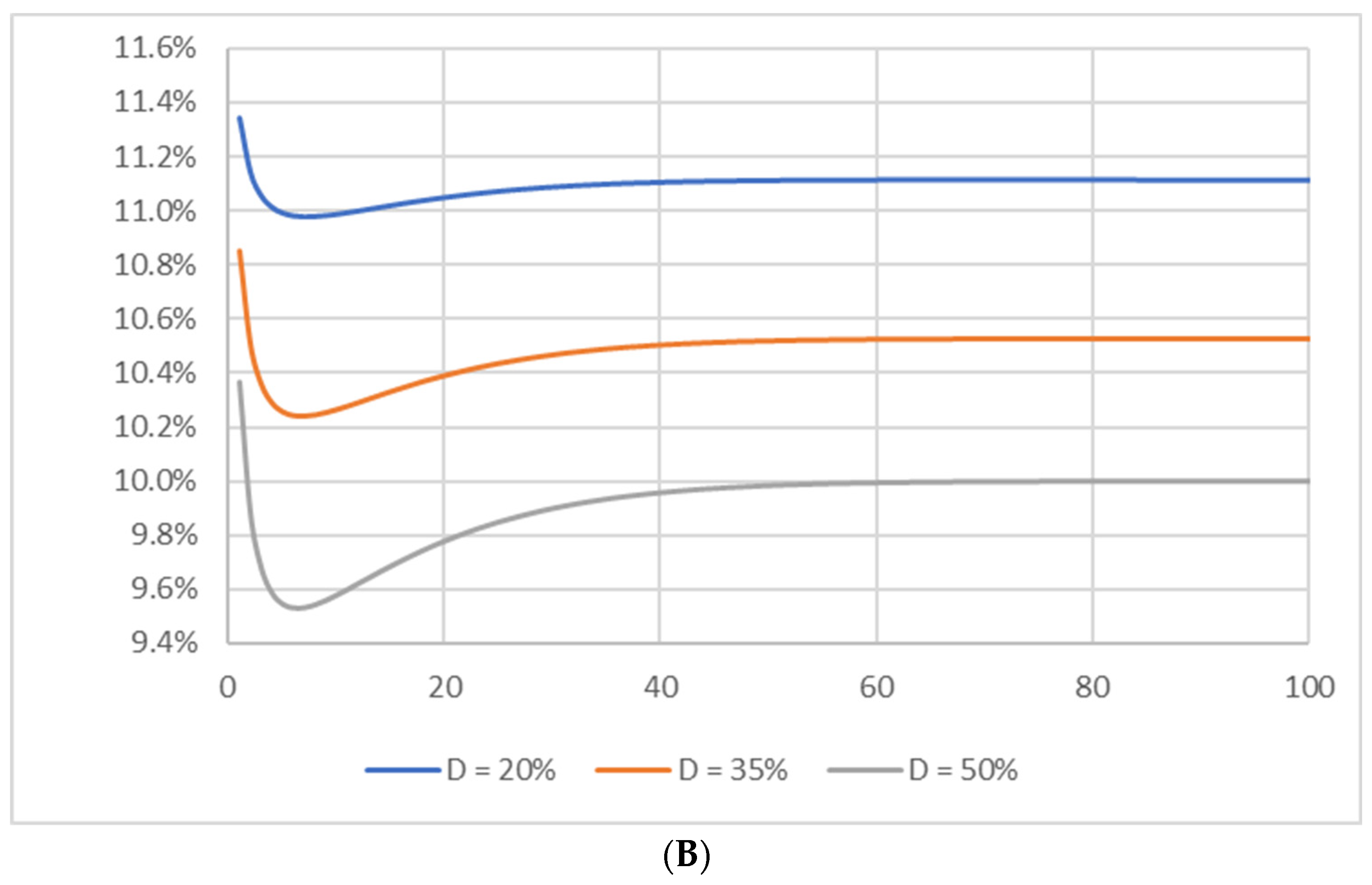
To illustrate this calculation, assume that r_A,U = 10%, r_D = 6%, τ = 20%, V_U = 1000, and D₀ = 200. If N = 10, the unlevered asset will generate a level, free-cash-flow annuity of 162.745 over its useful life. If the debt comprises coupon bonds, the value of the tax shield can be calculated using Equation (6): V_TS = 17.664. The finite-life WACC for this project, WACC₁₀, is the discount rate that sets the present value of the 10-year annuity of 162.745 equal to 1017.664 (=V_L using Equation (1)). This discount rate, 9.594%, also satisfies Equation (8).8 In contrast, WACC_∞ can be calculated using Equation (3) and is 9.615%.9 Clearly, it is possible for the WACC_N to be less than WACC_∞.

As in Brusov et al. (2011), the examples in Section 4.1 illustrate the relations between WACC_N and WACC_∞ when the firm’s debt comprises coupon bonds. The examples in Section 4.2 identify the relations between WACC_N and WACC_∞ when the debt consists of amortizing loans. Within each set of examples, V_U = 1000 and the WACCs are calculated using three levels of debt financing (D₀ = 200, 350, and 500) and two marginal tax rates (τ = 20% and τ = 40%). In each case, it is assumed that the unlevered after-tax cash flow is a level annuity over the assumed useful life.10

Perhaps the most important input, however, is the risk premium—defined herein as the difference between r_A,U and r_D. Unfortunately, there is not a generally accepted answer to the question of how large this risk premium is in practice. Fernandez (2019) finds that 150 textbooks published between 1979 and 2009 recommend equity risk premiums ranging from 3% to 10%. He also reports that the 5-year moving average of these recommendations declined from 8.4% in 1979 to 5.7% in 2009. Fernandez et al. (2021) list the average market risk premium used in 88 countries based upon survey responses. They find that the risk premiums used in the U.S.A. and in the major European countries tend to fall between 5% and 6%. Similarly, Bruner et al. (1998, p. 26) report that most “of our best-practice companies use a risk premium of 6% or lower”. However, the risk premiums referenced in these prior studies are not differences between r_A,U and r_D. Instead, these risk premiums quantify the difference between the levered equity and debt returns.11

Because r_E will typically be greater than r_A,U for a levered firm, the difference between r_A,U and r_D is likely to be smaller than the risk premiums in the Fernandez and Bruner studies. Therefore, the examples herein are calculated using two different risk premium levels: 4% (slightly less than the market risk premium in the U.S.A. and major European countries) and 8% (slightly less than the larger market risk premiums in the Fernandez and Fernandez et al. studies).12

4.1. Coupon Bonds

The examples in this section use the assumption that the debt cash flows mirror those of a coupon bond. The annual interest payment is equal to r_DD₀ with the principal to be repaid at maturity.

Figure 1 graphs estimates of WACC_N assuming that r_A,U = 12% and r_D = 4% (r_A,U − r_D = 8%). In Panel A, τ = 20%. In Panel B, τ = 40%.

Table 3. The Finite-Life WACC with Coupon Bonds (Large Risk Premium). This table provides information about the distribution of WACC_N when r_A,U = 12% and r_D = 4% (r_A,U − r_D = 8%). In particular, the table identifies WACC_N when N = 1, 10, and ∞. In addition, the table lists the implied values of r_E that satisfy Equation (4). Finally, the table identifies the useful life associated with the minimum WACC_N and the range, if any, within which WACC_N is less than WACC_∞. In Panel A, τ = 20%. In Panel B, τ = 40%. Within each panel, this information is presented for three debt levels: D₀ = 200, 350, and 500.

	WACCN (%)				Min. WACC		$\mathit{W}\mathit{A}\mathit{C}{\mathit{C}}_{\mathit{N}} < \mathit{W}\mathit{A}\mathit{C}{\mathit{C}}_{\mathit{\infty }}$
D0	1	10	$\mathit{\infty }$	rE (%)	%	N	Beg N	End N
Panel A: $\tau =20\%$
200	11.83	11.69	11.54	13.52	11.54	$\infty$	NA	NA
350	11.70	11.45	11.21	15.11	11.21	$\infty$	NA	NA
500	11.57	11.23	10.91	17.33	10.91	$\infty$	NA	NA
Panel B: $\tau =40\%$
200	11.66	11.38	11.11	13.09	11.11	$\infty$	NA	NA
350	11.40	10.93	10.53	14.13	10.53	$\infty$	NA	NA
500	11.15	10.49	10.00	15.43	10.00	$\infty$	NA	NA

, Panels A and B, provides additional numerical information about specific data points from the graphs in Figure 1. In particular, Table 3 identifies WACC_N when N = 1, 10, and ∞. In addition, the table lists the implied values of r_E that satisfy Equation (4). Finally, the table identifies the useful life associated with the minimum WACC_N and the range, if any, within which WACC_N is less than WACC_∞.

The implied values of r_E listed in Table 3 range from 13.09% when τ = 40% and D₀ = 200 to 17.33% when τ = 20% and D₀ = 500. Thus, the differences between the implied values of r_E and r_D = 4% range from just less than 10 percentage points to over 13 percentage points and the implied market risk premium falls approximately in, or slightly above, the upper range of potential risk premiums identified in Fernandez (2019) and Fernandez et al. (2021).

In each of the cases illustrated in Figure 1 and Table 3, WACC_N is greater than WACC_∞ for all N < ∞. However, WACC_N decreases rapidly during the years N = 1 to 10—eliminating approximately half of the difference between WACC₁ and WACC_∞—because a disproportionate amount of the perpetual tax shield value, τ D₀, can be attributed to interest payments during those years, as shown in Table 2. The smallest difference between WACC₁₀ and WACC_∞ is when D₀ = 200 and τ = 20% (Panel A): the difference between WACC₁ and WACC_∞ is 0.29 percentage points and the difference between WACC₁₀ and WACC_∞ is 0.15 percentage points. The largest difference between WACC₁₀ and WACC_∞ is when D₀ = 500 and τ = 40% (Panel B): the difference between WACC₁ and WACC_∞ is 1.15 percentage points, and the difference between WACC₁₀ and WACC_∞ is 0.49 percentage points.

Figure 2 graphs finite-life WACC estimates assuming that r_A,U = 12% and r_D = 8% (r_A,U − r_D = 4%). In Panel A, τ = 20%. In Panel B, τ = 40%.

Table 4. The Finite-Life WACC with Coupon Bonds (Small Risk Premium). This table provides information about the distribution of WACC_N when r_A,U = 12%, r_D = 8% (r_A,U − r_D = 4%), and the firm’s debt comprises coupon bonds. In particular, the table identifies WACC_N when N = 1, 10, and ∞. In addition, the table lists the implied values of r_E that satisfy Equation (4). Finally, the table identifies the useful life associated with the minimum WACC_N and the range, if any, within which WACC_N is less than WACC_∞. In Panel A, τ = 20%. In Panel B, τ = 40%. Within each panel, this information is presented for three debt levels: D₀ = 200, 350, and 500.

	WACCN (%)				Min. WACC		$\mathit{W}\mathit{A}\mathit{C}{\mathit{C}}_{\mathit{N}} < \mathit{W}\mathit{A}\mathit{C}{\mathit{C}}_{\mathit{\infty }}$
D0	1	10	$\mathit{\infty }$	rE (%)	%	N	Beg N	End N
Panel A: $\tau =20\%$
200	11.67	11.48	11.54	12.76	11.48	8	3	47
350	11.42	11.11	11.21	13.56	11.10	7	3	53
500	11.18	10.74	10.91	14.67	10.73	7	3	63
Panel B: $\tau =40\%$
200	11.34	10.99	11.11	12.54	10.98	7	3	55
350	10.85	10.27	10.53	13.06	10.24	7	2	68
500	10.36	9.58	10.00	13.71	9.53	6	2	84

, Panels A and B, provides additional numerical information about specific data points from the graphs in Figure 2. The column headings are repeated from Table 3.

The implied values of r_E listed in Table 4 range from 12.54% when τ = 40% and D₀ = 200 to 14.67% when τ = 20% and D₀ = 500. Thus, the differences between the implied values of r_E,∞ and r_D = 8% range from 4.5 percentage points to 6.67 percentage points and the implied market risk premium falls approximately in the lower range of potential risk premiums identified in Fernandez (2019) and Fernandez et al. (2021).

Figure 2 and Table 4 reveal that WACC_N can be less than WACC_∞ over a wide range of N values when the risk premium is 4% and r_D = 8%. In Panel A, WACC_N is less than WACC_∞ for N = 3 through N = 63 when D₀ = 500. However, the maximum difference between the minimum value of WACC_N and WACC_∞ is only 0.18 percentage points. In Panel B, the ranges over which WACC_N is less than WACC_∞ are longer, and the differences between the minimum WACC_N and WACC_∞ are slightly larger. The maximum difference between the minimum value of WACC_N and WACC_∞ is 0.47 percentage points.

As r_D increases and the risk premium r_A,U − r_D decreases, the combination of the following two factors makes it possible for WACC_N to be less than WACC_∞. First, as r_D increases, a greater portion of the perpetual tax shield can be attributed to the earlier interest payments, as shown in Table 2. Second, as the risk premium r_A,U − r_D decreases (holding r_A,U constant), the differences between WACC₁ and WACC_∞ will become smaller at each combination of τ and D₀. For example, the maximum difference between WACC₁ and WACC_∞ in Table 3 (r_D = 4%, τ = 40%, and D₀ = 500) is 1.15 percentage points. In Table 4 (r_D = 8%, τ = 40%, and D₀ = 500), it is just 0.36 percentage points.

As r_D increases and the risk premium r_A,U − r_D decreases, WACC_N will be less than WACC_∞ if V_TS,N exceeds a critical value. To illustrate this, note that when r_A,U = 12%, V_U = 1000, and N = ∞, the perpetual, unlevered, after-tax cash flow is 120. If τ = 40% and D₀ = 500, then V_TS,∞ = 200 and WACC_∞ = 10%. When r_A,U = 12%, V_U = 1000, and N = 10, the perpetual, unlevered, after-tax cash flow is 176.98. For WACC₁₀ to be greater than or equal to 10%, V_L must less than or equal to 1087.49.13 However, when D₀ = 500, τ = 40%, r_D = 8%, and K = 10, V_TS,10 = 107.36, which is calculated using Equation (6). Because V_TS,10 = 107.36 > 87.49, WACC₁₀ is less than 10%.14

The results in Figure 1 and Figure 2 (and Table 3 and Table 4) reveal that when a firm’s debt comprises coupon bonds, the difference between WACC_N and WACC_∞ is likely to be less than one percentage point, especially if N is approximately equal to or greater than 10 years. Nevertheless, the results in Figure 1 and Table 3 suggest that if the market risk premium is large (i.e., 8 percentage points), the use of WACC_∞ when evaluating potential projects can introduce an upward bias into NPV estimates because WACC_∞ is too low. In contrast, if the risk premium is smaller (i.e., 4 percentage points), the results in Figure 2 and Table 4 show that the use of WACC_∞ can introduce either an upward or downward bias into NPV calculations depending on whether WACC_N is higher or lower than WACC_∞. Even though these biases might be small, managers should be aware of their existence before embarking on the sensitivity analysis of a project’s estimated NPV.

4.2. Amortizing Loans

If a firm’s debt comprises amortizing loans rather than coupon bonds, the firm will pay off the debt principal sooner and will pay less interest over time. Thus, the value of a its tax shield will be lower if it issues amortizing loans rather than coupon bonds. The examples in this section compare estimates of WACC_N to WACC_∞ assuming that the firm’s debt comprises amortizing loans.

The examples in

Table 5. The Finite-Life WACC with Amortizing Debt (Large Risk Premium). This table lists values of WACC_N when r_A,U = 12%, r_D = 4% (r_A,U − r_D = 8%), and the firm’s debt comprises amortizing loans. In particular, the table identifies WACC_N when N = 1, 5, 10, 25, 50, 100, and ∞. In Panel A, τ = 20%. In Panel B, τ = 40%. Within each panel, this information is presented for three debt levels: D₀ = 200, 350, and 500.

	WACC Value for Useful Life N (%)
D0	1	5	10	25	50	100	$\mathit{\infty }$
Panel A: $\tau =20\%$
200	11.83	11.82	11.81	11.76	11.67	11.57	11.54
350	11.70	11.68	11.66	11.58	11.44	11.27	11.21
500	11.57	11.55	11.52	11.41	11.21	10.99	10.91
Panel B: $\tau =40\%$
200	11.66	11.64	11.62	11.53	11.36	11.18	11.11
350	11.40	11.37	11.33	11.19	10.93	10.63	10.53
500	11.15	11.11	11.06	10.86	10.52	10.13	10.00

use the assumptions that r_A,U = 12% and r_D = 4%. In Panel A, τ = 20%. In Panel B, τ = 40%. For the debt levels D₀ = 200, 350, and 500, each panel lists WACC_N when N = 1, 5, 10, 25, 50, 100, and ∞.

The results in Table 5 reveal that when a firm’s debt comprises amortizing loans WACC_N will decrease progressively (but not linearly) as N increases from 1 to 100, converging toward WACC_∞. The smallest differences between WACC_N and WACC_∞ in Table 5 are when D₀ = 200 and τ = 20%: the difference between WACC₁ and WACC_∞ is 0.29 percentage points, the difference between WACC₁₀ and WACC_∞ is 0.27 percentage points, the difference between WACC₂₅ and WACC_∞ is 0.22 percentage points, and the difference between WACC₅₀ and WACC_∞ is 0.13 percentage points. The largest differences between WACC_N and WACC_∞ are when D₀ = 500 and τ = 40% (Panel B): the difference between WACC₁ and WACC_∞ is 1.15 percentage points, the difference between WACC₁₀ and WACC_∞ is 1.11 percentage points, the difference between WACC₂₅ and WACC_∞ is 0.86 percentage points, and the difference between WACC₅₀ and WACC_∞ is 0.52 percentage points.

The examples in

Table 6. The Finite-Life WACC with Amortizing Debt (Small Risk Premium). This table lists values of WACC_N when r_A,U = 12%, r_D = 8% (r_A,U − r_D = 4%), and the firm’s debt comprises amortizing loans. In particular, the table identifies WACC_N when N = 1, 5, 10, 25, 50, 100, and ∞. In Panel A, τ = 20%. In Panel B, τ = 40%. Within each panel, this information is presented for three debt levels: D₀ = 200, 350, and 500.

	WACC Value for Useful Life N (%)
D0	1	5	10	25	50	100	$\mathit{\infty }$
Panel A: $\tau =20\%$
200	11.67	11.66	11.65	11.62	11.57	11.54	11.54
350	11.42	11.41	11.40	11.34	11.26	11.22	11.21
500	11.18	11.16	11.14	11.07	10.97	10.91	10.91
Panel B: $\tau =40\%$
200	11.34	11.33	11.31	11.25	11.16	11.11	11.11
350	10.85	10.84	10.81	10.73	10.60	10.53	10.53
500	10.36	10.35	10.33	10.24	10.09	10.01	10.00

use the assumptions that r_A,U = 12% and r_D = 8%. In Panel A, τ = 20%. In Panel B, τ = 40%. For the debt levels D₀ = 200, 350, and 500, each panel lists WACC_N when N = 1, 5, 10, 25, 50, 100, and ∞.

As in Table 5, the results in Table 6 show that when a firm’s debt comprises amortizing loans WACC_N will decrease progressively (but not linearly) as N increases from 1 to 100, converging toward WACC_∞. However, because the differences between WACC₁ and WACC_∞ are smaller in Table 6 than in Table 5, the difference between each WACC_N and WACC_∞ is smaller as well. The smallest differences between WACC_N and WACC_∞ in Table 6 are when D₀ = 200 and τ = 20% (Panel A): the difference between WACC₁ and WACC_∞ is 0.13 percentage points, the difference between WACC₁₀ and WACC_∞ is 0.11 percentage points, the difference between WACC₂₅ and WACC_∞ is 0.08 percentage points, and the difference between WACC₅₀ and WACC_∞ is 0.03 percentage points. The largest differences between WACC_N and WACC_∞ are when D₀ = 500 and τ = 40% (Panel B): the difference between WACC₁ and WACC_∞ is 0.36 percentage points, the difference between WACC₁₀ and WACC_∞ is 0.33 percentage points, the difference between WACC₂₅ and WACC_∞ is 0.24 percentage points, and the difference between WACC₅₀ and WACC_∞ is 0.09 percentage points.

The results in Table 5 and Table 6 reveal that when a firm’s debt comprises amortizing loans, WACC_N is likely to be greater than WACC_∞. Therefore, the use of WACC_∞ can, again, introduce an upward bias into NPV estimates. If the risk premium is large, as in Table 5, the differences between WACC_N and WACC_∞ can approximate or exceed one percentage point, especially when the tax rate is high and the firm uses a substantial amount of debt. If the risk premium is smaller, as in Table 6, the differences between WACC_N and WACC_∞ are likely to be smaller as well. Thus, managers should be aware that the potential magnitude of any distortion to the estimated NPV of a potential project will be related to the size of the risk premium, and guard against overinvestment (e.g., by engaging in additional sensitivity analysis) when the appropriate risk premium is large.

5. What Difference Does the Difference between WACC_N and WACC_∞ Make?

As discussed in Section 2.2, data limitations will make it difficult for managers to estimate a firm’s WACC_∞ with precision. Additional uncertainty is introduced into the capital budgeting process if a project will have a finite useful life, as WACC_∞ (even if accurately measured) can differ from the appropriate discount rate, WACC_N. However, as noted by Miller (2009, p. 137), NPV estimates can also be distorted because a project’s future cash flows cannot be precisely quantified, and these distortions can dwarf those created by the imprecise measurement of the discount rate.

The classic WACC valuation framework requires managers to first estimate the unlevered free cash flows a project will produce over its useful life. Then, the present value of these cash flows must be calculated. The project’s NPV is the difference between this present value and the required initial investment. The following example illustrates the potential distortion to this NPV estimate if WACC_∞, rather than WACC_N, is used as the discount rate.

Assume that a project requires an initial investment in fixed assets of 1000 (assume that the working capital investment is equal to 0), will have a ten-year useful life, and will produce a level amount of earnings before depreciation and taxes in each of the ten years. The investment will be depreciated using the straight-line method over ten years for both book and tax purposes and the tax rate is 40%.

Table 7. The Unlevered Free Cash Flow Calculation. This table shows how to calculate a project’s unlevered free cash flow. Within this example, the pro forma income and cash flow statements are constant across each of the 10 years of the project’s useful life.

Income Statement		Cash Flows
EBTD	220	Net Income	72
Depreciation	−100	+Depr.	100
EBT	120	+/− Δ in WC	0
Taxes (40%)	48	−CapEx	0
Net Income	72	Unlev. FCF	172

shows how to calculate the unlevered free cash flow for this project.

The firm’s (exact) WACC_∞ can be calculated using Equation (3) and the following inputs: r_A,U = 12%, τ = 40%, and D₀ = 500. Thus, WACC_∞ = 10%. For purposes of calculating WACC₁₀, r_D = 8%. If the firm issues coupon bonds, WACC₁₀ = 9.58%. (Table 4, Panel B). If the firm issues amortizing debt, WACC₁₀ = 10.33%. (Table 6, Panel B). Using the assumption that the project produces a ten-year annuity in the amount of 172, the project’s NPV is 56.87 using WACC_∞ = 10%, 76.21 using WACC₁₀ = 9.58%, and 42.05 using WACC₁₀ = 10.33%.

Within this hypothetical example, the NPV is positive using all three discount rates (This of course will not always be the case). However, just because the estimated NPV of a project is positive does not mean that the firm should immediately accept the project. Instead, the decision-maker must recognize that each line item in the pro forma income statement—each year—is an estimate, and one or more of these estimates could prove to be incorrect. Thus, before accepting a project, the manager must evaluate the estimated NPV for reasonableness. What value is created for consumers, allowing the firm to charge premium prices? And if the firm can charge premium prices for the product, rival firms will almost certainly attempt to replicate the product and enter the market. Within this environment, how will the firm construct entry barriers—making it difficult for competitor to enter the market—allowing the project to continue producing positive NPV cash flows into the (distant) future? If the firm cannot identify satisfactory answers to these questions, the firm should not make the investment because future events might reveal that the project’s NPV was not really positive.

6. Conclusions

No project or firm will produce cash flows in perpetuity. As a result, a firm’s perpetuity-formula WACC is unlikely to be the theoretically appropriate discount rate for a project with a finite useful life. However, because the numerical value of the finite-life WACC can be very sensitive to the assumed life of a project, and because it is difficult to estimate the useful life of a project with precision, the finite-life WACC is unlikely to be a viable replacement for the perpetuity-formula WACC within most applications.

The goal of this paper, then, is to help managers better understand the potential biases introduced into the project selection process when the perpetuity-formula WACC is used to evaluate projects with finite useful lives. To do this, the paper compares perpetuity-formula and finite-life WACC estimates across a wide range of input values.

If a firm issues coupon bonds, the finite-life WACC converges quickly toward the perpetuity-formula WACC as the assumed useful life increases from 1 to 5. If the equity risk premium is sizeable (i.e., >8%), the perpetuity-formula WACC is likely to remain lower than (but close to) the finite-life WACC as the useful life extends toward infinity. If the risk premium is smaller (i.e., 4%), the finite-life WACC can be slightly less than the perpetuity-formula WACC across the range of useful lives most likely to be encountered in practice (i.e., between 3 and 50). Thus, if the discount rate in an NPV calculation is viewed as a rough approximation of the true, unobservable discount rate (e.g., + or −1 percentage point from the true rate), the use of the perpetuity-formula WACC is unlikely to materially distort the investment decisions of firms that issue coupon bonds.

If the firm issues amortizing debt, the perpetuity-formula WACC is likely to be less than the finite-life WACC, regardless of whether the risk premium is large or small. These differences are largest when the marginal tax rate is high, when the firm finances a substantial portion of its investments with debt, and when the equity risk premium is large. If any of these conditions are met, managers should be cognizant of the fact that the perpetuity-formula WACC is potentially too low, and guard against overinvestment. In particular, managers should recalculate the project’s estimated NPV after increasing $WAC{C}_{\infty }$ by 1 percentage point or more during the sensitivity analysis phase of the selection process.

The capital budgeting process requires firms to forecast cash flows five, ten, or more years into the future. Because macroeconomic, industry, and firm-specific conditions can change—sometimes dramatically—over these time horizons, cash flow estimates are, at best, approximations of a project’s prospective performance. From this perspective, small differences in the size of the discount rate used to calculate a project’s NPV will simply add to this uncertainty, as long as these differences are randomly distributed around the true, unobservable, discount rate. However, the results herein suggest that this might not always be the case, and that the difference between the finite-life WACC and the perpetuity-formula WACC can be systematically related to factors such as the project’s useful life, the project’s unlevered cost of capital, the firm’s capital structure, the cost of debt, the marginal tax rate, and most important, the debt repayment pattern (e.g., coupon bonds or amortizing loans). By highlighting factors that could pressure the finite-life WACC to be either higher or lower than the perpetuity-formula WACC, the results in this paper can help managers to better understand the potential biases introduced into the capital budgeting process when using the perpetuity-formula WACC to evaluate projects with finite useful lives.

References

1. Arditti, Fred D. 1973. The Weighted Average Cost of Capital: Some Questions on Its Definition, Interpretation and Use. Journal of Finance 28: 1001–8. [Google Scholar] [CrossRef]
2. Barbi, Massimiliano. 2012. On the Risk-Neutral Value of Debt Tax Shields. Applied Financial Economics 22: 251–58. [Google Scholar] [CrossRef]
3. Booth, Laurence. 2002. Finding Value Where None Exists: Pitfalls in Using Adjusted Present Value. Journal of Applied Corporate Finance 15: 95–104. [Google Scholar] [CrossRef]
4. Brick, John R., and Howard E. Thompson. 1978. The Economic Life of an Investment and the Appropriate Discount Rate. Journal of Financial and Quantitative Analysis 13: 831–46. [Google Scholar] [CrossRef]
5. Bruner, Robert F., Kenneth M. Eades, Robert S. Harris, and Robert C. Higgins. 1998. Best Practices in Estimating the Cost of Capital: Survey and Synthesis. Financial Practice and Education 8: 13–28. [Google Scholar]
6. Brusov, Peter, Tatiana Filatova, Natali Orehova, and Nastia Brusova. 2011. Weighted Average Cost of Capital in the Theory of Modigliani-Miller, Modified for a Finite Lifetime Company. Applied Financial Economics 21: 815–24. [Google Scholar] [CrossRef]
7. Campani, Carlos Heitor. 2015. On the Correct Evaluation of Cost of Capital for Project Valuation. Applied Mathematical Statistics 9: 6583–6604. [Google Scholar] [CrossRef]
8. Cooper, Ian A., and Kjell G. Nyborg. 2006. The Value of Tax Shields IS Equal to the Present Value of Tax Shields. Journal of Financial Economics 81: 215–25. [Google Scholar] [CrossRef]
9. Farber, André, Roland L. Gillet, and Ariane Szafarz. 2006. A General Formula for the WACC. International Journal of Business 11: 211–18. [Google Scholar]
10. Fernandez, Pablo. 2004. The Value of Tax Shields is NOT Equal to the Present Value of Tax Shields. Journal of Financial Economics 73: 145–65. [Google Scholar] [CrossRef]
11. Fernandez, Pablo. 2007. A General Formula for the WACC: A Comment. International Journal of Business 12: 399–403. [Google Scholar]
12. Fernandez, Pablo. 2019. The Equity Premium in 150 Textbooks. Available online: https://ssrn.com/abstract=1473225 (accessed on 15 March 2023).
13. Fernandez, Pablo, Sofía Bañuls, and Pablo F. Acín. 2021. Survey: Market Risk Premium and Risk-Free Rate Used for 88 Countries in 2021. IESE Business School Working Paper. Available online: https://ssrn.com/abstract=3861152 (accessed on 15 March 2023).
14. Filatova, Tatiana, Brusov Peter, and Natali Orekhova. 2022. Impact of Advance Payments of Tax on Profit on Effectiveness of Investments. Mathematics 10: 666. [Google Scholar] [CrossRef]
15. Haley, Charles W., and Lawrence. D. Schall. 1973. The Theory of Financial Decisions. New York: McGraw-Hill. [Google Scholar]
16. Magni, Carlo Alberto. 2010. Average Internal Rate of Return and Investment Decisions: A New Perspective. The Engineering Economist 55: 150–80. [Google Scholar] [CrossRef]
17. Magni, Carlo Alberto. 2013. The internal-rate-of-return approach and the AIRR paradigm: A refutation and a corroboration. The Engineering Economist 58: 73–111. [Google Scholar] [CrossRef]
18. Magni, Carlo Alberto. 2016. Capital Depreciation and the Underdetermination of Rate of Return: A Unifying Perspective. Journal of Mathematical Economics 67: 54–79. [Google Scholar] [CrossRef]
19. Magni, Carlo Alberto. 2020. Investment Decisions and the Logic of Valuation. Linking Finance, Accounting, and Engineering. Cham: Springer Nature Switzerland AG. [Google Scholar]
20. Miles, James A., and John R. Ezzell. 1980. The Weighted Average Cost of Capital, Perfect Capital Markets, and Project Life: A Clarification. Journal of Financial and Quantitative Analysis 15: 719–30. [Google Scholar] [CrossRef]
21. Miller, Richard A. 2009. The Weighted Average Cost of Capital is Not Quite Right. The Quarterly Review of Economics and Finance 49: 128–38. [Google Scholar] [CrossRef]
22. Modigliani, Franco, and Merton H. Miller. 1958. The Cost of Capital, Corporation Finance and the Theory of Investment. American Economic Review 48: 261–97. [Google Scholar]
23. Modigliani, Franco, and Merton H. Miller. 1963. Corporate Income Taxes and the Cost of Capital: A Correction. American Economic Review 53: 433–43. [Google Scholar]
24. Myers, Stewart C. 1974. Interactions of Corporate Financing and Investment Decisions—Implications for Capital Budgeting. Journal of Finance 29: 1–25. [Google Scholar] [CrossRef]
25. Pierru, Axel. 2009. The Weighted Average Cost of Capital is Not Quite Right: A Comment. The Quarterly Review of Economics and Finance 49: 1219–23. [Google Scholar] [CrossRef]
26. Reilly, Raymond R., and William E. Wecker. 1973. On the Weighted Average Cost of Capital. Journal of Financial and Quantitative Analysis 8: 123–26. [Google Scholar] [CrossRef]
27. Welch, Ivo. 2021. The Cost of Capital: If Not the CAPM, then What? Management and Business Review 1: 187–94. [Google Scholar]
Figure 1. Coupon Bonds and the Finite-Life WACC when the Risk Premium is Large. This figure graphs values of WACCN, for N = 1 to 100, when rA,U = 12%, rD = 4% (rA,UrD = 8%), and the firm’s debt comprises coupon bonds. In (A) τ = 20%. In (B) τ = 40%. Within each panel, this information is graphed for three debt levels: D0 = 200, 350, and 500.
Jrfm 16 00398 g001
Figure 2. Coupon Bonds and the Finite-Life WACC when the Risk Premium is Small. This figure graphs values of WACCN, for N = 1 to 100, when rA,U = 12%, rD = 8% (rA,UrD = 4%), and the firm’s debt comprises coupon bonds. In (A) τ = 20%. In (B) τ = 40%. Within each panel, this information is graphed for three debt levels: D0 = 200, 350, and 500.
Jrfm 16 00398 g002aJrfm 16 00398 g002b