Abstract
Storage profit maximization is based on buying energy at the lowest prices and selling it at the highest prices. The best strategy must thus be based on both accurately predicting the price peak hours and on rightly choosing when to buy and when to sell the stored energy. In this aim, price prediction is crucial, but choosing the prediction model by means of the usual metrics, as the lowest mean squared error, is not an effective solution as the mean squared error computation equally weights the prediction error of all prices, while the focus must be on the higher and lower prices. In this paper, we propose a new metric focused on the correct forecasting of high and low prices so as to allow for a more effective choice among price forecasting models. Results show that the new metric outperforms the standard metrics, allowing for a more accurate estimation of the possible profit for storage (or other trading) activities.
1. Introduction
The introduction of higher shares of renewable energy source (RES)-based electricity production is the main target of the energy transition process. Currently, the main share of RESs is not programmable and therefore not adaptable to consumption needs. Storage technologies are one of the key points for narrowing the mismatch between RES production and consumption curves, transferring part of the energy from the production peak hours to the consumption peak hours.
The technical need described above is rightly coupled, in economic terms, with storage operator profit maximization, as it can be reached by buying energy at the lowest prices (correspondent to production peaks) and selling it at the highest prices (consumption peaks). In this way, the storage activity can reduce the mismatch between production and consumption timing so as to allow for a higher share of RES production.
A specific characteristic of electricity markets is that electricity consumption and production must always be in equilibrium. Thus, the markets must fix the actual production and consumption quantities and prices at any moment. Two basic models for power markets were developed, one based on a day-ahead auction, where prices and generation amounts for the 24 h of the following day are determined by an auctioning process, and real-time markets, where continuous trading is allowed until shortly before delivery. Markets in Australia, Canada, and Singapore are based on real-time trading, while those in the US, Korea, India, and Russia are mainly based on day-ahead auctions Mayer and Trück (2018). Since the years around 2000, after a comprehensive energy market deregulation, the European Union markets have been based on day-ahead auctions, with intraday real-time markets as a secondary trading platform. In Italy, due to the power grid structure, the day-ahead auction market is organized by regional zones and is managed by “Gestore Mercati Energetici” (GME), a state-managed company.
In the Italian day-ahead auction, for each hour of the next day, each producer proposes its offer, specifying the requested minimum price and the power quantity for the supply, and each distributor proposes its offer specifying the maximum acceptable price and the demanded quantity. The auction mechanism then identifies the clearing price, which equilibrates demand and supply and will be paid to all accepted producers by all accepted distributors.
Storage profit maximization is based on buying energy at the lowest prices and selling it at the highest prices. This means that the best strategy must be based on both accurately predicting the price peak hours and on rightly choosing when to buy and when to sell stored energy. In a previous work Sbaraglia et al. (2024), we developed a model and software infrastructure for simulating a storage business operator in the Italian energy market.
The optimal buy/sell strategy for the storage operator is a highly nonlinear process, whose maximum profit can just be computed a posteriori at known prices, while the actual best strategy must be chosen among some realistic strategies that can be implemented in practice.
Even when assuming, in a first approximation, that the storage operator is a price taker in that its buy/sell activity does not influence the prices, determining the best operator strategy is not straightforward.
In this aim, price prediction is crucial, so the key point is in selecting the best price forecasting method. If this selection is based on the usual statistical metrics, such as the mean squared error (MSE), the outcome may not be the best solution. In fact, the profit maximization must be based on accurately forecasting the higher and lower prices, which is not in line with the mean squared error metric, whose aim is on equally considering prediction errors in all prices. Thus, some other metric must be considered, and profit maximization should be the target of the price forecasting evaluation metric.
In this paper, we introduce a new metric designed to improve the accurate forecasting of high and low prices, enabling a more effective selection of price forecasting models. The results demonstrate that the proposed metric outperforms standard metrics, providing a more precise estimation of potential profits for storage or other trading activities.
The reminder of this paper is structured as follows. Section 2 presents the literature review, Section 3 describes the optimization model, Section 4 describes the standard accuracy metrics and introduces our proposed new alternatives, Section 5 presents the price forecasting methods used in the simulation, Section 6 reports the simulation results, and Section 7 draws the conclusions.
2. Literature Review
Accurate price forecasting plays a critical role in the profitability of storage operators, who rely on this information to make optimal trading decisions. Price forecasts directly impact their ability to generate profits through arbitrage trading, that is, by buying/storing during low-price periods and selling during high-price periods. This is even more true in day-ahead electricity markets, where all participants submit their trading orders before electricity is generated and consumed on the next day. Because of this importance, the corresponding literature on price forecasting models is vast and constantly evolving. A comprehensive review of these works is beyond the scope of this paper, but valuable insights are provided by Cerjan et al. (2013), Weron (2014), Nowotarski and Weron (2018), Acaroğlu et al. (2021), Lago (2021), Lu et al. (2021), and Zema and Sulich (2022).
In the following, we explore evolving trends in price forecasting methods, emphasizing recent contributions relevant to the scope of this paper, particularly those tailored to day-ahead electricity markets.
Price forecasting models can be broadly categorized into two main groups: conventional models and AI-based models. The first group includes time-series statistical models such as ARIMA and GARCH, which are extensively utilized for their ability to capture linear patterns and rely on historical price data. In extensive evaluations of price forecasting methods, Makridaki et al. (2018) and Parmezan et al. (2019) find that ARIMA is more computationally efficient than machine learning algorithms and can outperform them in specific scenarios despite requiring more extensive parameterization. Zou and Yang (2004) combine multiple econometric models to improve forecasting accuracy, updating their weights after each observation and demonstrating better performance compared to using a single model. Focusing on electricity price forecasting, Ghasemi et al. (2021) highlight the effectiveness of ARIMA in short-term electricity price forecasting, while Ziel and Steinert (2018) discuss the applicability of GARCH models for managing price volatility. Recent contributions to intraday electricity markets include the econometric model proposed by Kiesel and Paraschiv (2017), while Uniejewski et al. (2019) address this using the least absolute shrinkage and selection operator (LASSO), a method for estimation in linear models originally proposed by Tibshirani (1996).
Although statistical models have been widely and successfully applied to electricity price modeling, they can struggle to capture complex and nonlinear patterns. To address this limitation, AI-based models have increasingly gained prominence over the past few decades, thanks to their ability to model complex and nonlinear relationships, especially under volatile conditions. AI-based models can be effectively integrated with conventional statistical models, creating hybrid approaches that leverage the strengths of both methodologies. By addressing the limitations of individual models, these hybrid approaches excel in capturing both linear and nonlinear patterns, often resulting in enhanced predictive performance. Hybrid models can also be constructed by combining different AI-based techniques: for example, Rafiei et al. (2016) employ clonal selection, wavelet transform, and extreme learning machines for probabilistic electricity price forecasting. Nowotarski and Weron (2018) provide a comprehensive review on AI-based methods and their hybrid variants. Early models integrating ARIMA and artificial neural networks (ANNs) are proposed by Zhang (2003) and Babu and Reddy (2014), while Panigrahi and Behera (2017) develop a model that combines exponential smoothing with ANN for enhanced time series forecasting. Chaâbane (2014) jointly uses ARFIMA and neural network models for electricity price prediction. Bissing et al. (2019) and Alkawaz et al. (2022) explore hybrid approaches for forecasting hourly day-ahead electricity prices by integrating multiple linear regression and machine learning techniques. Kapoor and Wichitaksorn (2023) compare statistical methods with machine learning approaches for price forecasting in the intraday New Zealand market, concluding that statistical methods, when coupled with LASSO, can outperform machine learning models. Jiang et al. (2025) integrate the LASSO statistical method with neural networks and decision tree-based models for electricity price forecasting; see also Shen et al. (2019). Hybrid models for electricity price forecasting, which adopt a rolling window approach to ensure that the model is trained on the most recent data, are proposed by Papaioannou et al. (2016), Ugurlu et al. (2018), and De Marcos et al. (2019), while Gunduz et al. (2023) further enhance this approach by integrating neural networks with a transfer learning framework. Fezzi and Mosetti (2020) examine the optimal length of the rolling window, highlighting its impact on prediction accuracy.
A parallel area of research to price forecasting methods focuses on evaluating their effectiveness in generating profits, particularly in the context of arbitrage trading strategies. This involves not only predicting price movements accurately but also ensuring that these predictions translate into profitable trading opportunities. This issue has been widely discussed in the financial market literature, as described by Li and Bastos (2020). However, it has received comparatively little attention in the electricity market literature, where performance evaluation typically centers on minimizing forecast errors against historical price data, relying on standard statistical accuracy metrics, as noted by Ziel and Steinert (2018), Beigaite et al. (2018), and Belenguer et al. (2025). The common assumption is that improving forecast accuracy will lead to better arbitrage opportunities and, consequently, higher profits; see, for example, Yu and Foggo (2017) and Mercier et al. (2023). However, recent research suggests that this relationship may not be straightforward, as pointed out by Antweiler (2021), while Jędrzejewski et al. (2022) advocate for further research on improving metrics in the electricity price forecasting literature.
Our work contributes to this emerging area by specifically addressing this gap. Building on existing research, we go beyond evaluating forecasting models solely based on their ability to fit historical prices. Hence, we propose a new metric that simultaneously evaluates the statistical accuracy and economic utility of forecasting methods, particularly for storage operators seeking to maximize arbitrage profits. This dual focus—on both predictive accuracy and economic utility—offers a more comprehensive way of assessing forecasting methods, particularly for participants in electricity markets who rely on forecasts to guide arbitrage decisions.
3. Optimization for the Storage Operator
In Sbaraglia et al. (2024), we proposed an optimization model designed for obtaining the maximum profit from the energy storage business, that is, buying and selling energy at the best market conditions.
The model assumes that the energy market is perfectly liquid, meaning it is always possible to buy and sell the desired quantity of energy at any hour, up to a maximum limit. Furthermore, the storage operator is a price taker; that is, its actions do not influence the market price.
The model, based on the market price of energy at each hour, the maximum storage capacity, and the maximum amount of energy that can be transferred (purchased or sold) in a single hour and some other technical parameters, allows choosing the amount of energy to be purchased or sold at each hour.
The resulting optimization problem consists of maximizing the sum of total revenues from the trading activity. Solving this optimization problem consists of finding the best decision strategy over the set of all admissible strategies, that is, all the allocation strategies that satisfy the above constraints.
The problem is stochastic in nature, since the future evolution of the energy prices, upon which the allocation strategy depends, is unknown. In practice, it is often appropriate to reduce this stochastic optimization problem to a deterministic one by assuming a specific scenario of evolution of the energy prices. In fact, the operator or practitioner can often provide a specific prediction of how the prices will evolve, at least in the short term, and is interested in determining the optimal strategy according to such prediction. The deterministic optimization problem thus obtained, due to its linearity, can be efficiently solved through well-known mixed-integer linear programming algorithms.
Since the energy market requires each operator to participate daily in auctions for every hour of the following day, it is natural for operators to optimize their decisions across the next 24-h period. While a day-by-day optimization approach might yield inferior results compared to a global optimization over the entire simulation period, extensive tests conducted by Sbaraglia et al. (2024) for the Sardinian electricity market during 2019–2023 show that the difference in profits is negligible, and this finding aligns closely with the results of Connolly et al. (2011).
What actually makes a difference is instead price forecasting, with prediction errors that can induce a loss of no less than 15% from the maximum theoretical income at given prices. Thus, the selection of the best price forecasting model is a key point.
4. Price Forecasting Metrics
We intend to evaluate the accuracy of price prediction using as our ultimate benchmark the difference between the theoretical maximum revenue (i.e., the revenue that can be obtained if we assume perfect knowledge of the future prices) and the actual revenue obtained by applying the optimal strategy to the forecasted energy prices.
Let be the actual price function and be the price function as predicted by a given price forecasting method. Furthermore, given the simulation time steps , let be the actual prices, which we shall shortly denote and let be the predicted price curve.
Let be the final revenue obtained by applying the optimal allocation strategy to the actual price curve, thus assuming perfect knowledge of the future. Furthermore, let be the final revenue obtained by applying the optimal strategy to the forecasted energy prices . Clearly, as is the theoretical maximum revenue, we always have . We shall assume as the benchmark to evaluate the accuracy of the price prediction the quantity
Clearly, , and the closer to 0, the better the price forecasting method. We regard as the percentage loss of profit due to imperfect knowledge of the evolution of the energy prices.
While represents the ultimate benchmark in evaluating the accuracy of a price prediction, computing such a metric involves a computationally intensive optimization to determine the final revenue for both the actual and forecasted prices. Furthermore, following this approach does not necessarily shed more light on the characteristics of a given forecasting method that make it more efficient than others. Thus, in this section, we aim to develop simpler price forecasting metrics tailored to the storage optimization model. Such tailored metrics would allow us to measure the forecasting accuracy of each forecast when coupled with the optimal storage allocation strategy, without requiring the computation of the final revenues. Furthermore, since the architecture of our simulation software allows for these metrics to be fed as feedback to the price forecasting module, the latter could use them to refine the forecast for a better fit. Finally, determining accurate price forecasting metrics will provide a better insight in the internals of the optimal storage allocation strategy and how this is impacted by the different characteristics of the price curve.
We shall also compare these tailored custom indicators to some well known statistical loss functions used in the analysis of regression models. Loss functions compare the model’s predicted values with actual values, gauging its efficacy in mapping the relationship between (prediction) and P (target). Loss functions are then functions of the type
such that represents a measure of the accuracy of the prediction, indicating the disparity between predicted and actual values.
The standard loss functions used to evaluate each forecasted time series are described in Appendix A, while the innovative functions we propose and test in comparison to these standard techniques are detailed below.
MaxMin Loss Function
Since the storage operator profits on the price differences, buying when the price is lower and selling when the price is higher, the first simple idea is to approximate such revenue with the price difference between local extrema. Thus, we compare in this metric the approximated revenue when the extrema are identified on the actual price curve vs. the approximated revenue when the extrema are identified on the forecasted price curve. While we do not expect this simplistic model to accurately represent profit, it is still interesting to understand how far such a basic strategy is from optimal before we launch into more sophisticated loss functions.
Let such that and are points of local maximum and minimum, respectively, for the price curve , with . We further assume , shifting the local maxima as necessary and possibly skipping some of them if this is not the case.
In much a similar way we define the local maxima and minima for the estimated price curve so that such that are points of local maximum and minimum, respectively, for the price curve , with and . We define the MaxMin loss function as
Clearly, the closer to zero the metric, the better the forecasted price curve.
Sort Loss Function
While the MaxMin Loss Function could provide some insight towards assessing the accuracy of a price curve prediction, if we look more closely at the optimal allocation strategy for a given price sequence, it is clear that the storage operator does not profit purely on local extrema. In fact, the operator could buy energy at the beginning of the increasing cycle and sell at the end of it, thus realizing a net income, even in absence of local extrema. We, therefore, wish to further refine the MaxMin metric by trying to assess how well the prediction identifies the intraday sorting of the price curve. It is worth reminding that the operator strategy proceeds 24 h at a time, since at any given day the strategy must be defined for the following day. We should therefore split the price curve in chunks of 24 h and compare the intraday sorting of the actual prices vs. the sorting of the predicted prices. The closer the two, the better the forecasted curve should be. If the predicted price curve had an identical sorting of the intraday prices, we should expect an identical optimal strategy, irrespective of the values of the prices themselves.
Let be the simulation days and the daily hours. Let us also recall that all days have been standardized to a uniform 24-h format to neutralize the impact of Daylight Saving Time adjustments. Let be the total number of time steps. For any , let be a sorting of the time hours of day i such that . Now, let be the corresponding sorting of the time hours of day i, determined based on the estimated price curve: .
Now, let , if and if and
Clearly, represents the number of times, in day i, that the sorting of the forecasted price curve is in accordance with the sorting of the actual price curve. We shall then pose
as the percentage of incorrectly identified sorted times. The closer to 0 such a loss function is, the better the forecasted price curve is at predicting the intraday sorting of the prices.
Multistep Loss Function
The sort metric described above measures the sorting of the price curve, day by day, with the assumption that if two price curves are sorted identically the optimal strategy will be the same whatever the values of the prices. However, if the sorting is not completely accurate, the difference in revenue could still be low: since the optimal strategy will basically use the sorting to decide when to buy/sell energy, if the sorting is slightly off but the price difference is small, the difference in profit might be negligible. This is the case, for example, if the forecasted price curve is slightly shifted with respect to the actual prices. In such situations, the sort metric will yield a very high value which does not fully reflect the actual difference in profit. In order to further improve upon the sort metric for a more accurate evaluation of the price curve prediction, we have developed the multistep loss function, which takes into account the value differences in addition to the ordering of the prices.
Let be the simulation days and the time steps within day i. The optimal storage allocation strategy should maximize the intraday price differences; thus, let us consider a disposition without repetition of an even number of time steps and let us call this disposition , . Let us further assume for . The assumption here is that we shall buy at each time and sell at each time , and thus the estimated day i profit resulting from the disposition shall be
The optimal strategy must attain at least the maximum estimated revenue:
where is the set of all dispositions of elements out of the time steps of each day i, , such that for . The total estimated profit over is then
Now, if is a forecasted price curve, we can similarly define, for any disposition as described
and then determine the disposition that achieves the maximum over all dispositions in :
Then, we can compute the estimated profit if such disposition , optimal on the estimated curve, were to be used on the real price curve:
and the resulting total estimated profit over all time steps
The multistep loss function is then simply
Algorithmically, the multistep loss function can be computed by sorting the price curve within each day. Then, iteratively, the maximum sorted time step (highest price) is labeled as “sale time” provided that there is a preceding time step with a lower price. If so, we shall pick as “buying time” the time step preceding the “sale time” which has the lowest price. Thus, the multistep loss function is effectively an evolution of the sort function: where the sort function simply aims at identifying the intraday sorting of the price curve, upon which the profit depends, without any attempt to estimate the corresponding profit, the multistep metric similarly depends on the sorted price curve to establish a profit by exploiting the intraday price differences but aims at estimating the resulting profit. It is intuitive that the multistep estimate of profit is not the actual profit, since the optimal operator strategy might exploit the maximum energy that can be stored, which is usually higher than the maximum that can be transferred within one hour, to implement more efficient sequences of the type “buy–buy–sell”. We shall investigate in Section 6.2 how effective the multistep metric is at predicting profit.
5. Price Forecasting Methods
Several models have been explored for electricity price forecasting, with comprehensive summaries provided in Weron (2014) and Lu et al. (2021). In this work, our focus is to evaluate the effectiveness and reliability of forecasting quality metrics within the context of a storage business. To this end, we selected some of the most commonly used time series-based methods. It is important to note that for each forecasting model, the corresponding daily income must be calculated, making the process computationally intensive. Incorporating more complex models, such as neural networks, would significantly extend the computation time. Additional details on the price forecasting methods can be found in Appendix B. In a previous study Sbaraglia et al. (2024), we delved deeper into these methods and their interaction with both optimal and suboptimal operator strategies. Exploring more advanced forecasting models, including machine learning and RNNs, is a key focus of our ongoing research.
In our testing, we consider both heuristic methods based on intuitive guidelines to predict future prices and econometric methods based on statistical and mathematical models to analyze historical data, offering a more complex, data-driven approach to price forecasting.
The heuristic price forecasting methods that we considered are described as follows.
Today model: this simple approach is straightforward and assumes day-to-day price stability, predicting that the electricity price at any given hour will be the same as it was at the same hour the previous day.
Todaymod model: this model is a variation of the Today method: for Saturdays, Sundays, and Mondays, the Todaymod model predicts that electricity prices at each specific hour will match those from the corresponding day and hour of the previous week. For Tuesdays through Fridays, the model predicts that prices at each specific hour will be the same as those observed at the same hour on the immediately preceding day.
Avg model: for each hour of the day over a defined market period, the forecasted energy price at hour i is calculated by averaging the electricity prices for that same hour across the past K days (with K assumed equal to 30 days).
Avg sameday model: similar to the Avg model, this approach averages the prices for the same hour on the same weekday over the past K weeks (with K assumed equal to 4 weeks).
On the other hand, the econometric methods that we use for forecasting hourly electricity prices are based on the appropriate ARIMA and SARIMA models, selected using the Akaike Information Criterion (AIC). Specifically, we evaluate the time series data for each hour independently, identifying the optimal model parameters for ARIMA and for SARIMA by minimizing the AIC score. This process involves testing all parameter combinations, with values ranging from zero to seven. The hourly price data from 2018 to 2023 have been segmented into 24 distinct time series, one for each hour of the day. For each time series, the best-fitting ARIMA/SARIMA models have been identified for each year. Given the presence of a weekly price cycle, the seasonal period for SARIMA is set to 7 for each hourly time series. Based on this selection process, we predict the hourly electricity price using the following econometric methods.
ARIMA Hourly/SARIMA Hourly: Using a ‘multi-set’ strategy, we forecast hourly prices for each year based on the best model parameters identified for each specific hour in the preceding year. This method captures the unique price fluctuations for each hour by using a distinct model for each one.
ARIMA Modal/SARIMA Modal: This ‘one-set’ approach uses a single set of model parameters, consisting of the modal (most frequently optimal) parameters among the 24 hourly models from the previous year. This approach aims for a more generalized forecast across all hours, relying on the most common optimal parameters. In other words, the method “modal” selects the value that appears most frequently as optimal in the dataset consisting of the set of hours, in contrast to the hourly method, which instead favors the specific optimal value for each individual hour.
We generate all econometric forecasts using the aforementioned methods under a rolling-window approach, which involves retraining the model on a shifting 365-day window of the most recent data. For example, to predict the price for a specific hour on 2 January 2019, the model utilizes data from that same hour spanning from 2 January 2018, to 1 January 2019, with the window advancing accordingly.
Rolling window methods are commonly employed in time series forecasting due to their adaptability and ability to incorporate recent data while discarding older information. This makes them particularly useful in volatile environments where trends can shift quickly. For instance, in the context of energy price forecasting, rolling windows allow for continuous model updates, enhancing accuracy as they respond to real-time data changes. These methods are particularly beneficial in cases where seasonality or cyclical trends are present, as they allow the model to adapt to the most recent trends rather than relying on long-term averages. See also Papaioannou et al. (2016), Ugurlu et al. (2018), De Marcos et al. (2019), Gunduz et al. (2023), and Fezzi and Mosetti (2020). We have observed that a training set of a rolling window of 1 year (365 observations) is enough to produce satisfactory results, as also pointed out by Papaioannou et al. (2016) in the context of energy price forecasting.
6. Results
6.1. Profitability of Standard Price Forecasting Methods
For each price forecasting method outlined in Section 5, we computed the hourly electricity prices from 2019 to 2023 in the Sardinian day-ahead electricity market. Utilizing the profit optimization model detailed in Section 3, we calculated the optimal daily profits achievable by applying each forecasting method.
The simulation setup that we adopted refers to a battery energy storage system (BESS) consisting of a small Lithium-Ion battery plant with a total capacity of 4 MWh, capable of charging or discharging 1 MWh per hour. The hourly maintenance costs of the BESS have been set to EUR /MWh, with no storage losses, transaction costs, or cost of storage. These assumptions are consistent with those adopted by Sbaraglia et al. (2024) and Agathokleous et al. (2019), as well as with the findings of Münderlein et al. (2019) regarding the minimum capacity required for a BESS to cover its operating costs.
The total annual profits attributable to each price forecasting method are presented in Table 1.

Table 1.
Revenue for each forecasting method (nominal values in euro).
Table 2 reports the percentage with respect to the maximum theoretical performance attainable if perfect knowledge of the future prices were available. To ease the comparison, we have colored in red performance below , in orange performance between and , in yellow between and , and in green a percentage higher than . Figure 1 provides the same information in a more immediate, graphical form.
Table 2.
Revenue percentage of theoretical maximum for each forecasting method.
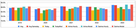
Figure 1.
Revenue percentage of theoretical maximum for each forecasting method.
We can observe how most methods yield within of maximum profit, with some methods achieving as high as in some years.
Our tests reveal clear profit performance patterns across the forecasting methods examined. Within the heuristic category, the Avg and Avg Sameday models, which derive forecasts from average prices, mostly outperform models like Today and Todaymod, which depend on the most recent corresponding price data. This indicates that models based on averages are more effective at capturing and utilizing historical price trends to secure more profitable outcomes.
A parallel trend is observed among the econometric forecasting methods, where a preference for simplicity and a general approach is evident. The “one-set” approach, as implemented by the ARIMA Modal and SARIMA Modal models, involves applying a consistent set of optimal parameters across all hourly forecasts. This method consistently yields higher profits compared to the ’multi-set’ approach of the ARIMA Hourly and SARIMA Hourly models, which customize optimal parameters for each specific hour. The success of the “one-set” approach in generating profits highlights the strength of a broad, generalized modeling framework. Far from diminishing profitability, the simplicity of this approach seems to enhance it, likely due to its robustness and wide applicability across various times. These findings challenge the assumption that more complex, hour-specific customization leads to better performance, suggesting instead that a streamlined, uniform approach to parameter selection in econometric forecasting can be more effective in maximizing profits.
When comparing the top-performing models within each category (namely, the Avg and Avg Sameday for heuristic approaches, and the ARIMA Modal and SARIMA Modal for econometric strategies), no single method consistently dominates in terms of profitability. This variation suggests that the most effective model depends on the specific market conditions at play.
Specifically, the heuristic methods of Avg and Avg Sameday show superior profitability during years marked by significant exogenous shocks, such as the widespread effects of the COVID-19 pandemic in 2020 and the gas price crisis triggered by the Russia–Ukraine war in 2022. These models excel in rapidly adjusting to and capitalizing on abrupt market changes for short-term gain.
In contrast, the econometric models (ARIMA Modal and SARIMA Modal) demonstrate their strength in more stable or predictable market environments, as seen in the years 2019, 2021, and 2023. Their advantage lies in incorporating long-term historical price data, which allows them to regain and even enhance profitability once the immediate impacts of exogenous events have been assimilated into the broader price trends. This distinction suggests that while heuristic methods may offer immediate advantages by quickly responding to sudden market shifts, econometric approaches provide consistent guidance, gradually adjusting to include new data trends and thus, over time, recapturing profitability in the aftermath of such events.
Given that no forecasting method emerges as more accurate over all years and conditions, it is clearly not possible to determine in advance which will yield higher accuracy. Thus, adaptive methods able to dynamically switch from one forecast to the other based on the evaluation of past performance could be appealing. However, the actual implementation of such methods would require an iterative evaluation of each of many forecasting methods over the past K days in order to determine which strategy to use for the following K days. Such an algorithm would easily be computationally demanding since it requires running multiple global optimization for each method and for each K step interval. Hence, it would be quite useful to determine whether one of the proposed price forecasting metrics were able to accurately track the profit at all times. If that was the case, we could use the chosen metric as an approximation of the profit, thus rendering the algorithm much more lightweight and scalable, especially since further endogenous components are expected to render the optimization model nonlinear in the future.
6.2. Performance of Price Forecasting Metrics
In this section, we shall compare the accuracy of the price forecasting metrics. We assessed the statistical accuracy of various standard statistical loss functions, summarized in Appendix A, as well as the custom price forecasting metrics detailed in Section 4 against a profit indicator which reflects the profits generated by incorporating the price forecast into a daily optimization strategy. This evaluation aims to determine the practical effectiveness of statistical accuracy metrics in enhancing storage operation profitability.
In Table 3 and Figure 2, we show the percentage loss of profit for each of the price forecasting methods from 2019 through 2023. Table 3 employs a coloring scheme similar to Table 2 to ease the identification of the most promising methods.
Table 3.
Percentage profit loss for each forecasting method.
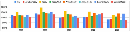
Figure 2.
Percentage profit loss for each forecasting method.
Clearly, the lower , the more accurate the forecast and, as highlighted in Section 6.1, the heuristic average-based methods yield better performance in some years, whereas the econometric methods are better in other periods. Here, we are interested in comparing this result with the prediction given by the standard statistical loss functions, as well as the metrics introduced in Section 4.
Table 4, Table 5, Table 6, Table 7 and Table 8 detail the value of each loss function for each price forecasting method from 2019 through 2023. Within each column, i.e., for each loss function, lower values indicate higher accuracy; however, due to the different nature of the loss functions, a comparison between their respective values is not immediate and will be presented in a more comparable form right after the raw data.
Table 4.
Price forecasting metrics for each method: 2019.
Table 5.
Price forecasting metrics for each method: 2020.
Table 6.
Price forecasting metrics for each method: 2021.
Table 7.
Price forecasting metrics for each method: 2022.
Table 8.
Price forecasting metrics for each method: 2023.
In order to ease the comparison, we further normalized these results by assigning value 1 to the worst-performing metric within each column and rescaling the other values as percentages. For example, if we look at Table 4, we see that according to the MAE loss function, the best performing is the SARIMA Modal (lowest value) and the worst-performing method is Today (highest value). Then, we assigned the value 1 to Today and normalized all other values accordingly.
The results are in Figure 3, Figure 4, Figure 5, Figure 6 and Figure 7, which can be interpreted as follows: for each loss function, the price forecast corresponding to the lowest value is considered the best, and the price forecast corresponding to the highest value (1) is the poorest.
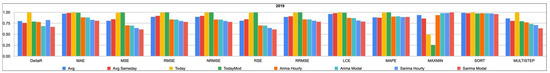
Figure 3.
Relative comparison of price forecasting metrics for each method: 2019.
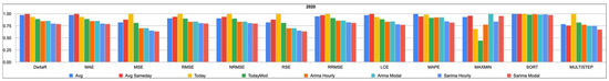
Figure 4.
Relative comparison of price forecasting metrics for each method: 2020.
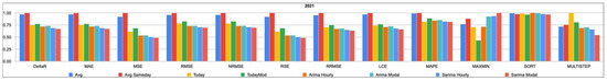
Figure 5.
Relative comparison of price forecasting metrics for each method: 2021.
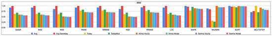
Figure 6.
Relative comparison of price forecasting metrics for each method: 2022.
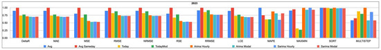
Figure 7.
Relative comparison of price forecasting metrics for each method: 2023.
While in 2019 and 2021 most standard statistical loss functions are able to predict the profit-maximizing strategy, this is no longer true in 2020, 2022, and 2023. Furthermore, the comparison between the histogram of the profit indicator (Figure 2) and those of standard accuracy metrics reveals a lack of qualitative similarity, underscoring the inadequacy of standard metrics in accurately identifying the most profitable forecasting methods for storage operations.
In contrast, our analysis of custom metrics yielded insightful results: the MaxMin metric’s histogram diverges significantly from that of the profit indicator , indicating its unreliability in forecasting the most profitable methods. This finding suggests that merely predicting the highest and lowest price hours under the model assumptions (Section 3) is insufficient for maximizing storage operator profits.
The sort metric’s histogram bears a qualitative resemblance to that of , especially when examining the top-performing models within each category (i.e., Avg and Avg Sameday for heuristic methods and ARIMA Modal and SARIMA Modal for econometric approaches). This implies that accurately sorting hours by energy price can indeed be crucial for optimizing storage operating profits under our model’s assumptions. Similarly, the multistep metric’s histogram captures the trend of the histogram, demonstrating its effectiveness in predicting which forecasting methods will yield higher profits for storage operators. In years 2022 and 2023 the multistep metric is the only one able to capture the high performance of the average-based forecasts.
In addition to the metric’s greater or lower ability to identify the best price-forecasting method when applied to profit maximization, it is also relevant how well each metric estimates the profit loss due to imperfect knowledge of the energy prices. This quality is important in ranking the forecasting methods accurately with respect to profit maximization. To clarify this aspect, for each of the standard and custom metrics (MAE, MSE, multistep, etc.) we computed what the predicted loss of profit would be for each of the forecasting methods (Avg, Avg Sameday, SARIMA Modal, etc.).
Namely, we defined the relative loss value as the percentage of the loss value determined by the metric with respect to the maximum of all loss values. We then compared such value with the percentage loss of profit when applying that forecasting method. Such comparison highlights how well each of the metrics tracks the profit loss. To ease the comparison, we show in Table 9 the deviation of the relative loss value from the exact profit loss, for each metric and forecasting method. A value of 0 for a given metric on a given forecasting method would indicate that that metric is in accordance with the profit loss, predicting it exactly.
Table 9.
Error in profit loss estimation for each metric and method (2019–2023).
For instance, the value corresponding to column MStep and row Avg indicates that the multistep metric predicts the profit lost due to the use of the Avg method (as opposed to perfect knowledge of the future) with an error of . Thus, the lower these values, the more accurate a given metric is at predicting the profit that will be lost due to the use of each forecasting method as opposed to foreseeing the future. The same results are also shown, to enhance readability, in Figure 8, where it is obvious how the MStep error is consistently lower.
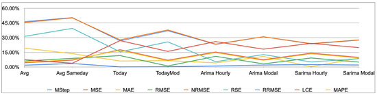
Figure 8.
Error in profit loss estimation for each metric and method (2019–2023).
Figure 9 shows the error in predicting the profit loss for each metric, averaged over all forecasting methods through years 2019–2023. For instance, the error made by the multistep metric in predicting the profit loss due to imperfect knowledge of the future is only , as opposed to an average error of for the MAE metric.
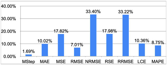
Figure 9.
Error in profit loss estimation for each metric (2019–2023).
But, how is it that the multistep metric is able to track the profit with such accuracy? Going back to its definition in Section 4, the multistep metric effectively simulates the profit by exploiting price differences and realizing an expected profit whenever a higher price is matched with a lower price at a preceding hour during the same day. This does not entirely correspond to the optimal profit-maximizing strategy since the optimal strategy could exploit the higher capacity of the storage system with respect to the energy transferred in a given hour. In other words, the multistep function acts as if the operator were to transfer the entire energy stored each time. Thus, we would expect the real profit to be higher than what predicted by the multistep metric. What is remarkable, though, is that the error in such an approximation is consistently low throughout 2019–2023 and irrespective of the forecasting method employed.
To confirm this intuition, Figure 10 shows the profit loss and the multistep metric averages through the years 2019–2023 for each forecasting method. It is apparent how the multistep metric tracks the profit lost due to forecast with remarkable accuracy while being slightly higher in its estimate due to the limitation highlighted above.
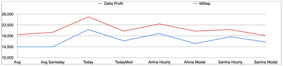
Figure 10.
Profit loss vs. multistep metric averages (2019–2023).
The correlation between the profit lost due to inaccuracy in forecasting energy prices and the multistep metric is even more apparent if we plot the actual profit loss vs. the multistep metric for all forecasting methods in a scatter diagram. Figure 11 displays such a correlation for years 2019–2023.
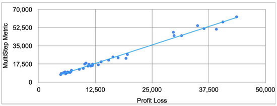
Figure 11.
Profit loss vs. multistep metric (2019–2023).
Our findings indicate that traditional statistical accuracy metrics fall short in capturing the true profit-generating capability of these forecasting methods for storage operations. Furthermore, such standard metrics fail at forecasting the profit lost due to imperfect knowledge of the future evolution of the energy prices. The proposed metric, multistep, on the other hand, appears to perform equally well or better at identifying the best forecast when applied to profit maximization, as well as providing very useful insights into the profit lost due to the approximation.
6.3. Robustness Tests
In this section, we aim to further validate the claim that the multistep metric consistently provides an accurate estimation of the profit lost due to imperfect knowledge of future prices while also performing equally well or better than other standard statistical metrics at selecting the more profitable forecasting methods.
To this end, we performed robustness tests by varying the storage system parameters, the time frame for the simulation, the selection periods of extreme stress and fluctuation in energy prices, and the width of the rolling window used in the price forecasting models.
In regard to the storage energy system configuration, the most important factor influencing profit is the ratio between the capacity of the system, set to 4 MWh in our simulations, and the charging or discharging capacity, which has been set to 1 MWh per hour. These parameters are consistent with existing BESS storage systems and with the literature, as described in Section 6.1. Our results show that increasing or decreasing both parameters proportionally yields no different results, whereas a different ratio could change the profit margin for the operator, since he/she would, for example, benefit from a higher discharge capacity by buying/selling higher quantities when the market conditions are optimal. In the BESS configuration described in Section 6.1, the entire storage systems would need 4 h to be completely charged or discharged. If we set the charge/discharge capacity to 2 MWh/hour, it would instead take 2 h to completely charge or discharge the system, yielding higher profit opportunities. The maximum theoretical profits and the profit achieved with each forecasting method by employing a system with a 2 MWh/hour charge/discharge capacity are presented in Table 10.
Table 10.
Revenue for each forecasting method (nominal values in euro). Charge/discharge = 2 MWh/hour.
If we compare this table with Table 1, we notice how the theoretical maximum profit, as well as the profit achieved by each forecasting method, increases, as expected. However, as further clarified by the following Table 11, the behavior of each forecasting model does not significantly change with respect to the case with 1 MWh/hour charge and discharge capacity (Table 2), although we do observe a slightly lower performance of most models.
Table 11.
Revenue percentage of theoretical maximum for each forecasting method. Charge/discharge = 2 MWh/hour.
The capacity of the multistep metric to accurately select the more profitable forecasting method and properly estimate the profit lost due to imperfect knowledge of the energy prices is highlighted in Table 12 and Figure 12. Table 12 reports the error in predicting the profit loss for each forecasting method (rows) and for each metric (columns). The first column, corresponding to the multistep metric, has generally lower values, indicating higher accuracy in evaluating each method with respect to its capacity to maximize profit. By taking the average over all forecasting methods, Figure 12 provides an even more compact representation of such higher accuracy. Such results are consistent with those presented in Section 6.2 for a storage system with a 1 MWh/hour charge/discharge capacity, hence suggesting that the specific configuration of the storage system does not seem to affect the reliability of the multistep metric.
Table 12.
Error in profit loss estimation for each metric and method (2019–2023). Charge/discharge = 2 MWh/hour.

Figure 12.
Average error in profit loss estimation for each metric (2019–2023). Charge/discharge = 2 MWh/hour.
A different set of robustness tests involves testing the accuracy of the multistep metric during times of stress and extreme fluctuation of the energy prices. We identified four test periods:
- Pre-COVID-19: from 1 January 2019 through 9 March 2020
- COVID-19: from 10 March 2020 through 30 September 2020
- Post-COVID-19: from 1 October 2020 through 31 May 2021
- Gas Crisis: from 1 June 2021 through 14 May 2023
and computed the maximum theoretical profit, the profit achieved by each price forecasting method, and the accuracy of all price metrics in each of these time periods.
The maximum theoretical profits and the profit achieved with each forecasting method in each of these time periods are presented in Table 13.
Table 13.
Revenue for each forecasting method (nominal values in euro).
Table 14 shows the accuracy of each forecasting model with respect to profit maximization. Results do not significantly differ from simulations in Section 6.1 (Table 2).
Table 14.
Revenue percentage of theoretical maximum for each forecasting method.
As to the accuracy of the multistep metric at estimating the potential for profit, results are summarized in Table 15, Table 16, Table 17 and Table 18, which report the error in predicting the profit loss for each forecasting method (rows) and for each metric (columns) in each of the considered stress periods.
Table 15.
Pre-COVID-19: Error in profit loss estimation for each metric and method.
Table 16.
COVID-19: Error in profit loss estimation for each metric and method.
Table 17.
Post-COVID-19: Error in profit loss estimation for each metric and method.
Table 18.
Gas Crisis: Error in profit loss estimation for each metric and method.
Figure 13, Figure 14, Figure 15 and Figure 16 summarize the accuracy of each metric by averaging its performance over all price forecasting methods.
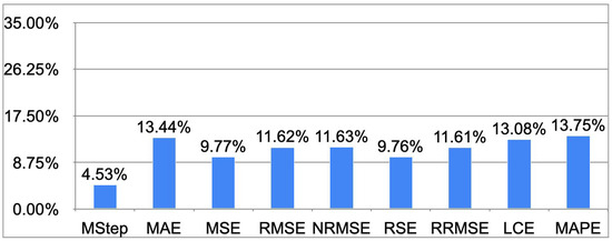
Figure 13.
Pre-COVID-19: Average error in profit loss estimation for each metric.
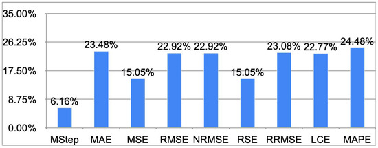
Figure 14.
COVID-19: Average error in profit loss estimation for each metric.
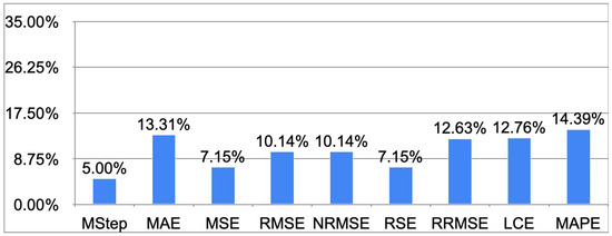
Figure 15.
Post-COVID-19: Average error in profit loss estimation for each metric.

Figure 16.
Gas Crisis: Average error in profit loss estimation for each metric.
Results show that, even in periods of high variability, during which standard statistical metrics fluctuate in their ability to predict the performance of price forecasting methods, the multistep metric is consistently superior, ranging in accuracy from roughly to , whereas standard statistical metrics yield considerably less accurate predictions.
A third robustness test we conducted examines whether the width of the rolling window used in price forecasting methods could impact the efficiency of the multistep metric in accurately predicting profit potential.
Although a detailed analysis of the performance of various price forecasting methods and the optimization of their predictive capabilities is beyond the scope of this work—while it remains a focus of our current research—the width of the rolling windows used was heuristically optimized based on the problem’s characteristics. For instance, following Papaioannou et al. (2016), we observed that a one-year window in ARIMA/SARIMA models captures the seasonal price variations and performs better than narrower windows, while further increasing the data considered does not yield significant improvements in forecasting accuracy. To assess the robustness of the multistep metric, specifically its independence from the chosen time window, we repeated the simulations using each ARIMA/SARIMA model with a rolling window of six months.
Table 19 compares the average efficiency of the methods with the two rolling windows over the period 2019–2023 and shows that results are very similar, with a slight edge of the 12-month window.
Table 19.
ARIMA/SARIMA average efficiency with a 6-month and 12-month rolling window (2019–2023).
Most importantly, the multistep metric remains unaffected by the width of the rolling window in its ability to predict profit. Table 20 shows the deviation in profit loss prediction for each method and metric, while Figure 17 provides a graphical representation of each metric’s predictive capability. The results are consistent with those reported in Table 9 and Figure 8 for a 12-month window.
Table 20.
Error in profit loss estimation with a 6-month rolling window (2019–2023).
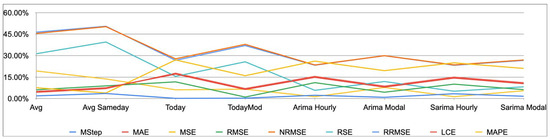
Figure 17.
Error in Profit Loss Estimation for each Metric Using a 6-Months Rolling Window (2019–2023).
Figure 18 highlights the average error in profit prediction for each metric during the period 2019–2023. This result, obtained using a 6-month rolling window, aligns closely with the findings presented in Figure 9 for a 12-month window.

Figure 18.
Average Error in profit loss estimation for each metric using 6-month rolling window (2019–2023).
An analysis using rolling windows of different lengths and varying the amount of data in the heuristic methods Avg and Avg Sameday leads to the same conclusions, demonstrating that the accuracy of the multistep metric is independent of these factors.
7. Conclusions
Due to the evident effects of climate change, the recent evolution of energy markets is more and more oriented towards a progressive reduction in carbon-based electricity production and a parallel progressive substitution by renewable energy sources. As the main part of RESs are not programmable, this substitution tends to destabilize energy markets, determining very low prices in the central hours of sunny and windy days and high prices after the sunset on no-wind days. These price variations do open room for a storage-based trading business, which on the economic side would contribute to a price stabilization and on the technical side would add another power source available when the electric system is short of power. Thus, the storage activity will be crucial for an RES-based electricity market, and in a free market, its economic sustainability is a key factor.
For an energy storage business activity, price prediction accuracy is a critical factor in determining optimal storage policies, with particular emphasis on how price curves influence operational decisions. As this influence is highly nonlinear, a metric capable of proxying the forecasting prices quality for income maximization is a need.
To evaluate the performance of different price forecasting methods, we compared the profits they could generate in the Sardinian electricity market from 2019 to 2023 and assessed their relationship with each method’s statistical accuracy metrics. Interestingly, price forecasting methods that performed better in statistical terms did not necessarily yield higher profits in practice. This suggests that standard accuracy metrics can lack the ability to adequately estimate potential profits.
To address this shortcoming, we developed and tested alternative possible metrics. Our proposed approach moves beyond traditional accuracy benchmarks by quantifying both the predictive power of each model and its practical utility in enhancing storage operations to maximize profitability.
The proposed metric, multistep, outperforms the standard metrics in estimating the potential profit and in identifying the best price forecasting method for an energy storage operator.
Our findings suggest that tracking the exact price curve can be less important than capturing key market features such as price oscillations, intraday sorting, or local extrema, since these are the elements that ultimately guide decisions about whether to buy or sell at a given time.
These results have significant implications, as the availability of a metric specifically suited for proxying the potential profits would greatly simplify the evaluations of the possible profits for different storage technologies and settings and for a more specific tailoring of public subsidy for storage or programmable RES plants. This simplification can thus help in planning the road towards a higher share of RESs, a reduction in carbon emissions, and more sustainable energy production.
Author Contributions
S.S.: Conceptualization, Methodology, Software, Validation, Formal Analysis, Investigation, Data Curation, Writing—original draft, Writing—review & editing, Visualization. A.F.M.: Conceptualization, Methodology, Software, Validation, Formal Analysis, Investigation, Data Curation, Writing—original draft, Writing—review & editing, Visualization. S.Z.: Conceptualization, Methodology, Validation, Investigation, Writing—original draft, Writing—review & editing, Visualization, Supervision, Project administration, Funding Acquisition. All authors have read and agreed to the published version of the manuscript.
Funding
This study received funding from the European Union-Next-GenerationEU-National Recovery and Resilience Plan (NRRP)–MISSION 4 COMPONENT 2, INVESTMENT N. 1.1, CALL PRIN 2022 PNRR D.D. 1409 14-09-2022–Incorporating climate-related risks into financial stability assessments: where are we now and how can we move forward? CUP N. P2022WM82K.
Data Availability Statement
The datasets generated and/or analyzed during the study are available from the authors on reasonable request.
Conflicts of Interest
The authors declare no conflicts of interest.
Appendix A. Standard Loss Functions
For the reader’s convenience, we summarize here the standard statistical loss functions used in this paper. For further information, please refer to Jadon et al. (2024).
The Mean Absolute Error (MAE) loss functions represents the arithmetic mean of absolute errors
The Mean Squared Error (MSE) squares the difference between the predicted value and actual value and averages it across the dataset
The Root Mean Squared Error (RMSE) is defined as:
The Normalized Root Mean Squared Error (NRMSE) is normalized with the mean of the correct price values
where .
The Relative Squared Error (RSE) is obtained by dividing the MSE of our model by the MSE of a model which uses the mean of the predicted value
with . The Relative Root Mean Squared Error (RRMSE) is a variant of Root Mean Squared Error (RMSE), gauging predictive model accuracy relative to the target variable range
The Log Cosh Error (LCE) calculates the logarithm of the hyperbolic cosine of the error
The Mean Absolute Percentage Error (MAPE)1 is a relative error measure that uses absolute values to keep the positive and negative errors from canceling one another out and is defined as
Appendix B. Forecasting the Evolution of the Energy Prices
The discrete-time storage evolution model is inherently stochastic because the future evolution of energy prices is unknown. To evaluate any specific strategy, we must assume a particular trajectory for the price curve. One approach involves generating random scenarios based on a price evolution model or by introducing random variations to a given price forecast. While these methods can yield valuable insights, it is equally important to test forecasting strategies commonly used by industry practitioners. For instance, energy operators often predict that short-term prices will remain relatively stable or that their near-term behavior will resemble the average of the past K days. Accordingly, we have incorporated several forecasting techniques, as suggested by operators, into our simulation software. Their performance has been thoroughly studied and compared in Sbaraglia et al. (2024).
Appendix B.1. Econometric Price Forecasting Methods
The econometric methods that we considered are based on a selection process of the appropriate ARIMA and SARIMA models, driven by the Akaike Information Criterion (AIC). Specifically, we independently evaluated the time series data for each hour to determine the optimal model parameters for ARIMA and for SARIMA that minimized the AIC score. This involved considering all combinations of these parameters, with values ranging from zero to seven. This analysis segmented the hourly price data from 2018 to 2023 into 24 distinct time series, one for each hour of the day. For each time series, corresponding to a specific hour, the best-fitting ARIMA/SARIMA models were determined for each year.
The ARIMA orders for the “ARIMA Hourly” method, shown in Table A1, were selected using the Akaike Information Criterion, evaluating all possible configurations ( ranging from 0 to 7) based on their fit to historical prices for the same hour in the previous year. For the “ARIMA Modal” method, the modal value among these best configurations across the 24 h was used.
Table A1.
ARIMA orders used for the “SARIMA Hourly” method.
Table A1.
ARIMA orders used for the “SARIMA Hourly” method.
| Hour | 2019 | 2020 | 2021 | 2022 | 2023 |
|---|---|---|---|---|---|
| 1 | (2, 1, 1) | (1, 1, 1) | (1, 1, 1) | (1, 1, 1) | (0, 1, 2) |
| 2 | (2, 1, 1) | (1, 1, 1) | (1, 1, 1) | (2, 1, 2) | (0, 1, 1) |
| 3 | (1, 1, 1) | (1, 1, 1) | (1, 1, 1) | (1, 1, 1) | (1, 1, 2) |
| 4 | (1, 1, 1) | (1, 1, 1) | (5, 1, 1) | (1, 1, 1) | (1, 1, 1) |
| 5 | (1, 1, 1) | (1, 1, 1) | (1, 1, 1) | (1, 1, 1) | (1, 1, 1) |
| 6 | (1, 1, 1) | (1, 1, 1) | (1, 1, 1) | (3, 1, 5) | (1, 1, 1) |
| 7 | (1, 1, 1) | (1, 1, 1) | (1, 1, 1) | (1, 1, 1) | (1, 1, 1) |
| 8 | (0, 1, 2) | (6, 1, 5) | (7, 1, 6) | (2, 1, 2) | (0, 1, 2) |
| 9 | (0, 1, 2) | (2, 1, 1) | (7, 1, 0) | (6, 1, 5) | (3, 1, 3) |
| 10 | (2, 1, 1) | (0, 1, 2) | (6, 1, 0) | (5, 1, 2) | (1, 1, 1) |
| 11 | (0, 1, 1) | (1, 1, 1) | (1, 1, 1) | (3, 1, 1) | (1, 1, 1) |
| 12 | (2, 1, 1) | (1, 1, 1) | (0, 1, 2) | (3, 1, 1) | (1, 0, 1) |
| 13 | (7, 1, 5) | (1, 1, 1) | (1, 1, 2) | (1, 1, 1) | (1, 0, 1) |
| 14 | (1, 1, 1) | (1, 1, 1) | (0, 1, 1) | (1, 1, 1) | (2, 0, 1) |
| 15 | (1, 1, 1) | (3, 0, 1) | (0, 1, 2) | (1, 1, 1) | (1, 0, 1) |
| 16 | (1, 1, 1) | (2, 1, 1) | (7, 1, 0) | (1, 1, 1) | (1, 0, 1) |
| 17 | (1, 1, 1) | (0, 1, 2) | (1, 1, 1) | (1, 1, 1) | (2, 1, 2) |
| 18 | (5, 1, 3) | (1, 1, 1) | (3, 1, 1) | (1, 1, 1) | (1, 1, 1) |
| 19 | (1, 1, 2) | (1, 1, 1) | (3, 1, 1) | (1, 1, 1) | (1, 1, 1) |
| 20 | (0, 1, 1) | (1, 1, 1) | (1, 1, 1) | (2, 1, 1) | (3, 1, 3) |
| 21 | (0, 1, 1) | (1, 1, 1) | (1, 1, 1) | (3, 1, 2) | (0, 1, 2) |
| 22 | (1, 1, 3) | (1, 1, 1) | (1, 1, 1) | (1, 1, 0) | (0, 1, 2) |
| 23 | (3, 1, 4) | (1, 1, 2) | (1, 1, 1) | (0, 1, 1) | (0, 1, 2) |
| 24 | (0, 1, 2) | (1, 1, 1) | (1, 1, 1) | (1, 1, 0) | (4, 1, 1) |
The SARIMA orders for the “SARIMA Hourly” method, shown in Table A2, were selected using the Akaike Information Criterion, evaluating all possible configurations ( ranging from 0 to 7) based on their fit to historical prices for the same hour in the previous year, with the seasonal parameter s fixed at 7 to account for weekly seasonality. For the “SARIMA Modal” method, the modal value among the best feasible configurations across the 24 h was used.
Once the optimal models were identified through this process, we designed two distinct forecasting approaches:
ARIMA Hourly/SARIMA Hourly: Employing a “multi-set” strategy, we forecasted hourly prices for each year (from 2019 to 2023) using the best model parameters identified for that specific hour in the preceding year. This method ensured that the unique daily price fluctuations were appropriately captured by using distinct models for each hour.
ARIMA Modal/SARIMA Modal: This “one-set” approach involved forecasting hourly prices using a single set of model parameters, consisting of the modal (most frequently optimal) parameters among the 24 hourly models from the previous year. This method aims for generality across all hours by taking advantage of the most common set of optimal parameters.
For each of the ARIMA and SARIMA models, the parameter selection is based on the Akaike Information Criterion (AIC), ensuring a rigorous comparison of various configurations. In the AIC optimization criterion, each time series for each specific hour of the day is considered independently and the best parameters for that specific hour forecast are obtained. Then we proceeded by employing these best-fit parameters in two manners: in the ARIMA/SARIMA one-set approach a single set of parameters is chosen, as being the best performing set of the majority of hourly time series. This single set is then used to simulate the prices for all hours of the day. In the second, ARIMA/SARIMA multi-set approach, we have employed the best set of parameters for each hour of the day, thus utilizing different ARIMA/SARIMA models to predict the prices at different hours in order to take account for specific daily variations in the price characteristics.
Table A2.
SARIMA orders used for the “SARIMA Hourly” method.
Table A2.
SARIMA orders used for the “SARIMA Hourly” method.
| Hour | 2019 | 2020 | 2021 | 2022 | 2023 |
|---|---|---|---|---|---|
| 1 | (2,1,1) (1,0,1) | (1,1,2) (1,0,1) | (1,1,1) (1,0,0) | (0,1,2) (2,0,2) | (0,1,2) (0,0,0) |
| 2 | (2,1,1) (2,0,0) | (1,1,2) (1,0,1) | (1,1,1) (0,0,0) | (0,1,2) (1,0,1) | (0,1,1) (0,0,0) |
| 3 | (1,1,1) (0,0,2) | (1,1,2) (1,0,1) | (1,1,1) (0,0,0) | (0,1,1) (1,0,1) | (1,1,2) (0,0,0) |
| 4 | (1,1,1) (1,0,1) | (1,1,2) (1,0,1) | (1,1,2) (1,0,1) | (2,1,1) (1,0,1) | (1,1,1) (0,0,0) |
| 5 | (1,1,1) (1,0,1) | (1,1,1) (0,0,0) | (1,1,1) (1,0,0) | (1,1,3) (1,0,1) | (1,1,1) (0,0,0) |
| 6 | (1,1,1) (1,0,0) | (1,1,1) (0,0,0) | (1,1,1) (1,0,0) | (1,1,1) (1,0,1) | (1,1,1) (0,0,0) |
| 7 | (3,1,1) (1,0,1) | (1,1,1) (1,0,2) | (1,1,1) (0,0,2) | (4,1,0) (1,0,1) | (1,1,2) (1,0,0) |
| 8 | (1,1,1) (1,0,2) | (1,1,1) (0,0,2) | (1,1,1) (1,0,2) | (4,1,0) (1,0,1) | (0,1,2) (0,0,2) |
| 9 | (1,1,3) (1,0,2) | (0,1,3) (0,0,2) | (1,1,2) (1,0,2) | (3,1,0) (1,0,1) | (1,1,2) (2,0,0) |
| 10 | (0,1,3) (0,0,2) | (1,1,1) (1,0,2) | (1,1,1) (1,0,1) | (3,1,2) (1,0,1) | (1,1,1) (0,0,2) |
| 11 | (0,1,1) (0,0,2) | (2,1,1) (2,0,1) | (1,1,1) (0,0,2) | (2,1,1) (1,0,1) | (1,1,1) (1,0,0) |
| 12 | (0,1,1) (1,0,1) | (2,1,1) (2,0,2) | (1,1,1) (0,0,2) | (2,1,1) (1,0,1) | (2,0,0) (1,0,1) |
| 13 | (1,1,2) (2,0,2) | (2,1,1) (2,0,2) | (1,1,1) (1,0,0) | (1,1,2) (1,0,1) | (1,0,1) (2,0,1) |
| 14 | (2,1,1) (1,0,2) | (1,1,1) (2,0,2) | (0,1,1) (0,0,0) | (1,1,2) (1,0,1) | (2,0,0) (1,0,1) |
| 15 | (4,1,1) (2,0,1) | (2,0,0) (1,0,2) | (1,1,1) (0,0,2) | (1,1,2) (1,0,1) | (2,0,0) (1,0,1) |
| 16 | (1,1,1) (2,0,1) | (1,1,1) (1,0,1) | (1,1,1) (1,0,2) | (2,1,1) (1,0,1) | (1,0,1) (1,0,1) |
| 17 | (1,1,1) (0,0,2) | (1,1,2) (2,0,1) | (1,1,1) (0,0,2) | (1,1,2) (1,0,2) | (1,1,1) (1,0,0) |
| 18 | (2,1,1) (1,0,1) | (1,1,3) (2,0,1) | (1,1,1) (1,0,1) | (1,1,2) (1,0,1) | (1,1,1) (0,0,0) |
| 19 | (2,1,1) (1,0,1) | (1,1,2) (1,0,1) | (1,1,1) (1,0,1) | (2,1,1) (1,0,1) | (1,1,1) (1,0,0) |
| 20 | (0,1,1) (2,0,1) | (1,1,1) (1,0,0) | (1,1,1) (1,0,1) | (1,1,2) (1,0,1) | (3,1,2) (1,0,1) |
| 21 | (0,1,1) (2,0,0) | (1,1,2) (0,0,1) | (1,1,1) (1,0,1) | (3,1,2) (2,0,0) | (0,1,2) (0,0,0) |
| 22 | (1,1,3) (0,0,0) | (1,1,1) (2,0,1) | (1,1,1) (1,0,1) | (1,1,0) (1,0,1) | (0,1,2) (0,0,0) |
| 23 | (1,1,2) (2,0,2) | (1,1,2) (0,0,1) | (2,1,1) (1,0,1) | (0,1,1) (0,0,0) | (0,1,2) (0,0,0) |
| 24 | (1,1,1) (1,0,1) | (1,1,1) (0,0,1) | (1,1,1) (1,0,1) | (1,1,0) (0,0,0) | (4,1,1) (0,0,0) |
The ARIMA and SARIMA models were applied using a rolling window approach, a technique particularly effective for time series forecasting in dynamic environments like electricity pricing. This method involves continuously updating the dataset used for model training, ensuring that the most recent data is always included. Specifically, for each new forecast, the model is retrained on a shifted dataset window that encompasses the latest 30 days of data, effectively ‘rolling’ the window forward with each new prediction. For example, to forecast the electricity price at a given hour of 2 January 2019, the model uses data of prices (for the same hour) from 3 December 2018, to 1 January 2019. As we move to January 3, the window shifts to include data from 4 December 2018, to 2 January 2019, and so on.
Appendix B.2. Heuristic Price Forecasting Methods
The following four additional forecasting models have been adopted in order to offer an alternative simple, heuristic, and operator-driven approach to predicting electricity prices:
- Today Model: This model is straightforward, predicting that the electricity price at any given hour will be the same as it was at the same hour the previous day. It is a simple approach that assumes day-to-day price stability.
- Today_mod Model: This model adds a layer of specificity to the Today model by partially accounting for weekly patterns. For Saturdays, Sundays, and Mondays, the “Today_mod” model predicts that electricity prices at each specific hour will be the same as those observed at the same specific hour on the preceding week’s corresponding day (Saturday, Sunday, or Monday). For Tuesdays, Wednesdays, Thursdays, and Fridays, the model predicts that electricity prices at each specific hour will be the same as those observed at the same hour on the immediately preceding day. This approach combines the simplicity of the “Today” model with a more nuanced understanding of potential weekly patterns, particularly for weekends and the start of the week.
- Average Model: By averaging the electricity prices of the same hour over the past 30 days, this model seeks to smooth out short-term fluctuations and capture a more stable, long-term trend. This method could be effective in dampening the impact of anomalous price spikes or drops.
- Average_same_day Model: This model focuses on the weekly cycle, averaging the prices of the same hour on the same weekday over the past four weeks. It is a nuanced approach that recognizes potential weekly cycles, similar to the Today_mod model but with a broader historical perspective.
A more in-depth treatment of the price forecasting methods, as well as a rigorous study of the best coupling of each price forecasting method with the optimal operator strategy, can be found in Sbaraglia et al. (2024).
Note
| 1 | Although MAPE is a widespread and generally insightful loss function, it is worth noting that it might become undefined or excessively skewed when dealing with zero or near-zero values, as the percentage error calculation involves division by the actual value. This characteristic makes MAPE less reliable in the context of energy markets where price fluctuations can include such scenarios, as it is the one considered in our paper. |
References
- Acaroğlu, Hakan, and Fausto Pedro García Márquez. 2021. Comprehensive review on electricity market price and load forecasting based on wind energy. Energies 14: 7473. [Google Scholar] [CrossRef]
- Agathokleous, Rafaela A., Giovanni Barone, Annamaria Buonomano, Cesare Forzano, Soteris A. Kalogirou, and Adolfo Palombo. 2019. Building façade integrated solar thermal collectors for air heating: Experimentation, modelling and applications. Applied Energy 239: 658–79. [Google Scholar] [CrossRef]
- Alkawaz, Ali Najem, Abdallah Abdellatif, Jeevan Kanesan, Anis Salwa Mohd Khairuddin, and Hassan Muwafaq Gheni. 2022. Day-ahead electricity price forecasting based on hybrid regression model. IEEE Access 10: 108021–33. [Google Scholar] [CrossRef]
- Antweiler, Werner. 2021. Microeconomic models of electricity storage: Price Forecasting, arbitrage limits, curtailment insurance, and transmission line utilization. Energy Economics 101: 105390. [Google Scholar] [CrossRef]
- Babu, C. Narendra, and B. Eswara Reddy. 2014. A moving-average filter based hybrid ARIMA–ANN model for forecasting time series data. Applied Soft Computing 23: 27–38. [Google Scholar] [CrossRef]
- Beigaite, Rita, Tomas Krilavičius, and Ka Lok Man. 2018. Electricity price forecasting for nord pool data. Paper presented at International Conference on Platform Technology and Service (PlatCon), Jeju, Republic of Korea, January 29–31. [Google Scholar]
- Belenguer, Enrique, Jorge Segarra-Tamarit, Emilio Pérez, and Ricardo Vidal-Albalate. 2025. Short-term electricity price forecasting through demand and renewable generation prediction. Mathematics and Computers in Simulation 229: 350–61. [Google Scholar] [CrossRef]
- Bissing, Daniel, Michael T. Klein, Radhakrishnan Angamuthu Chinnathambi, Daisy Flora Selvaraj, and Prakash Ranganathan. 2019. A Hybrid Regression Model for Day-Ahead Energy Price Forecasting. IEEE Access 7: 36833–42. [Google Scholar] [CrossRef]
- Cerjan, Marin, Ivana Krzelj, Marko Vidak, and Marko Delimar. 2013. A literature review with statistical analysis of electricity price forecasting methods. Paper presented at Eurocon 2013, Zagreb, Croatia, July 1–4; pp. 756–63. [Google Scholar] [CrossRef]
- Chaâbane, Najeh. 2014. A hybrid ARFIMA and neural network model for electricity price prediction. International Journal of Electrical Power & Energy Systems 55: 187–94. [Google Scholar]
- Connolly, David, Henrik Lund, Paddy Finn, Brian Vad Mathiesen, and Martin Leahy. 2011. Practical operation strategies for pumped hydroelectric energy storage (PHES) utilizing electricity price arbitrage. Energy Policy 39: 4189–96. [Google Scholar] [CrossRef]
- De Marcos, Rodrigo A., Antonio Bello, and Javier Reneses. 2019. Electricity price forecasting in the short term hybridising fundamental and econometric modelling. Electric Power Systems Research 167: 240–51. [Google Scholar] [CrossRef]
- Fezzi, Carlo, and Luca Mosetti. 2020. Size matters: Estimation sample length and electricity price forecasting accuracy. The Energy Journal 41: 231–54. [Google Scholar] [CrossRef]
- Ghasemi, Ahmad, Houman Jamshidi Monfared, Abdolah Loni, and Mousa Marzband. 2021. CVaR-based retail electricity pricing in day-ahead scheduling of microgrids. Energy 227: 120529. [Google Scholar] [CrossRef]
- Gunduz, Salih, Umut Ugurlu, and Ilkay Oksuz. 2023. Transfer learning for electricity price forecasting. Sustainable Energy, Grids and Networks 34: 100996. [Google Scholar] [CrossRef]
- Jadon, Aryan, Avinash Patil, and Shruti Jadon. 2024. A comprehensive survey of regression-based loss functions for time series forecasting. In International Conference on Data Management, Analytics & Innovation. Singapore: Springer Nature. [Google Scholar]
- Jędrzejewski, Arkadiusz, Jesus Lago, Grzegorz Marcjasz, and Rafał Weron. 2022. Electricity price forecasting: The dawn of machine learning. IEEE Power and Energy Magazine 20: 24–31. [Google Scholar] [CrossRef]
- Jiang, He, Yawei Dong, Yao Dong, and Jianzhou Wang. 2025. Probabilistic electricity price forecasting by integrating interpretable model. Technological Forecasting and Social Chang 210: 123846. [Google Scholar] [CrossRef]
- Kapoor, Gaurav, and Nuttanan Wichitaksorn. 2023. Electricity price forecasting in New Zealand: A comparative analysis of statistical and machine learning models with feature selection. Applied Energy 347: 121446. [Google Scholar] [CrossRef]
- Kiesel, Rüdiger, and Florentina Paraschiv. 2017. Econometric analysis of 15-minute intraday electricity prices. Energy Economics 64: 77–90. [Google Scholar] [CrossRef]
- Lago, Jesus, Grzegorz Marcjasz, Bart De Schutter, and Rafał Weron. 2021. Forecasting day-ahead electricity prices: A review of state-of-the-art algorithms, best practices and an open-access benchmark. Applied Energy 293: 116983. [Google Scholar] [CrossRef]
- Li, Audeliano Wolian, and Guilherme Sousa Bastos. 2020. Stock market forecasting using deep learning and technical analysis: A systematic review. IEEE Access 8: 185232–42. [Google Scholar] [CrossRef]
- Lu, Hongfang, Xin Ma, Minda Ma, and Senlin Zhu. 2021. Energy price prediction using data-driven models: A decade review. Computer Science Review Volume 39: 100356. [Google Scholar] [CrossRef]
- Makridaki, Spyros, Evangelos Spiliotis, and Vassilios Assimakopoulos. 2018. Statistical and Machine Learning forecasting methods: Concerns and ways forward. PLoS ONE 13: E0194889. [Google Scholar] [CrossRef]
- Mayer, Klaus, and Stefan Trück. 2018. Electricity markets around the world. Journal of Commodity Markets 9: 77–100. [Google Scholar] [CrossRef]
- Mercier, Thomas, Mathieu Olivier, and Emmanuel De Jaeger. 2023. The value of electricity storage arbitrage on day-ahead markets across Europe. Energy Economics 123: 106721. [Google Scholar] [CrossRef]
- Münderlein, Jeanette, Marc Steinhoff, Sebastian Zurmühlen, and Dirk Uwe Sauer. 2019. Analysis and evaluation of operations strategies based on a large scale 5 MW and 5 MWh battery storage system. Journal of Energy Storage 24: 100778. [Google Scholar] [CrossRef]
- Nowotarski, Jakub, and Rafał Weron. 2018. Recent advances in electricity price forecasting: A review of probabilistic forecasting. Renewable and Sustainable Energy Reviews 81: 1548–68. [Google Scholar] [CrossRef]
- Panigrahi, Sibarama, and Himansu Sekhar Behera. 2017. A hybrid ETS-ANN model for time series forecasting. Engineering Applications of Artificial Intelligence 66: 49–59. [Google Scholar] [CrossRef]
- Papaioannou, George P., Christos Dikaiakos, Anargyros Dramountanis, and Panagiotis G. Papaioannou. 2016. Analysis and modeling for short-to medium-term load forecasting using a hybrid manifold learning principal component model and comparison with classical statistical models (SARIMAX, Exponential Smoothing) and artificial intelligence models (ANN, SVM): The case of Greek electricity market. Energies 9: 635. [Google Scholar] [CrossRef]
- Parmezan, Antonio, Vinicius Souza, and Gustavo Batista. 2019. Evaluation of statistical and machine learning models for time series prediction: Identifying the state-of-the-art and the best conditions for the use of each model. Information Sciences 484: 302–37. [Google Scholar] [CrossRef]
- Rafiei, Mehdi, Taher Niknam, and Mohammad Hassan Khooban. 2016. A novel intelligent strategy for probabilistic electricity price forecasting: Wavelet neural network based modified dolphin optimization algorithm. Journal of Intelligent & Fuzzy Systems 31: 301–12. [Google Scholar]
- Sbaraglia, Simone, Alessandro Fiori Maccioni, Emilio Ghiani, and Stefano Zedda. 2024. Is Storage a Business? A Test on the Italian Day-Ahead Electricity Market (February 02, 2024). Available online: https://ssrn.com/abstract=4980380 (accessed on 1 November 2024).
- Shen, Zhipeng, Yuanming Zhang, Jiawei Lu, Jun Xu, and Gang Xiao. 2019. A novel time series forecasting model with deep learning. Neurocomputing 396: 302–13. [Google Scholar] [CrossRef]
- Tibshirani, Robert. 1996. Regression shrinkage and selection via the lasso. Journal of the Royal Statistical Society Series B: Statistical Methodology 58: 267–88. [Google Scholar] [CrossRef]
- Uniejewski, Bartosz, Grzegorz Marcjasz, and Rafał Weron. 2019. Understanding intraday electricity markets: Variable selection and very short-term price forecasting using LASSO. International Journal of Forecasting 35: 1533–47. [Google Scholar] [CrossRef]
- Ugurlu, Umut, Ilkay Oksuz, and Oktay Tas. 2018. Electricity price forecasting using recurrent neural networks. Energies 11: 1255. [Google Scholar] [CrossRef]
- Weron, Rafał. 2014. Electricity price forecasting: A review of the state-of-the-art with a look into the future. International Journal of Forecasting 81: 1548–68. [Google Scholar] [CrossRef]
- Yu, Nanpeng, and Brandon Foggo. 2017. Stochastic valuation of energy storage in wholesale power markets. Energy Economics 64: 177–85. [Google Scholar] [CrossRef]
- Zema, Tomasz, and Adam Sulich. 2022. Models of electricity price forecasting: Bibliometric research. Energies 15: 5642. [Google Scholar] [CrossRef]
- Zhang, G. Peter. 2003. Time series forecasting using a hybrid ARIMA and neural network model. Neurocomputing 50: 159–75. [Google Scholar] [CrossRef]
- Ziel, Florian, and Rick Steinert. 2018. Probabilistic mid-and long-term electricity price forecasting. Renewable and Sustainable Energy Reviews 94: 251–66. [Google Scholar] [CrossRef]
- Zou, Hui, and Yuhong Yang. 2004. Combining time series models for forecasting. International Journal of Forecasting 20: 69–84. [Google Scholar] [CrossRef]


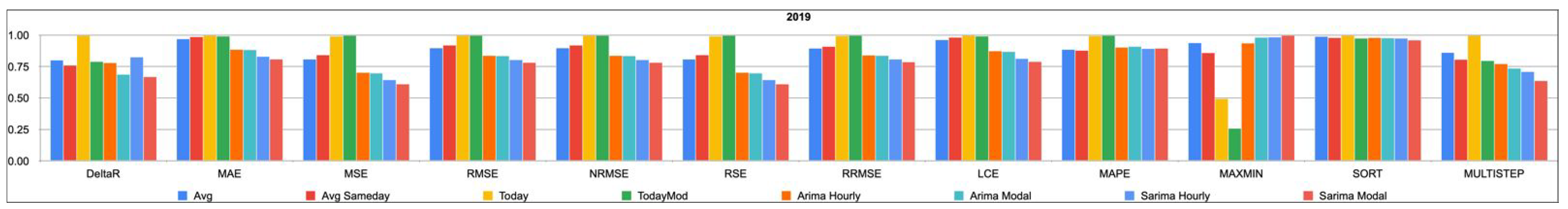
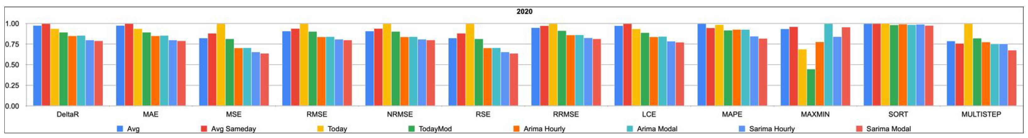
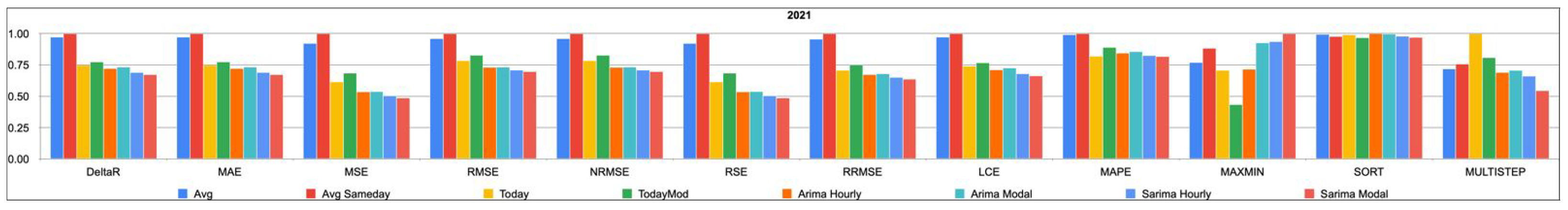
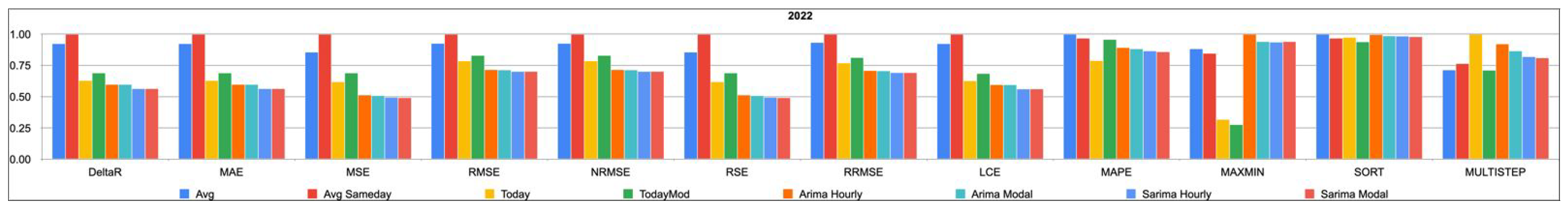
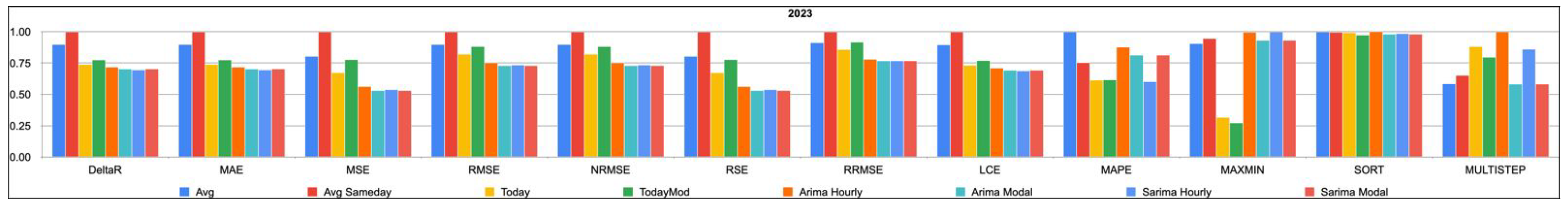
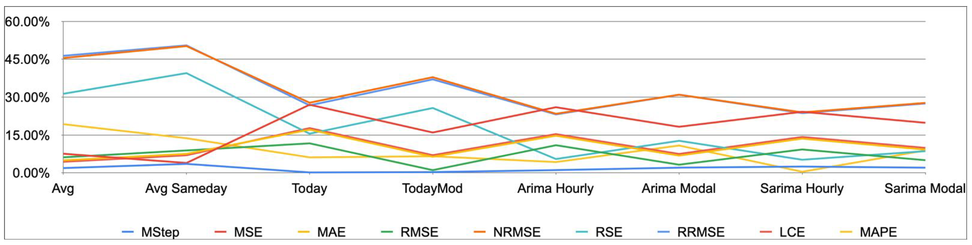
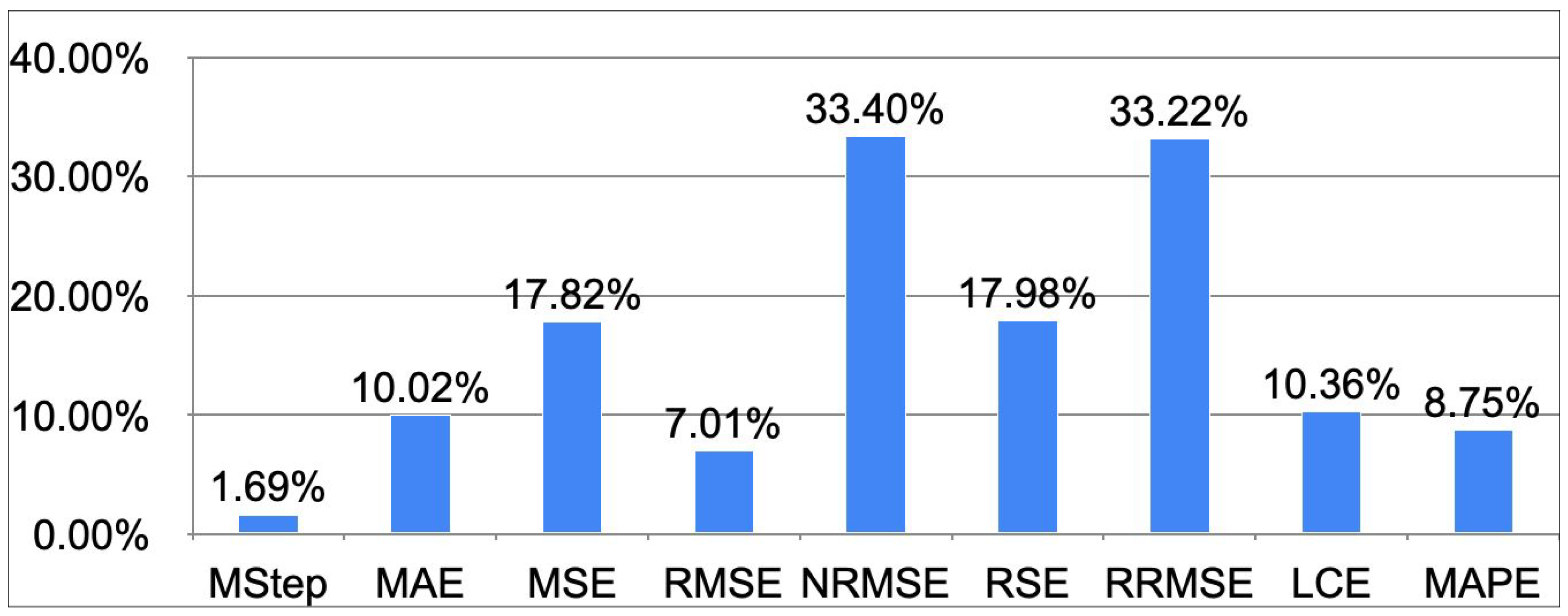
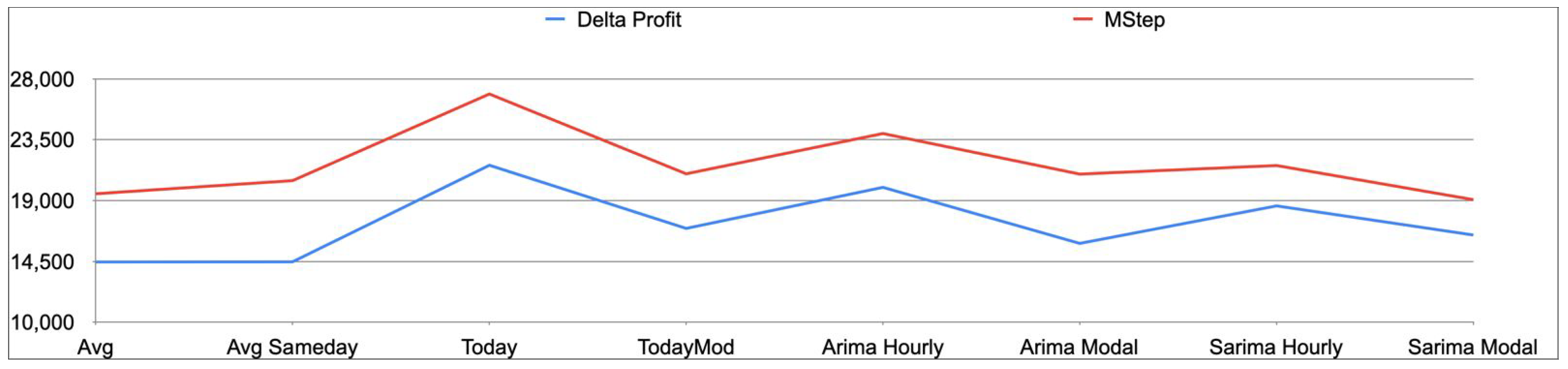
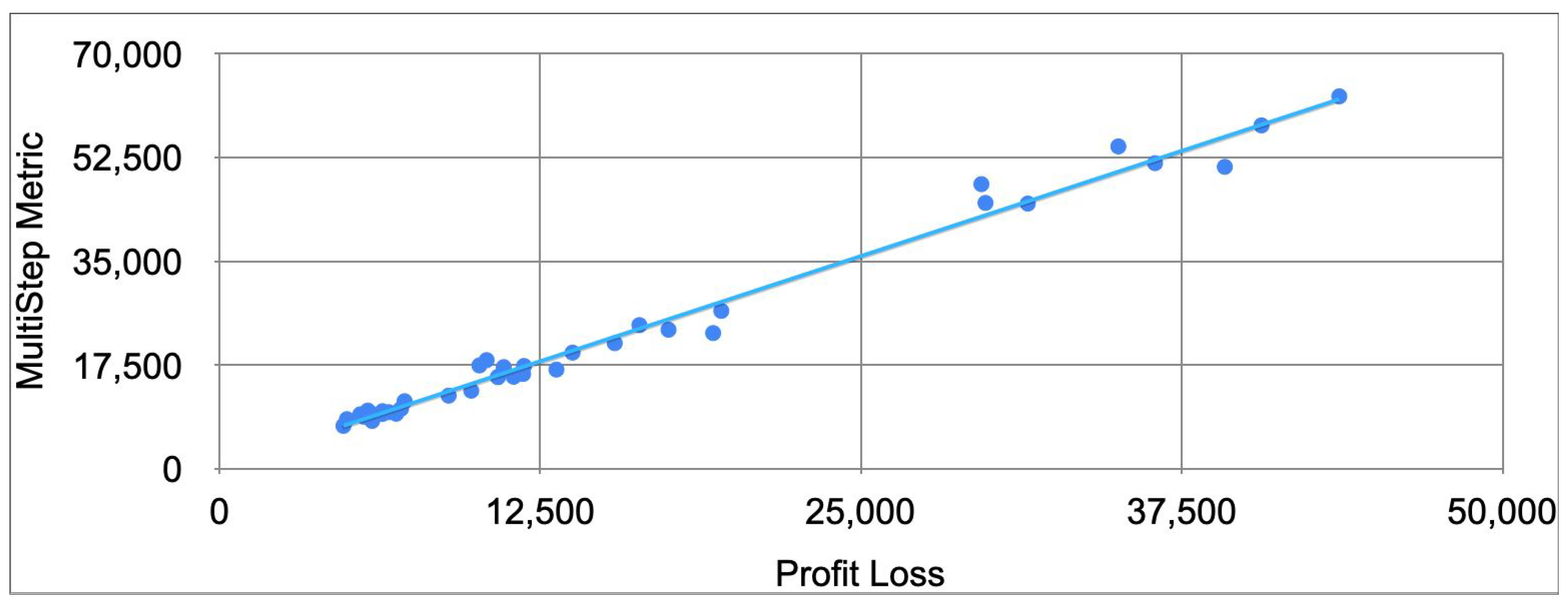
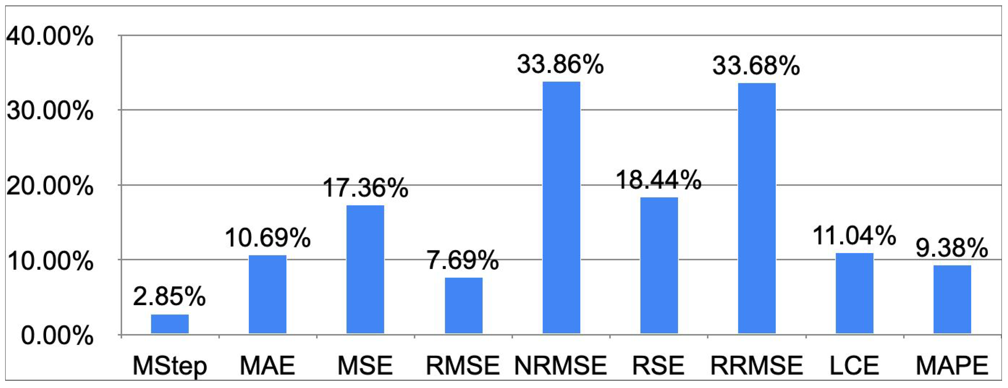
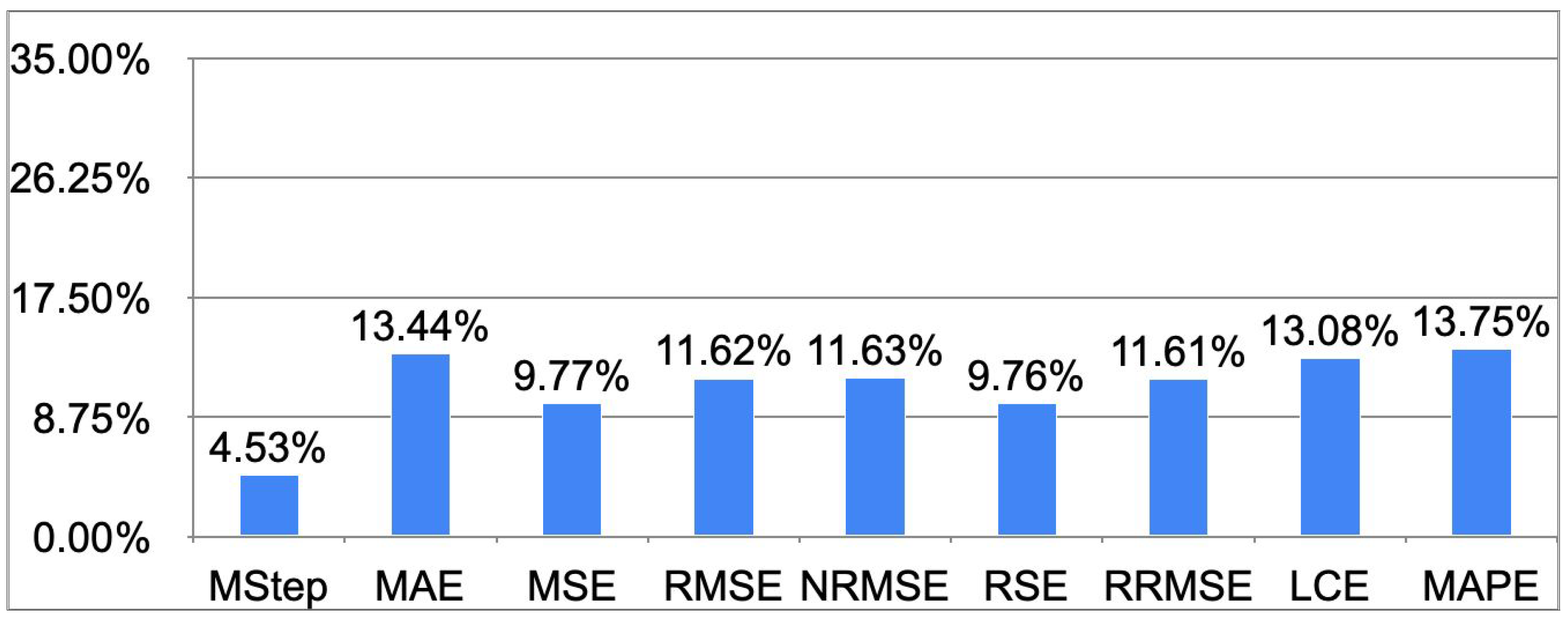
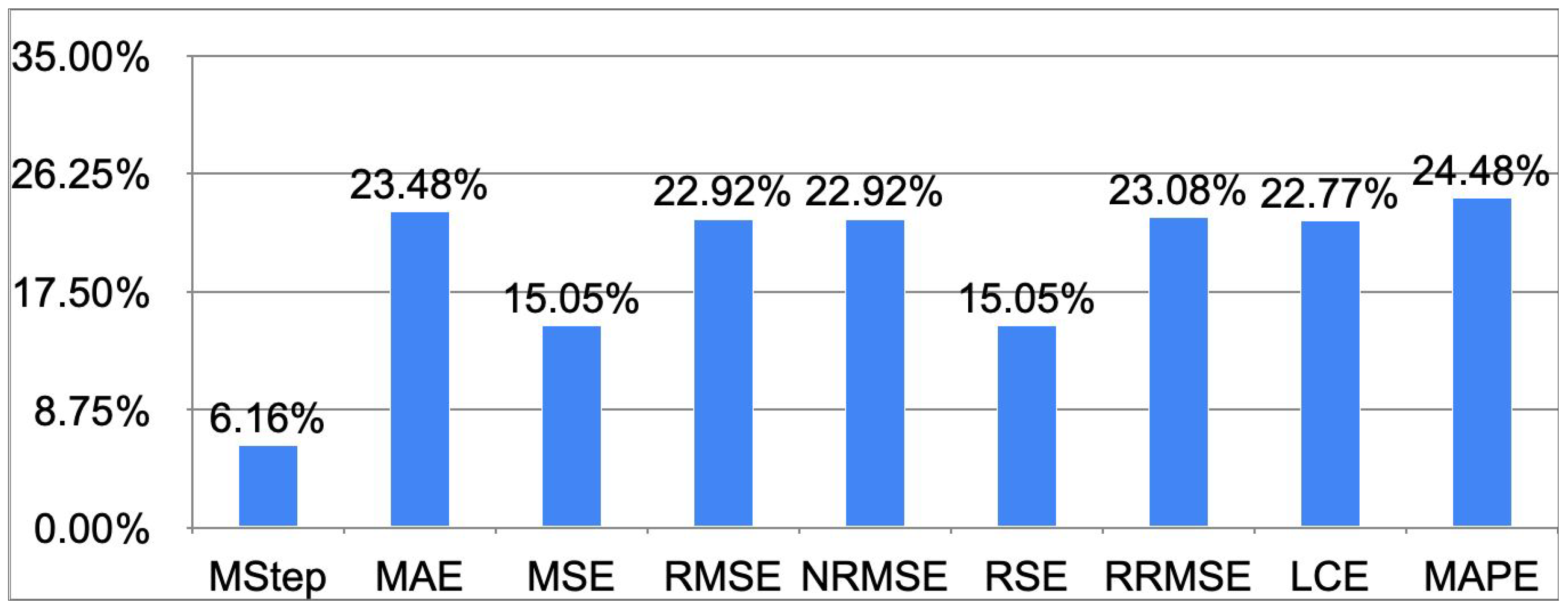
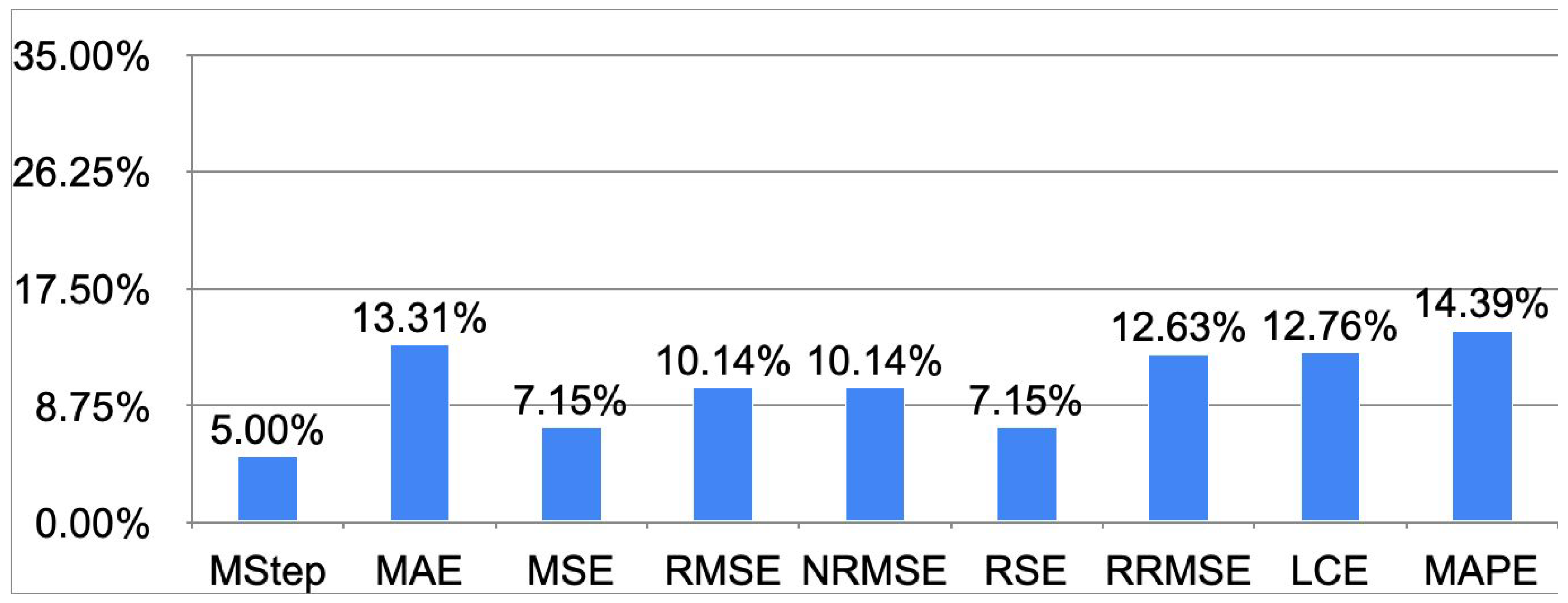
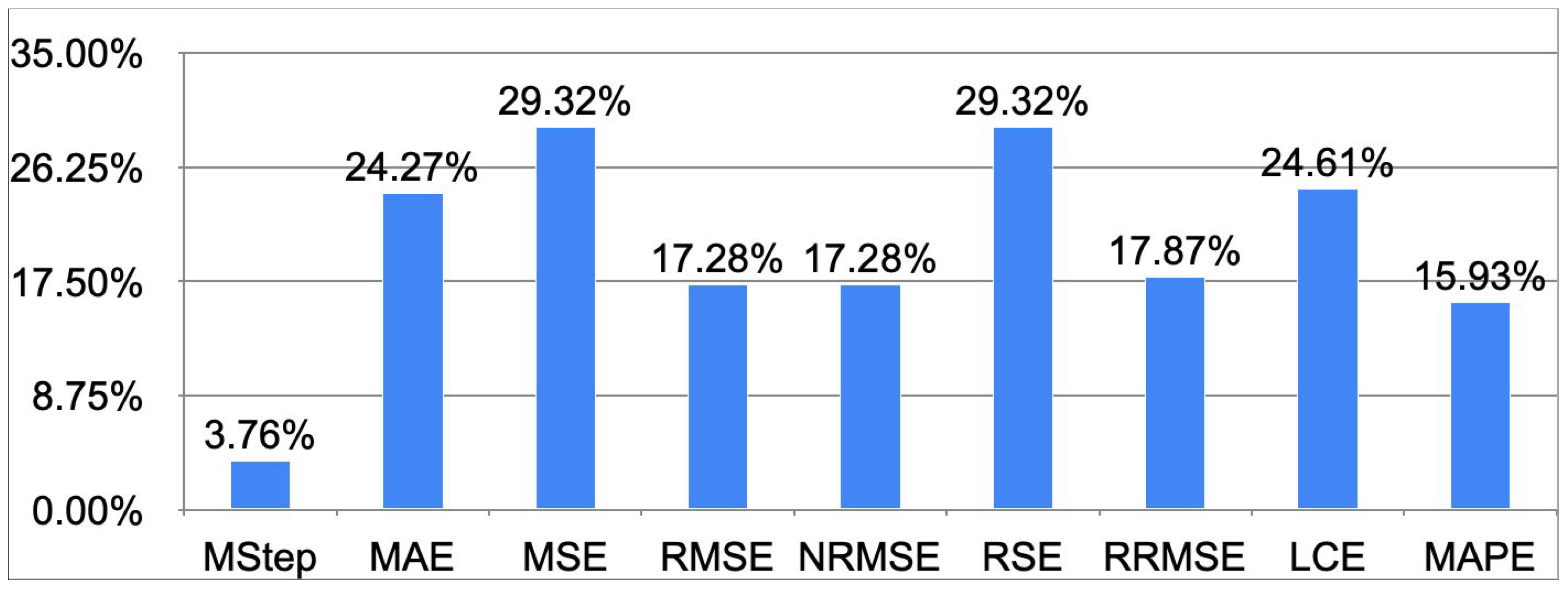
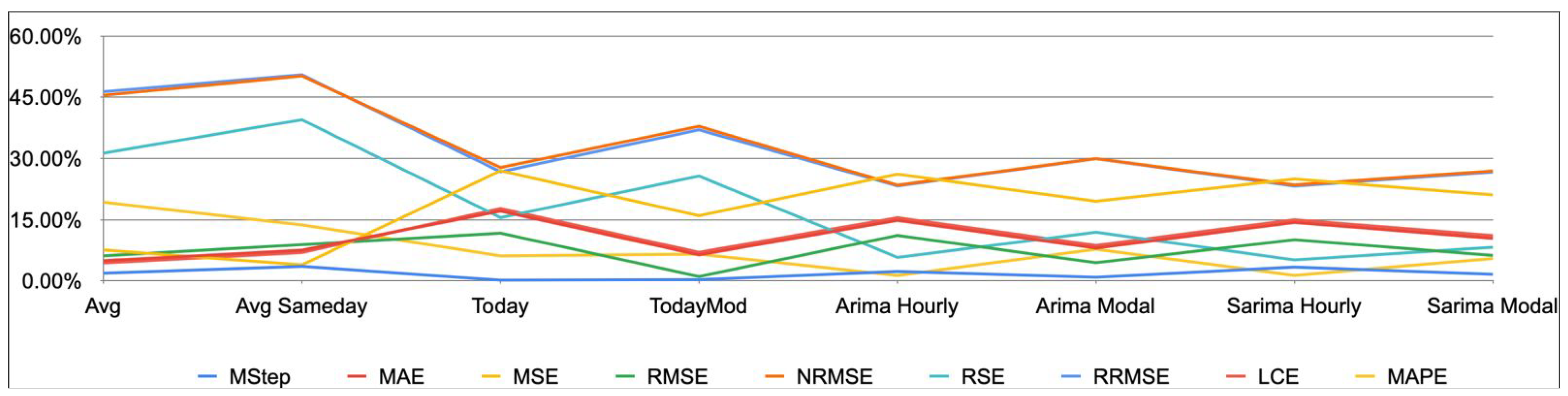
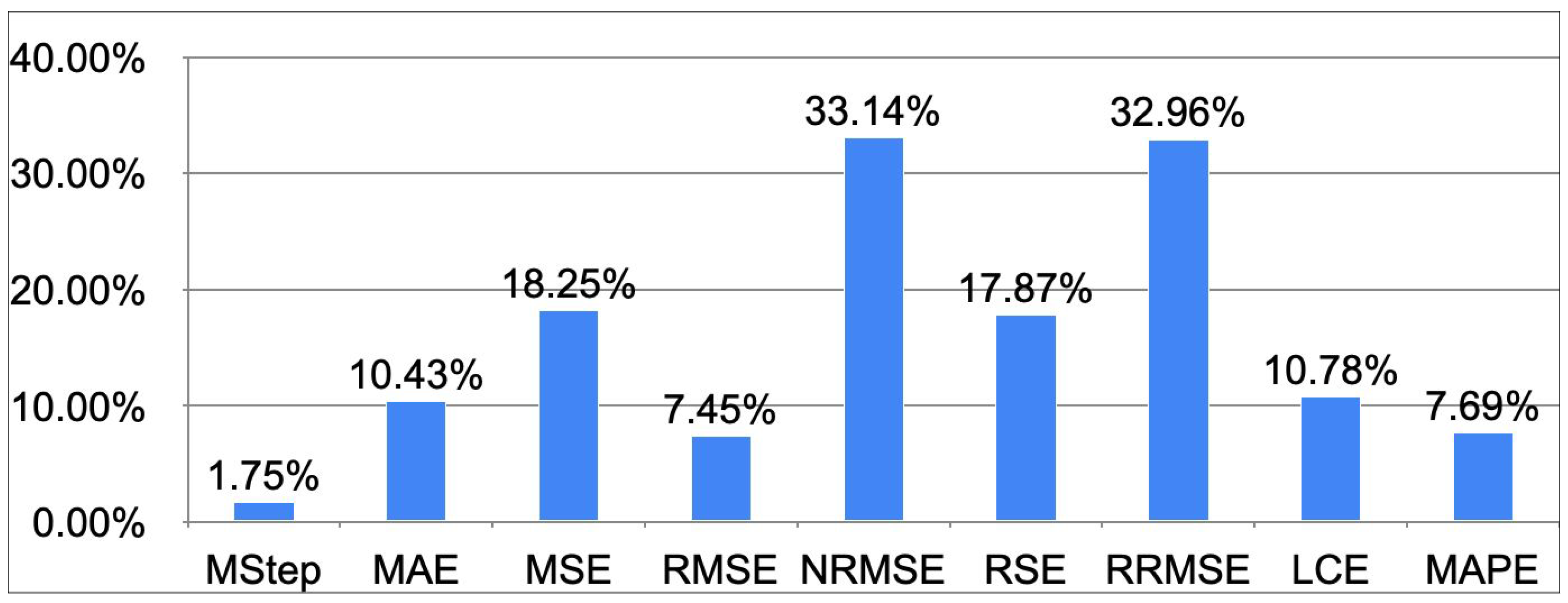
Disclaimer/Publisher’s Note: The statements, opinions and data contained in all publications are solely those of the individual author(s) and contributor(s) and not of MDPI and/or the editor(s). MDPI and/or the editor(s) disclaim responsibility for any injury to people or property resulting from any ideas, methods, instructions or products referred to in the content. |
© 2024 by the authors. Licensee MDPI, Basel, Switzerland. This article is an open access article distributed under the terms and conditions of the Creative Commons Attribution (CC BY) license (https://creativecommons.org/licenses/by/4.0/).