Article

Large Drawdowns and Long-Term Asset Management

by
Eric Jondeau
1,*,† and
Alexandre Pauli
2,†
1
Faculty of Business and Economics (HEC Lausanne), Swiss Finance Institute and CEPR, University of Lausanne, CH 1015 Lausanne, Switzerland
2
Ecole Polytechnique Fédérale de Lausanne, Route Cantonale, CH 1015 Lausanne, Switzerland
*
Author to whom correspondence should be addressed.
The authors contributed equally to this work.
J. Risk Financial Manag. 2024, 17(12), 552; https://doi.org/10.3390/jrfm17120552
Submission received: 22 October 2024 / Revised: 1 December 2024 / Accepted: 3 December 2024 / Published: 10 December 2024
(This article belongs to the Special Issue Featured Papers in Mathematics and Finance)

Abstract

:
Long-term investors are often hesitant to invest in assets or strategies prone to significant drawdowns, primarily due to the challenge of predicting these drawdowns. This study presents a multivariate Markov-switching model for small- and large-cap returns in the U.S. equity markets, demonstrating that three distinct regimes are necessary to capture the negative trends in expected returns during financial crises. Our findings indicate that this framework enhances the prediction of conditional drawdowns compared to standard alternative models of financial returns. Furthermore, out-of-sample analysis shows that investment strategies based on these predictions outperform those relying on models with one or two regimes.

1. Introduction

In recent decades, the recurrence of disasters has raised the issue of protecting investors’ portfolios from large market drawdowns.1 In the first quarter of 2020, the U.S. equity market experienced a 36 % decline—one of the five largest one-quarter drawdowns in the last century. Such substantial drawdowns are particularly significant for long-term asset managers, including insurers, pension funds, and sovereign wealth funds, as these losses can not only impact annual portfolio performance but may also threaten the survival of the fund. To mitigate these losses, some managers incorporate drawdown objectives into their portfolio optimization processes. However, modeling and predicting the temporal evolution of large drawdowns remains a considerable challenge, particularly as these events often unfold over extended periods (e.g., a quarter or a year), a time scale inconsistent with most conventional financial econometric models.
In this paper, we address both modeling and prediction challenges related to market drawdowns. We introduce a model for daily financial returns based on regime switches, which facilitates the prediction of significant market drawdowns. Our findings demonstrate that three distinct regimes are necessary to capture the long-term dynamics of U.S. stock market returns. Leveraging this model, we design an investment strategy aimed at minimizing the expected value of a large drawdown measure, possibly subject to an expected return target. We then evaluate this strategy out of sample over the last 30 years, providing evidence that investing according to this approach effectively allows investors to reduce their losses due to large market downturns, outperforming standard alternative models such as GARCH-type models.
Most of the literature exploring the prediction of large drawdowns relies on some form of historical simulation. For instance, Chekhlov et al. (2005) simulate scenarios based on historical data to predict next-period drawdowns. This approach is likely to work well in-sample but may not perform well when market conditions vary over time, possibly due to climate change. A key challenge in using parametric models to predict large drawdowns is that most models fail to capture large losses accumulating over relatively extended periods. In particular, standard GARCH models, even with nonnormal distributions, are not able to generate the negative trend that we observe during financial market crises. Consequently, reproducing large drawdowns similar to those observed in the 1999 dotcom crisis, the 2008 subprime crisis, or the 2020 COVID-19 pandemic becomes highly challenging with these models. In contrast, Markov-Switching (MS) models can generate large losses associated with a crisis because they allow for different drifts in market returns across regimes. Therefore, when a given return process enters a bear regime, it can accumulate negative values for relatively long periods of time. Papers describing these models for financial returns often overlook this long-term property because their main focus is on other features of the returns’ data generating process. In particular, Ang and Bekaert (2002), Ang and Chen (2002), and Guidolin and Timmermann (2004, 2007, 2008) used MS models to capture the nonnormality or the asymmetric correlation of returns. More recently, similar approaches were adopted to analyze the consequences in financial markets of disasters arising from climate change (Karydas and Xepapadeas 2019, and Barnett et al. 2020) or from the COVID-19 pandemic (Pagano et al. 2023). For shorter prediction horizons (e.g., 10 days), Peng et al. (2022) find that an MS model with two regimes is sufficient for measuring large drawdowns. For longer horizons, we provide evidence that three regimes are necessary to capture the occurrence of financial crises and subsequent drawdowns effectively.
The literature defines several concepts of large drawdowns. One widely accepted measure is the period maximum drawdown (MDD), which corresponds to the largest loss from peak to trough over a given period. Investment strategies based on MDD are analyzed by Grossman and Zhou (1993) in a continuous-time framework or by Reveiz and Leon (2008) in discrete time. Chekhlov et al. (2005) define the concept of conditional drawdown (CDD), which corresponds to an average of the largest drawdowns in a given period, with the average drawdown (ADD) and the MDD as limiting cases. More recently, Goldberg and Mahmoud (2016) define the conditional expected drawdown (CED), which corresponds to an average of the largest period MDD values over a long sample. These measures have interesting properties, as CDD and CED are convex measures of risk and as such can be reduced by portfolio diversification.
In this paper, we first evaluate the number of regimes necessary to predict large drawdowns. We perform this analysis using a long sample of daily returns for both small- and large-cap stocks, covering nearly 100 years, with the last 30 years used for out-of-sample evaluation.2 Given that small caps are more vulnerable to drawdowns than large caps, we assess whether a strategy focused on minimizing an expected large drawdown measure produces optimal weights that differ from those minimizing the portfolio variance. We estimate multivariate MS-GARCH models with one to four regimes and different distributions for the innovation process. We empirically demonstrate that three regimes are statistically necessary to fit the data while four regimes would not provide any additional information. In the three-regime model, one of the regimes has large negative expected returns, which allows us to generate large windfalls consistent with actual crises. In contrast, standard GARCH models fail to generate such extensive drawdowns.
We proceed by running an out-of-sample investment exercise. Using a rolling window, we estimate the various models and allocate the portfolio for the subsequent period. Although this experiment is time-consuming, it effectively mimics an investor’s real-time allocation process, penalizes overparameterized models, and helps mitigate the winner’s curse problem (Hansen 2009). We find that models with three regimes provide the best predictions of large drawdowns in this experiment. When allocating investor wealth by minimizing the predicted large drawdown measure for the upcoming period, the ex post drawdown of the portfolio is consistently lower with the three-regime model compared to the GARCH model or the two-regime model. Investors using the three-regime model tend to allocate long positions in large caps and short positions in small caps—an allocation that proves effective in mitigating large drawdowns.
Finally, we consider an investor aiming to maximize an expected return—large drawdown criterion, which also takes into account the model’s ability to predict expected returns. The out-of-sample results again demonstrate that one- and two-regime models are nearly always dominated by the three-regime models, particularly for extreme drawdowns.

2. Materials and Methods

2.1. Definitions and Measurement

The maximum drawdown is the most widely used concept of large drawdowns. It represents the maximum loss from peak to trough over a given time period. As MDD increases for longer time series, it is customary to measure MDD over a given fixed time period of one quarter or one year, for example. This section defines the notations and the various concepts of large drawdowns that we will analyze in the remainder of the paper.
Let p t = ( p t , 1 , , p t , H ) be a sample path associated with the stochastic process P with a continuous and strictly increasing distribution, where p t , h denotes the log-price on day h in period t (e.g., a given quarter or year).3 The drawdown within this period on day h corresponds to the return loss between the last peak and the current price:
D D t , h = max 1 j h p t , j p t , h .
We denote the drawdowns within the period as D D t = ( D D t , 1 , , D D t , H ) . The maximum drawdown is defined as the largest drawdown of the period:
M D D t = max 1 h H D D t , h .
Chekhlov et al. (2003, 2005) define the conditional drawdown (CDD) as the average of the largest drawdowns in a given period exceeding a quantile of the drawdown distribution, which mitigates the impact of outliers. For a probability θ , CDD is given by the average of the worst ( 1 θ ) × 100 % drawdowns. Formally, we define the drawdown threshold T h θ ( D D t ) as the θ -quantile of the drawdown distribution: T h θ ( D D t ) = inf { s | Pr ( D D t > s ) 1 θ } . CDD corresponds to the tail conditional expectation of the drawdown distribution, i.e., the average of the drawdowns above the threshold:
C D D θ , t = E t [ D D t | D D t > T h θ ( D D t ) ] ,
where the expectation is applicable over the sample path. When θ = 0 , C D D θ , t is equal to the average drawdown, A D D t = E t [ D D t ] . When θ 1 , C D D θ , t coincides with M D D t . For a given sample path p t , we have A D D t C D D θ , t M D D t .
Finally, Goldberg and Mahmoud (2015, 2016) introduce the concept of conditional expected drawdown (CED) as the average of the MDD values exceeding a quantile of the MDD distribution. For a probability θ ˜ , C E D θ ˜ corresponds to the average of the worst ( 1 θ ˜ ) × 100 % maximum drawdowns. Consequently, the threshold T h θ ˜ ( M D D ) is determined by the θ ˜ -quantile of the M D D distribution: T h θ ˜ ( M D D ) = inf { s | Pr ( M D D > s ) 1 θ ˜ } and the C E D θ ˜ is therefore given by:
C E D θ ˜ = E [ M D D | M D D > T h θ ˜ ( M D D ) ] ,
where the expectation is taken over the full sample. When θ ˜ = 0 , C E D θ ˜ is equal to the sample average period MDD, i.e., E [ M D D ] .
Similar to the well-known expected shortfall, which measures the tail conditional expectation of the return distribution, CDD and CED correspond to the tail conditional expectation of the drawdown distribution and the tail conditional expectation of the maximum drawdown distribution, respectively. Importantly, as shown by Chekhlov et al. (2005) and Goldberg and Mahmoud (2015), MDD, CDD, and CED satisfy the properties of deviation measures, i.e., nonnegativity, shift invariance, positive homogeneity, and convexity. Convexity of a measure of risk implies that this measure can be reduced by diversification and used in quantitative optimization. As a consequence, if an investor minimizes this measure, the minimum, if it exists, is a global minimum.
Our subsequent analysis will focus on the three large drawdown measures: CDD, MDD, and CED. An essential feature of these measures is that drawdowns can develop over different time frames.4 To cope with this feature, we consider three different horizons H, corresponding to one quarter, two quarters, and four quarters.

2.2. Empirical Measures of Large Drawdowns

We now briefly describe how to measure the ex post drawdown of an asset or a portfolio of assets. We match the horizon of the drawdown measures to a long-term investor’s horizon H. For instance, an asset manager rebalancing the portfolio every quarter wants to control for large drawdowns occurring throughout the quarter. Therefore, the full sample is divided into T nonoverlapping subsamples of length H, with the sequence of log-prices in subsample t given by p t = ( p t , 1 , , p t , H ) for t = 1 , , T . For each subsample, the vector of drawdowns is denoted by D D t = ( D D t , 1 , , D D t , H ) , with D D t , h = max 1 j h p t , j p t , h , as before.
We obtain the drawdown-based measures for each subsample as follows. The period ADD is simply given by the sample mean of the drawdowns, A D D t = 1 H h = 1 H D D t , h ; the period MDD is given by the maximum drawdown of the subsample, M D D t = max 1 h H D D t , h ; and the period CDD is calculated as the average of the drawdowns over the θ -quantile:
C D D θ , t = 1 ( 1 θ ) H h = 1 H D D t , h I ( D D t , h > T h θ , t ) ,
where I x = 1 if x is true and 0 otherwise, and T h θ , t = inf { s | 1 H h = 1 H I ( D D t , h > s ) 1 θ } .
Finally, CED is based on the distribution of the period MDD measures over the full sample: we collect the MDD values over all the subsamples M D D = ( M D D 1 , , M D D T ) and the sample CED corresponds to the average of the worst ( 1 θ ˜ ) × 100 % MDD values over the full sample:
C E D θ ˜ = 1 ( 1 θ ˜ ) T t = 1 T M D D t I ( M D D t > T h θ ˜ ) ,
where T h θ ˜ = inf { s | 1 T t = 1 T I ( M D D t > s ) 1 θ ˜ } .

2.3. Investor’s Problem

We now consider the investment strategy of a long-term investor with investment horizon H. At the end of period t, n risky assets are available. We denote by r i , t + 1 , h the log-return of asset i on day h of the period t + 1 . The vector of cumulated log-returns over h days is denoted by R t + 1 , h = { R i , t + 1 , h } i = 1 n , where R i , t + 1 , h = j = 1 h r i , t + 1 , j . Portfolio weights, determined at the end of period t, are denoted by α t = ( α 1 , t , , α n , t ) with i = 1 n α i , t = 1 . The (unknown) value of the portfolio at the end of period t + 1 is P t + 1 ( α t ) = α t exp ( R t + 1 , H ) in the absence of rebalancing during period t + 1 . The sequence of daily log-values of the portfolio in period t + 1 is given by: p t + 1 ( α t ) = ( p t + 1 , 1 ( α t ) , , p t + 1 , H ( α t ) ) , where p t + 1 , h ( α t ) = log P t + 1 , h ( α t ) and P t + 1 , h ( α t ) = α t exp ( R t + 1 , h ) .
For a given weight vector α t , we compute daily log-values in period t + 1 and obtain large drawdown measures as described in Section 2.2.5 The investment criterion consists of minimizing the expected value of one of the large drawdown measures for the next investment period (period CDD, MDD, or CED), which we denote generically as X D D t + 1 ( α t ) . The optimal weight is:
α t arg min { α t } E t [ X D D t + 1 ( α t ) ] .
We also consider a criterion based on the trade-off between the expected return and the risk of a large drawdown:
α t arg max { α t } E t [ R p , t + 1 ( α t ) ] λ 2 E t [ X D D t + 1 ( α t ) ] ,
where λ denotes the aversion for large drawdowns.
The minimization problem (5) corresponds to the case where the aversion for large drawdowns λ goes to infinity. Although the optimization problem (6) may be more attractive for an investor willing to combine risk and return, problem (5) allows us to investigate more specifically the ability of the various models to predict large drawdowns. In Section 3.4, we will focus our comments on the results based on problem (5) and briefly discuss problem (6).
To obtain predictions of portfolio large drawdown measures, i.e., E t [ X D D t + 1 ( α t ) ] , we proceed as follows: First, we assume a multivariate MS-GARCH model to describe the data generating process (DGP) for daily log-returns and endogenize the path dependence of the return process. Two-regime and three-regime models would capture the drawdown trend if switching probabilities are sufficiently low. Using this DGP, we simulate assets’ daily returns for the next investment period. Second, for a given portfolio weight vector, we obtain simulated paths of the portfolio return from which we deduce the large drawdown measures. This approach provides us with predictions of the large drawdown measures for the next investment period as a function of the weight vector, thereby enabling us to pinpoint the optimal weight that minimizes the objective function (Equation (5)). The details of our approach are the subject of the next section.

2.4. Methodology

2.4.1. Multivariate MS-GARCH Model

To capture the possible impact of a large drawdown on the performance of the long-term portfolio, we assume a multivariate MS-GARCH model for the return process. The vector of daily log-returns for the n assets is denoted by r ˜ d + 1 = ( r ˜ 1 , d + 1 , , r ˜ n , d + 1 ) . The temporal index d = 1 , , D , represents days and runs over the full sample.6
The model is written as follows:
r ˜ d + 1 = μ d + 1 ( S d + 1 ) + ε d + 1 ,
where μ d + 1 ( S d + 1 ) is the vector of expected returns, conditional on state S d + 1 , and ε d + 1 is the vector of unexpected returns. It is defined as:
ε d + 1 = Ω d + 1 ( S d + 1 ) 1 / 2 z d + 1 ,
where Ω d + 1 ( S d + 1 ) denotes the ( n × n ) covariance matrix of unexpected returns and z d + 1 is a sequence of iid innovations with distribution D ( 0 , I n ) with zero mean and identity covariance matrix.
States are defined by the Markov chain { S d + 1 } with K regimes and transition matrix P = p k k k , k = 1 , , K , where transition probabilities are p k k = Pr ( S d + 1 = k | S d = k ) , k , k { 1 , , K } .
Expected returns are constant within each state: μ d + 1 ( S d + 1 ) = μ ( k ) when S d + 1 = k .7 The covariance matrix Ω d + 1 ( S d + 1 ) is time- and state-dependent. In a given state k, it is driven by a multivariate GARCH process with state-dependent conditional correlation matrix, as in Pelletier (2006) or Haas and Liu (2018). The conditional variance of asset i in state k is defined as a standard univariate GARCH(1,1) process:8
σ i , d + 1 ( k ) 2 = ω i ( k ) + α i ( k ) ( r ˜ i , d μ i ( k ) ) 2 + β i ( k ) σ i , d ( k ) 2 ,
with different parameters for each state, as in Haas et al. (2004).
The ( n × n ) correlation matrix is constant in a given state: Γ ( k ) = ρ i j ( k ) i , j = 1 , , n , so that the covariance matrix Ω d + 1 ( S d + 1 ) = Ω d + 1 ( k ) in state k is:
Ω d + 1 ( k ) = ( D d + 1 ( k ) ) 1 / 2 Γ ( k ) ( D d + 1 ( k ) ) 1 / 2 ,
where D d + 1 ( k ) is the diagonal matrix with σ i , d + 1 ( k ) 2 i = 1 , , n on the diagonal.
We consider two types of multivariate distributions for innovations z d + 1 : A Gaussian distribution N ( 0 , I n ) and a standardized Student’s t distribution t ( 0 , I n , ν ) , where ν denotes the degree of freedom. The choice of the innovation distribution may matter for two reasons. First, for investors who care about higher moments, the investment criterion might involve metrics, such as large drawdowns, that depend on the properties of the innovation distribution. Second, in our model, large drawdowns can be captured in principle by a higher probability of being in a bear market or by negative expected returns in the bear regime. However, a lower degree of freedom of the Student’s t distribution can also affect the dynamics of regime shifts and possibly result in lower returns.9
To make inferences about the regimes, we calculate the probability of being in each regime. We denote by f ( r ˜ d + 1 | r ̲ ˜ d , θ ) the distribution of the daily log-return process conditional upon past log-returns, with r ̲ ˜ d = { r ˜ d , r ˜ d 1 , } and θ denoting the vector of unknown parameters. Parameters include expected returns ( μ ( k ) ), volatility parameters ( ω ( k ) , α ( k ) , β ( k ) ), correlations ( Γ ( k ) ), probabilities ( p k k ), and the degree of freedom ( ν ). Using Hamilton (1989)’s filter, we obtain the predicted probabilities π k , d + 1 = Pr [ S d + 1 = k | r ̲ ˜ d ] and the filtered probabilities ϕ k , d + 1 = Pr [ S d + 1 = k | r ̲ ˜ d + 1 ] as:
π d + 1 = P ϕ d + 1 and ϕ d + 1 = π d + 1 l d + 1 e ( π d + 1 l d + 1 ) ,
with l d + 1 = f ( r ˜ d + 1 | r ̲ ˜ d , S d + 1 = 1 ; θ ) f ( r ˜ d + 1 | r ̲ ˜ d , S d + 1 = K ; θ ) and e = ( 1 , , 1 ) .
The estimation of the model is based on standard likelihood maximization, where the log-likelihood is defined as: log L D ( θ ) = d = 1 D 1 f ( r ˜ d + 1 | r ̲ ˜ d , θ ) = d = 1 D 1 log k = 1 K π d + 1 l d + 1 . We impose stationarity conditions as described by Haas et al. (2004) and Abramson and Cohen (2007) in the univariate case and Haas and Liu (2018) in the multivariate case.10
While MS-GARCH models are valuable tools, they have certain limitations. To avoid overfitting, it is essential to carefully determine the number of regimes and ensure the model accurately captures the key patterns in the data. Estimating these models can be computationally demanding, especially because large datasets are needed for reliable results. This makes them less practical for systems with many variables or a high number of regimes. Additionally, the regimes must correspond to clear economic or financial conditions to make their interpretation meaningful. In our analysis, we address these challenges by using a simple model with only two processes, a long dataset, and by rigorously checking how well the model fits the data.

2.4.2. Minimizing the Expected Large Drawdown of a Portfolio

In some specifications of the multivariate MS model, analytical formulas for portfolio characteristics are available. For instance, Guidolin and Timmermann (2004, 2008) provide formulas for the high-order moments in a model with regime-dependent (but time-independent) means and variances. Other nonlinear characteristics, such as the VaR or the expected shortfall of the portfolio return distribution, cannot be computed analytically, even in this simple model (Guidolin and Timmermann 2004). Additionally, in models such as MS-GARCH, analytical expressions are usually not available because variances are path dependent. For this reason, we compute expected large drawdowns with Monte Carlo simulations.
For ease of exposition, we again assume a quarterly investment horizon, with H representing the number of days in a quarter. We solve the allocation problem (Equation (5)) at the end of quarter t through the following steps:
1.
We estimate the parameters of the MS-GARCH model using daily log-returns available in quarters 1 , , t . The last day of the estimation period is denoted by d = t × H . The next quarter, t + 1 , contains days d + 1 , , d + H .
2.
For a given estimated model, we simulate Q samples of length H of daily log-returns for the n assets: { r t + 1 , h ( q ) } h = 1 H , q = 1 , , Q . As the probability of being in state k at the end of period t is given by predicted probabilities { π d + 1 ( k ) } k = 1 K , we simulate a fraction π d + 1 ( k ) of the draws using Ω d + 1 ( k ) as an initial condition for the covariance matrix in period t + 1 . From the simulated daily log-returns, we compute cumulative log-returns in quarter t + 1 as: R t + 1 , h ( q ) = j = 1 h r t + 1 , j ( q ) for h = 1 , , H .
3.
For a portfolio weight vector α t , we obtain daily log-values of the portfolio: p t + 1 ( q ) ( α t ) = ( p t + 1 , 1 ( q ) ( α t ) , , p t + 1 , H ( q ) ( α t ) ) , where p t + 1 , h ( q ) ( α t ) = log ( α t exp ( R t + 1 , h ( q ) ) ) .
4.
We predict the risk measures with simulated daily log-prices of the portfolio. For each simulation q, we compute the drawdown measures using the definitions given in Section 2.2, yielding X D D t + 1 ( q ) ( α t ) . The predictions of the drawdown measures are then given by the average over the Q simulations: X D ^ D t + 1 ( α t ) = 1 Q q = 1 Q X D D t + 1 ( q ) ( α t ) , except for CED. To generate CED predictions, we rely on the MDD values obtained over all simulations M D D t + 1 ( α t ) = ( M D D t + 1 ( 1 ) ( α t ) , , M D D t + 1 ( Q ) ( α t ) ) and take the average of the worst ( 1 θ ˜ ) × 100 % MDD values as in Equation (4).
5.
We iterate points 3 and 4 over α t until the optimal portfolio weight vector α t is found for the investment problem (5). To solve investment problem (6), we also predict the expected return of the portfolio for the next quarter t + 1 as E t [ R p , t + 1 ( α t ) ] = 1 Q q = 1 Q exp p t + 1 , H ( q ) ( α t ) p t , H ( q ) ( α t ) 1 .
To obtain accurate estimates of the optimal weights, we simulate a large number of draws ( Q = 50,000 ).

3. Results

3.1. Data

Our empirical application is based on two size portfolios constructed using the Fama and French (1993) methodology. Small caps include the firms with the lowest market capitalization (bottom 30 % ), while large caps consist of the firms with the largest market capitalization (top 30 % ).11 The portfolios comprise all NYSE, AMEX, and NASDAQ stocks for which market equity data are available. The sample spans from July 1926 to December 2020, encompassing a total of 24,896 daily returns.12
Size portfolios offer several advantages for analyzing the construction of a portfolio in the context of large drawdowns. First, data on these portfolios is available over an extensive period (nearly 100 years). Second, size portfolios have been the focus of large attention for decades, making their properties relatively well understood, particularly in terms of their risk and return characteristics. Third, numerous studies have examined small-cap and large-cap stocks due to their distinct behaviors during crises and varying market conditions, such as bull and bear markets. Perez-Quiros and Timmermann (2000) provide evidence that small caps exhibit a high degree of asymmetry between recessionary and expansionary states. During recessions, small caps are more strongly impacted than large caps by deteriorating credit market conditions. Ang and Chen (2002) and Patton (2004) investigate the dependence between small and large caps, focusing on their asymmetric behavior during bull and bear markets. Huang et al. (2012) report that small firms are more exposed to extreme downside risks, and that the higher average returns of small caps actually compensate investors for the occurrence of larger drawdowns. The COVID-19 market crash illustrates this phenomenon: in the first quarter of 2020, small caps experienced a 45 % decline, whereas large caps decreased by only 33 % . From this perspective, we compare the optimal weights allocated to size portfolios based on the minimization of large drawdowns and the minimization of standard portfolio variance.
Table 1 reports statistics on small and large caps. Panel A corresponds to the full sample (1926–2020, 378 quarters), while Panel B focuses on the out-of-sample period that we used for the investment analysis (1990–2020, 124 quarters). The first part of the table displays descriptive statistics and standard risk measures. Small caps exhibit higher annual return and higher volatility on average. The Value-at-Risk (VaR) and expected shortfall (ES) measures demonstrate that small caps are more prone to large adverse shocks. The overall MDD is equal to 92 % for small caps and 86.5 % for large caps, corresponding in both cases to the stock market crash of 1929–1932.
The second part of the table reports the four sample measures of large drawdowns described in Section 2.2, for horizons of one quarter, two quarters, and four quarters. We compute CDD for a probability θ = 0.8 , i.e., we consider the average of the worst 20 % drawdowns in a given subsample (e.g., the worst 12 drawdowns in a given quarter) (see Chekhlov et al. 2005). We compute CED with a probability θ ˜ = 0.9 , which corresponds to the worst 10 % of MDD values in the sample (the worst 12 MDD values in the out-of-sample period) (see Goldberg and Mahmoud 2016). By examining the four period drawdown measures, we find that they also are all greater for small caps than large caps. On average, the one-quarter MDD on small caps is larger by approximately 2.3 % and the two-quarter MDD is larger by 4 % . ADD and CDD exhibit similar patterns. CED is also substantially higher for small caps than for large caps (by roughly 8 % over one quarter and 11 % over one year). This evidence suggests that, despite higher expected returns for small caps, investors may be reluctant to invest in small caps because they are more exposed to extreme downside risk, particularly over the long term, as suggested by Ang and Chen (2002) and Huang et al. (2012).
The table also reports relatively high first-order autocorrelation coefficients in ADD, CDD, and MDD measures in the full sample. The four-quarter MDD has AR(1) parameters equal to 48 % for small caps and 45 % for large caps. In the out-of-sample period (Panel B: 1990–2020), large drawdowns are much less persistent. The AR(1) parameter is usually low and close to 0 for small caps at all horizons, although it remains slightly higher for large caps. For the four-quarter MDD, the AR(1) parameters are equal to 11 % for small caps and 38 % for large caps.
Figure 1 presents the temporal evolution of the large drawdown measures. As expected, it reveals that, over the last century, four periods have been accompanied by large drawdowns: the Great Depression (1929–1933), the oil crisis (1973–1979), the subprime crisis (2008–2012), and the COVID-19 downturn (2020). The figure also displays the 10 % CED for each horizon over the full sample (horizontal lines on the right-hand side plots). With the four-quarter CED as a threshold, we identify only two exceptional drawdowns (the Great Depression and the subprime crisis episodes), whereas with the two-quarter CED we would also include the COVID-19 downturn as an exceptional event.

3.2. Full-Sample Model Estimation

In this section, we evaluate the ability of MS-GARCH models to predict large drawdowns over the full sample (1926–2020). This unique estimation helps interpret the parameter estimates and formally test the number of regimes and the choice of the innovation distribution. Table 2 and Table 3 report parameter estimates for the models with one, two, and three regimes, with normal and Student’s t innovations. Table 4 reports likelihood ratio (LR) test statistics, which we use to identify the model that best reproduces the data properties. We first consider the one-regime model, i.e., the standard multivariate GARCH model with constant conditional correlation. Parameter estimates of expected returns, volatility dynamics, and their correlation are fairly standard and similar for both innovation distributions. The degree of freedom of the Student’s t distribution is equal to 5.68 , which suggests that innovations have relatively heavy tails. The LR test rejects the null hypothesis that the distribution is normal.
The properties of the models with two regimes are very different depending on the distribution assumed. With normal innovations, the second regime has large negative expected returns for both assets. Two distinct regimes are clearly identified: the first regime pertains to normal conditions and the second regime corresponds to the bear state, possibly associated with market downturns. Our estimates are consistent with the high degree of asymmetry of small caps highlighted by Perez-Quiros and Timmermann (2000): In the bear market, expected returns are much lower for small caps than for large caps, probably reflecting tighter credit market conditions. The probability of remaining in the bear state is relatively low ( p 22 = 68.3 % ), with a stationary probability equal to 22 % .13
In contrast, with Student’s t innovations, the expected returns in Regime 2 are close to 0. The probability of remaining in the low regime is the same as the probability of remaining in the high regime ( p 11 = 96.3 % and p 22 = 96.7 % ), so that the stationary probability of being in Regime 2 is as high as π , 2 = 53 % . As a consequence, Regime 2 cannot be interpreted as a pure bear state. These results suggest that, in this model, the occurrence of large drawdowns is not captured by large negative expected returns but instead by the heavy-tailed nature of the Student’s t innovations.14
For the three-regime models, expected returns, volatility dynamics, and the correlation are similar for both innovation distributions. The results align with our expectations: Regime 1 captures the long periods during which the stocks are in a bull market (with high expected returns). Regime 2 corresponds to the slow growth or recovery regime, with intermediate expected returns. Regime 3 accounts for bear market conditions. As in the two-regime case, small caps have much higher expected returns than large caps in Regime 1 and much lower expected returns than large caps in Regime 3. Regime 3 also exhibits a higher correlation than Regime 1, reflecting the asymmetry in dependence found by Ang and Chen (2002).
The degree of freedom of the Student’s t distribution is equal to 7.8 , suggesting relatively thin tails compared to the two-regime model. Similar to the two-regime models, the Student’s t innovation partly captures the occurrence of large negative returns, as expected returns in Regime 3 are higher with Student’s t innovations. As a result, the stationary probability of being in Regime 3 is higher than in the model with normal innovations ( 30.4 % versus 19.5 % ).
A formal test of the number of regimes can be performed using the Likelihood-Ratio (LR) test but the usual asymptotic distribution of the test statistic does not hold. The reason is that, in the test of the null hypothesis that n 1 regimes are sufficient against the alternative of n regimes, parameters associated with the n-th regime are not identified under the null hypothesis and the regularity conditions justifying the χ 2 approximation to the LR test do not hold. Hansen (1992, 1996) proposed an LR test procedure that addresses this problem (see also Garcia 1998). Specifically, we adopt the strategy proposed by Ang and Bekaert (2002), which is based on Monte-Carlo simulations to obtain the finite-sample distribution of the LR test statistic.15 We implement this approach for all tests of the number of regimes from 1 to 3 (see Table 4). For 1 and 2 regimes, we reject the null hypothesis, with p-values all below 0.5 % , whatever the distribution of the innovation process. These tests indicate that the one-regime model should be rejected against the two-regime model and the two-regime model should be rejected against the three-regime model.
We also estimate four-regime models (with normal and Student’s t innovations) with our data and test whether 3 regimes are sufficient to match the data. Compared to three regimes, the gain in likelihood with four regimes is relatively large, but using the simulation-based LR distribution, we do not reject the null hypothesis of three regimes against four regimes, with a p-value equal to 20.2 % with the normal distribution and to 19 % with the Student’s t distribution.16
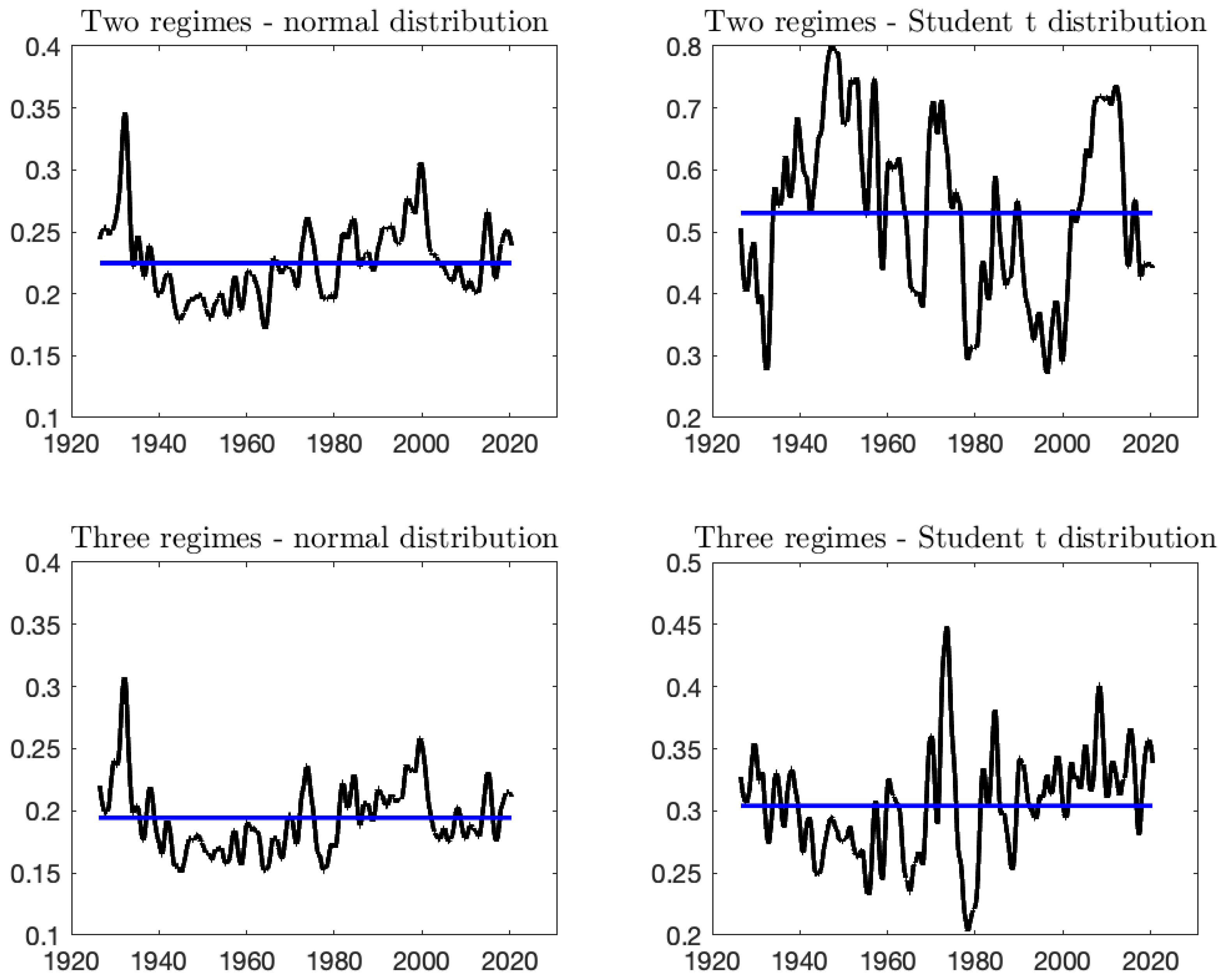
In Figure 2, we represent the filtered probability of being in the low regime for the two-regime and three-regime models. First, we note that the two-regime/Student’s t model produces a high filtered probability (on average above 50 % ), suggesting that this regime actually does not capture bear markets. Second, the filtered probabilities in the two-regime and three-regime models with normal innovations exhibit similar temporal evolution. Peaks occur at the same times with similar probabilities. However, these peaks do not always coincide with actual market downturns. The first peak occurs in June 1932, after the Wall Street crash of October 1929. The second peak corresponds to the oil crash in mid-1973. The third peak in May 1984 could not be associated with any market downturn. The fourth peak, which occurred in October 1999, corresponds to the dotcom crash. The last peak in September 2014 again does not correspond to any large market decline. Consequently, models with normally distributed innovations do not accurately capture observed market downturns.
In the three-regime model with Student’s t innovations, most peaks in the filtered probability actually correspond to market events associated with a long-lasting bear market. We can identify three main episodes: The first one corresponds to the bear market at the beginning of the period (with peaks in the second half of 1929 and at the end of 1937, associated with the Wall Street crash and the economic recession, respectively). The second episode corresponds to the inflationary bear market of the seventies (with peaks at the end of 1969 and mid-1973).17 The third episode is associated with the market crashes at the turn of the new century (Russian crisis in 1998, dotcom crash in 2001 and financial crisis in 2008). In the more recent period, the filtered probability also increased in mid-2015 (associated with the stock market sell-off following the ending of quantitative easing by the Federal Reserve) and at the beginning of 2020 (associated with the COVID-19 market crash).18
The analysis of filtered probabilities clearly suggests that the three-regime/Student’s t model provides a better description of the market downturns observed in the sample period than the other competing models.
Another related interesting feature of MS models is that they can generate asymmetry in the distribution of returns even if the volatility dynamics and the innovation distribution are symmetric. The reason for this property is the possible shift from one regime to another, which generates relatively large (positive or negative) events. To assess whether the various models are able to generate the asymmetry that we observe in the data (see Table 1), we simulate long trajectories of the small caps and large caps daily returns and compute the skewness of the simulated series. As reported in Table 5, the one-regime models do not generate any asymmetry because this property is absent from the model. Two-regime models are able to produce some asymmetry but it is clearly insufficient to match the data. For instance, in the normal distribution case, the skewness measures of the small caps and large caps returns are equal to 0.19 and 0.16 , respectively. This is well above the sample skewness that we obtained over the full sample ( 0.39 for small caps and 0.48 for large caps, respectively). In contrast, three-regime models produce skewness measures that are in the ball park of the sample measures. In the normal model, the skewness estimates are equal to 0.8 and 0.5 for small caps and large caps, respectively. In the Student’s t model, the values are equal to 0.5 and 0.3 . Again, this analysis suggests that three regimes are necessary to match the extreme behavior of actual returns.
The table also reports predictions of the large drawdown measures for the three horizons. Again, one-regime models and the two-regime/Student’s t model fail at capturing the magnitude of large drawdown measures obtained with the data, by substantially underestimating drawdowns. The two-regime/normal model is able to capture the magnitude of drawdowns on average but fail at generating the asymmetry observed between small caps and large caps. The drawdowns are usually similar for both size portfolios. In contrast, three-regime models are able to generate this asymmetry, although it is often not as large as with the observed data.

3.3. Rolling-Window Model Estimation and Adequacy Tests

To implement the out-of-sample allocation strategy, we use a rolling window to estimate the parameters of the MS-GARCH models over subsample periods. For each model, the first set of parameters is estimated over the sample of daily returns from January 1927 to December 1989, while the last window covers the sample from January 1958 to December 2020. These parameter estimates will be used to simulate paths of daily log-returns of length H and predict next-period drawdown measures.
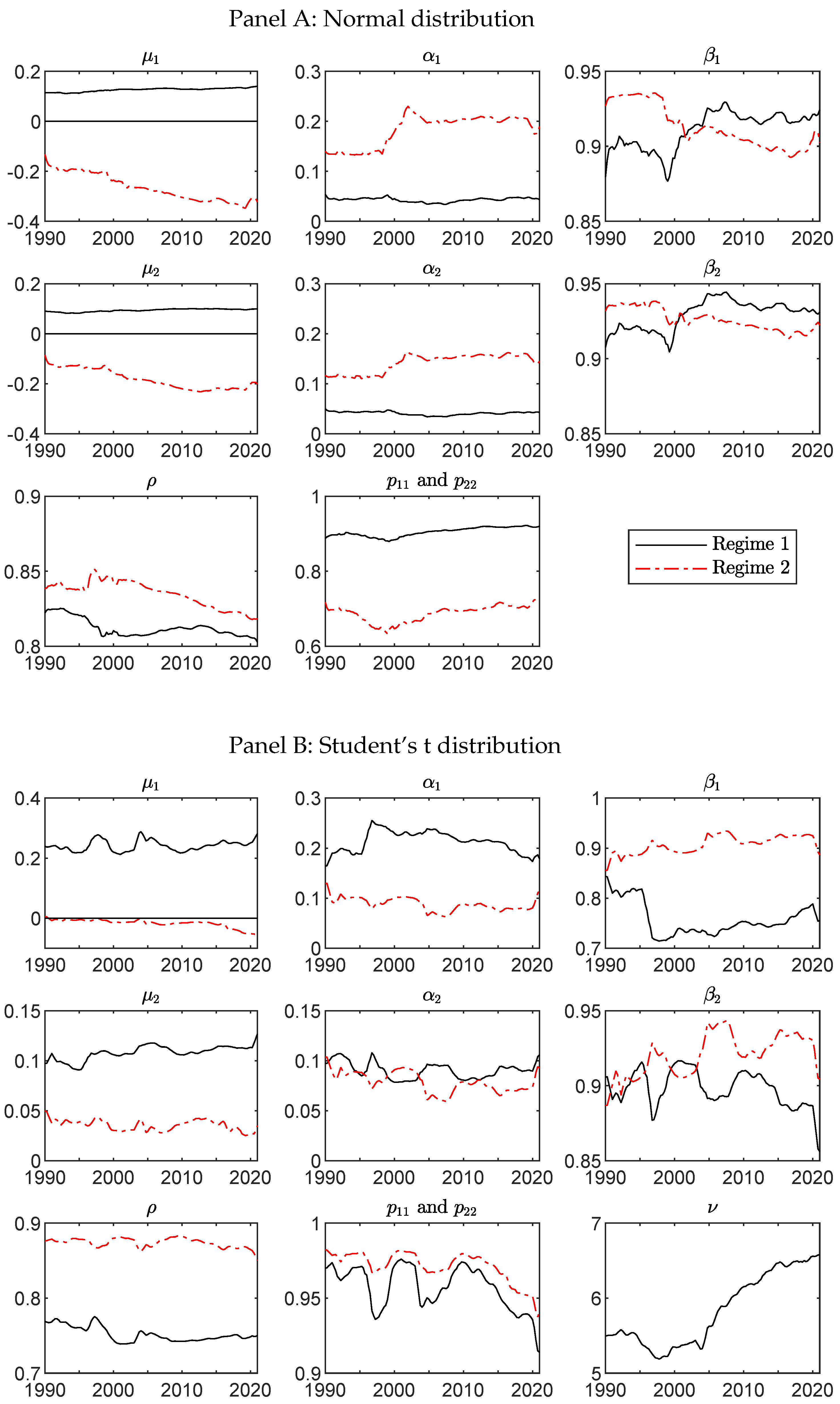
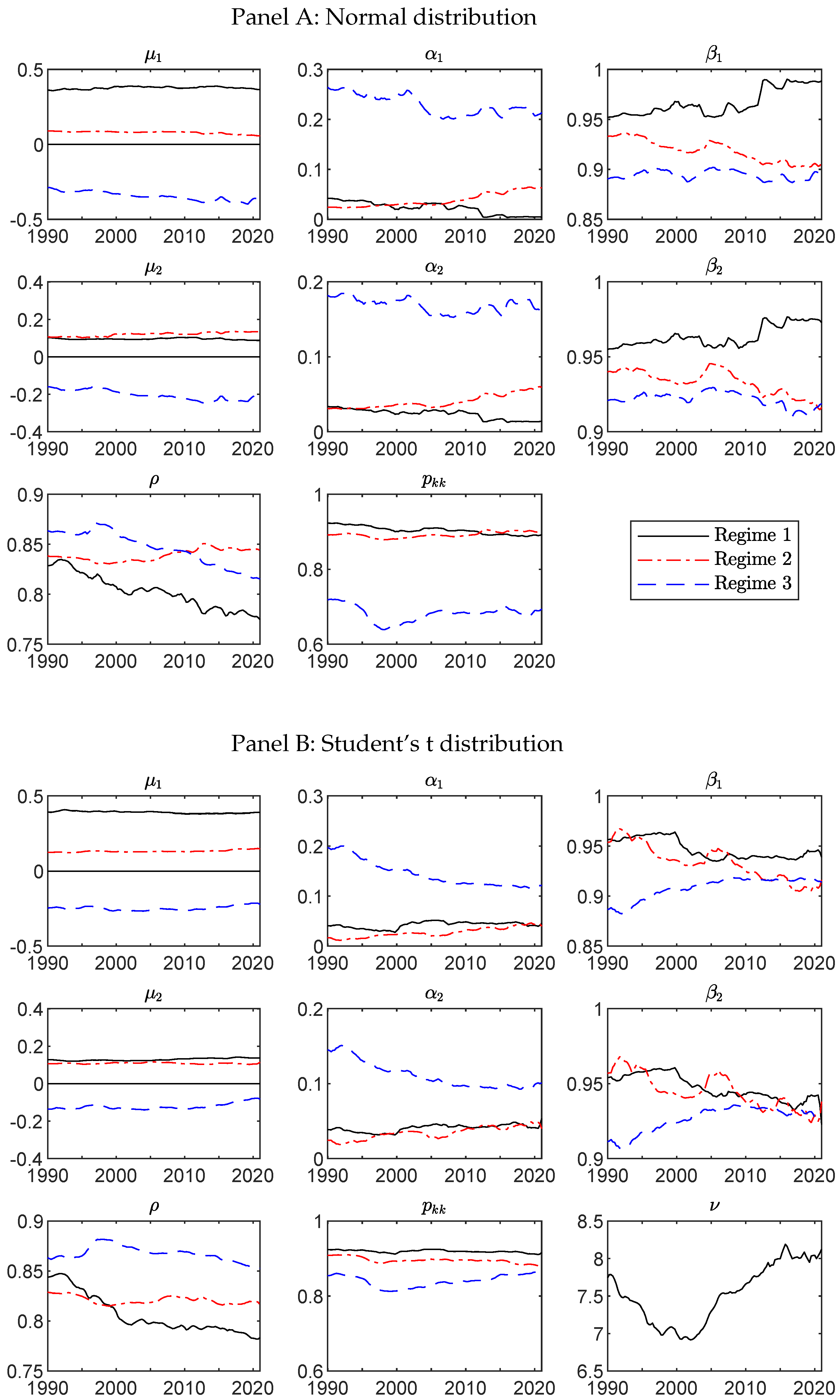
The temporal evolution of parameter estimates for the competing models is displayed in Appendix A. Comparison with the full sample estimates in Table 2 and Table 3 reveals a remarkable match between the two sets of estimates on average. The figures demonstrate that parameter estimates are usually rather stable over time, although a few parameters exhibit trends. In particular, the correlation between small and large caps tends to decrease in Regimes 1 and 3 in the three-regime model. The degree of freedom of the Student’s t distribution tends to increase in the two-regime and three-regime models.
We assess the adequacy of out-of-sample estimation of our models with respect to returns for small and large caps by backtesting predicted C D D ^ θ , t and M D D ^ t obtained through simulations.19 To perform these tests, we adopt the approach proposed by Acerbi and Szekely (2014) for testing expected shortfall estimates. We adjust their testing framework for the unconditional coverage of the CDD measure.
The methodology and the main results are reported in Appendix B. In a nutshell, our adequacy tests reveal that one- and two-regime models inaccurately predict drawdown measures for both small and large caps. Specifically, the one-regime and two-regime/Student’s t models underestimate drawdown measures, while the two-regime/normal and three-regime/normal models overestimate realized CDD and MDD for large caps. The one-regime and two-regime/Student’s t models systematically underestimate drawdown measures for both small and large caps. The only model that perform relatively well for both small and large caps is the three-regime/Student’s t model, with the expected number of exceedances and average drawdown above the threshold being close to the numbers observed in the data.

3.4. Out-of-Sample Analysis

We now consider investors who allocate their wealth in real time period by period, with an investment horizon from one quarter to one year between 1990 and 2020. The out-of-sample strategy is implemented as follows. We use the rolling-window estimation of the models to predict next-period drawdown measures. With these predictions, we determine the optimal portfolio weight that minimizes the expected drawdown measures. Next, we roll the window by one period (H days) and proceed in the same way until we reach the last subsample (ending in September 2020). This out-of-sample analysis corresponds to 124 nonoverlapping quarterly allocations and 31 nonoverlapping annual allocations.
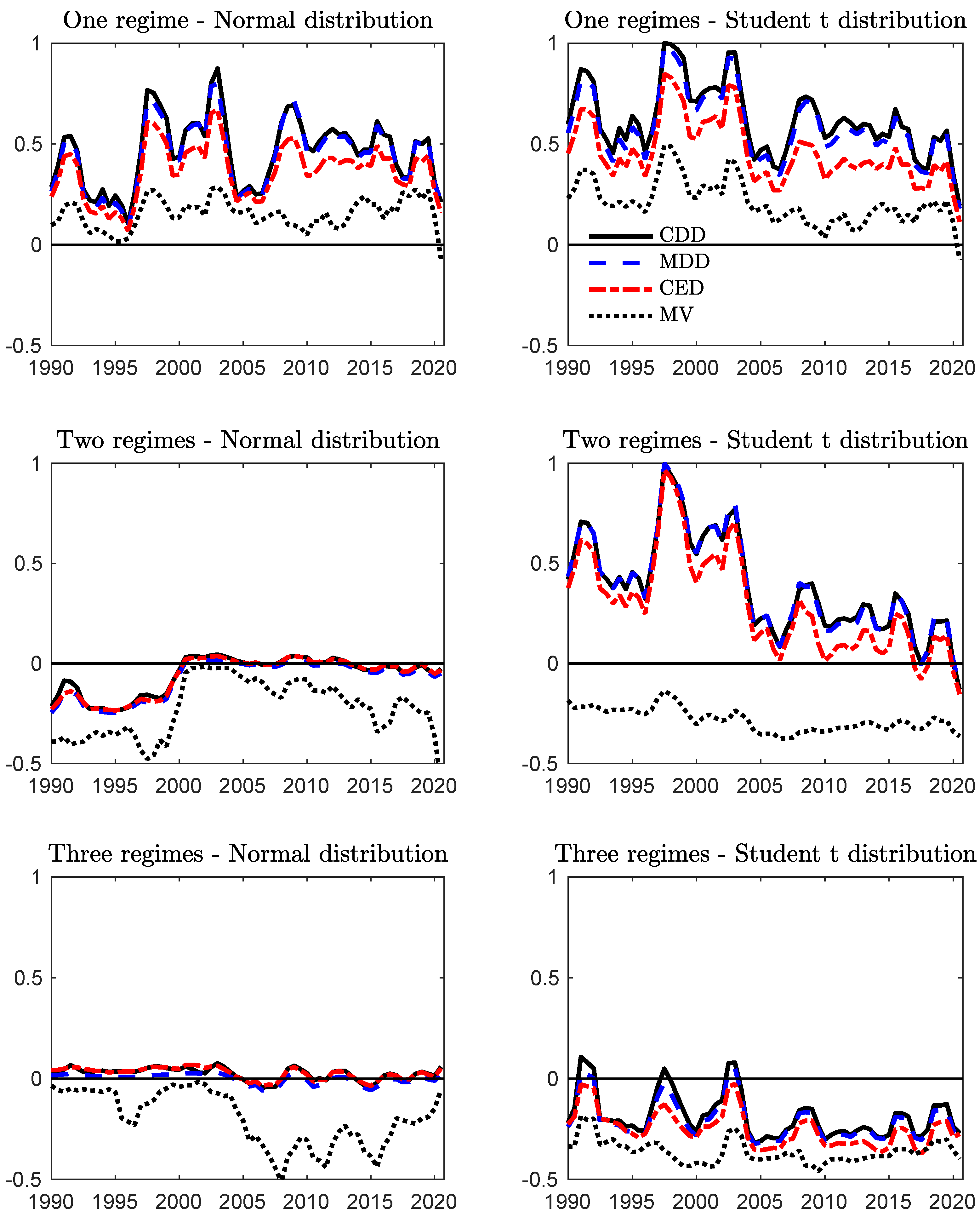
Figure 3 displays the evolution of the optimal small-cap weights obtained by minimizing large drawdown measures based on the various models for a two-quarter horizon. As illustrated, the evolution of optimal weights exhibits notable differences across the approaches used for prediction. For the one-regime models and the two-regime/Student’s t model, the optimal small-cap weights are all positive, regardless of the targeted large drawdown measure. This finding implies that a diversified portfolio, with weights close to 50 % , could provide effective diversification against large drawdowns. This result indicates that these models do not effectively generate the large drawdowns observed in the small-cap portfolio. Conversely, the two-regime/normal and three-regime/normal models display similar patterns, with optimal small-cap weights close to 0. This suggests that the innovation process plays a critical role in generating sufficiently large drawdowns for small caps, potentially resulting in negative weights.
The three-regime model/Student’s t model displays optimal weights that are usually negative. This finding can be explained by the ability of the three-regime/Student’s t model to generate large and negative expected returns in a relatively long-lasting Regime 3, which allows large drawdowns in small caps to develop and therefore to identify that holding small caps implies higher tail risk. As a consequence, this model produces large negative weights for most allocation criteria and investment horizons.20
In general, the optimal weights are ordered in the same way for the various investment criteria: the weight of small caps is higher for CDD, then for MDD, and finally for CED. We compare these weights with those resulting from the minimization of the portfolio variance. Minimum variance (MV) portfolio weights are obtained using the same simulation approach. Results indicate that, for all investment horizons, the optimal weight of the MV portfolio is always negative, in the range [ 40 % ; 20 % ] for the two-regime and three-regime models. Figure 3 also demonstrates that the weight of small caps is systematically lower for the MV criterion than for criteria based on large drawdowns.21
These patterns suggest that investors targeting large drawdowns tend to be even more cautious in their allocation than MV investors, as they are reluctant to take substantial short positions in small caps.
Table 6 reports results for the out-of-sample allocation when the investor minimizes the expected value of large drawdowns. We compare the performance of the allocation based on the various parametric models. The standard (one-regime) multivariate GARCH models (with normal and Student’s t distributions) and the two-regime/Student’s t models fail at capturing that the risk of large drawdowns is higher for small caps. Therefore, these models generate a large weight on average for small caps, for all investment horizons. As small caps experienced larger drawdowns than large caps in our sample, strategies based on these models tend to underperform and suffer from much higher ex post drawdowns on average. For instance, for the two-quarter CDD, strategies based on these models have average small caps weights equal to 0.46 , 0.63 , and 0.39 , respectively. Their ex post two-quarter CDD values are equal to 8.47 % , 9.16 % , and 8.30 % on average. In contrast, the two-regime/normal model and the three-regime models (with normal and Student’s t distributions) tend to have negative small cap weights on average, with substantially lower ex post two-quarter CDD values, equal to 7.23 % , 7.26 % , and 7.15 % , respectively.
It is worth emphasizing that, in all cases, the strategies based on the standard multivariate GARCH models result in much larger drawdown measures than strategies based on three-regime models. The gap is economically substantial for the three measures CDD, MDD, and CED. The ex post four-quarter CDD of the one-regime/normal model is 2.1 points higher that the same measure of the three-regime/Student’s t model. The difference is equal to 2.3 points for the four-quarter MDD and 1.7 points for the four-quarter CED. The gaps are less severe for the two-regime/normal model but they remain large for long horizons. They are equal to 2.4 points for the four-quarter CDD, 0.6 point for the four-quarter MDD, 0.4 point for the four-quarter CED.
Overall, the three-regime/normal model performs well for the one-quarter horizon, while the three-regime/Student’s t model performs the best for the two- and four-quarter horizons. In all cases, the best models generate an optimal weight that is negative or close to 0.
We also consider an investor maximizing the expected return—large drawdown criterion (Equation (6)), which also accounts for the ability of the models to predict expected returns. Results are reported in Table 7 with a degree of aversion for large drawdowns equal to λ = 5 . Optimal weights for small caps are usually higher, reflecting the higher expected return of small caps. For the one-regime models and the two-regime/Student’s t model, small caps weights are even often larger than one, indicating the large caps are shorted in these allocations. Turning to the two-regime/normal model and three-regime models, we find that weights are also higher than in the case of the minimization of large drawdowns but to a lesser extent. For the MDD and CED targets, small caps weights are negative for a short horizon but close to 50 % for two-quarter and four-quarter horizons. These results indicate that investors also targeting the expected return would invest more in small caps because of their higher return on average.
Regarding the performance of the strategies, we obtain essentially the same conclusions as before. One-regime models are always dominated by models with at least two regimes. In addition, three-regime models usually outperform other models, in particular for extreme drawdowns (MDD and CED). To illustrate the gain of using a three-regime model to predict large drawdowns, we compute the opportunity cost of using a one-regime or two-regime model, using the relation:
E t [ R p , t + 1 ( α t ( s u b ) ) ξ ( s u b ) ] λ 2 E t [ X D D t + 1 ( α t ( s u b ) ) ] = E t [ R p , t + 1 ( α t ( o p t ) ) ] λ 2 E t [ X D D t + 1 ( α t ( o p t ) ) ] ,
where α t ( s u b ) and α t ( o p t ) denote the vector of weights obtained using the suboptimal model and the optimal model, respectively. The opportunity cost ξ ( s u b ) is defined as the fraction of the expected return that an investor using the suboptimal strategy is ready to pay to get access to the optimal strategy.
The estimates of the opportunity cost are also reported in the table. For the one-quarter investment horizon, the best strategy is the one based on the three-regime/normal model. In this case, an investor using the two-regime/normal model would be ready to pay 1 % if the objective function is targeting the MDD and 1.8 % if the objective function is targeting the CED. For the two-quarter investment horizon, the best strategy is the one based on the three-regime/Student’s t model. In this case, an investor using the two-regime/normal model would be ready to pay 3.4 % if the objective function is targeting the MDD and up to 9 % if the objective function is targeting the CED. As these estimates illustrate, the gain of using a three-regime model is economically substantial for investors targeting large drawdown measures.
This out-of-sample analysis demonstrates that three regimes are necessary in the multivariate MS-GARCH model to produce large and negative weights for small caps. Student’s t innovations also help generate a longer-lasting bear state and therefore to produce more drawdowns for small caps. Importantly, as the allocation exercise is performed in a fully out-of-sample fashion, we account for the risk of over-parameterization of the three-regime models.

4. Conclusions

This paper addresses the modeling and prediction of large drawdowns in financial markets. Given that the standard GARCH model struggles to capture prolonged market declines, we explore multivariate MS-GARCH models, which can generate regimes characterized by both positive and negative market trends. Provided that the probability of remaining in a bear regime is sufficiently high, these models are capable of reproducing significant drawdown properties. Specifically, our findings show that in three-regime models, one regime is marked by substantial negative expected returns (representing a bear market) and the capacity to generate large windfalls.
In the out-of-sample investment analysis, as changes in the distribution of drawdowns are updated, three-regime models prove to be superior tools for predicting expected drawdowns by imposing restrictions that align well with the observed data. These models consistently outperform other parametric models featuring one regime (such as standard multivariate GARCH models) or two regimes.
To assess the predictive power of MS-GARCH models for large drawdowns, we intentionally keep our model specification straightforward within a well-established framework, ensuring robust results. Notably, we do not attempt to identify factors influencing the dynamics of state probabilities, which may be affected by variables related to government or monetary policies, geopolitical issues, or climate change, among others.22 Exploring these factors represents an important avenue for future research.

Author Contributions

Conceptualization, E.J. and A.P.; methodology, E.J. and A.P.; validation, E.J. and A.P.; writing—original draft preparation, E.J. and A.P.; writing—review and editing, E.J. and A.P.; supervision, E.J. All authors have read and agreed to the published version of the manuscript.

Funding

This research received no external funding.

Data Availability Statement

All data used in this paper are from Kenneth French’s website: https://mba.tuck.dartmouth.edu/pages/faculty/ken.french/data_library.html, accessed on 2 December 2024.

Conflicts of Interest

The authors declare no conflicts of interest.

Appendix A. Evolution of Model Parameters
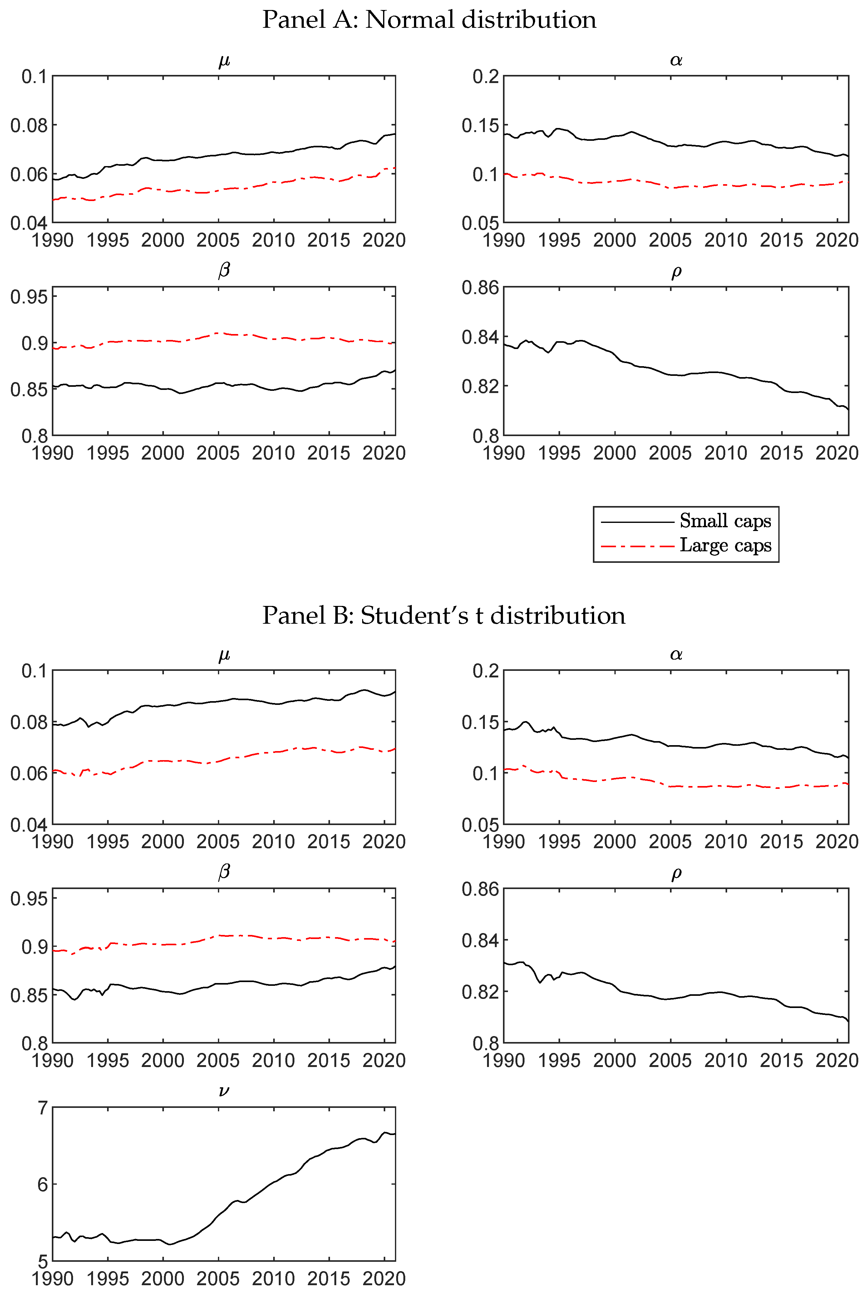
Figure A1. Model Parameters: One-regime Models.
Jrfm 17 00552 g0a1
Figure A2. Model Parameters: Two-regime Models.
Jrfm 17 00552 g0a2
Figure A3. Model Parameters: Three-regime Models.
Jrfm 17 00552 g0a3

Appendix B. Adequacy Tests

Our predictions of the large drawdown risk measures, generically defined as X D D ^ t , are obtained by simulations from the models. Therefore, by backtesting X D D ^ t , we assess whether the model underlying a particular prediction is adequate. To backtest our predicted risk measures, we rely on the second test by Acerbi and Szekely (2014). Note that Acerbi and Szekely (2017) propose a more robust approach for backtesting a risk measure that depends on another statistic, such as ES or CDD, which depend on a threshold. The proposed ridge backtest accounts for the sensitivity of the statistic to the threshold estimation by penalizing errors in estimation. However, this test is only relevant for validating a model from a prudential perspective, that is, testing that the model does not underestimate the risk measure. Therefore, this procedure is not suitable for testing the CDD. As we want to assess if a model tends to overestimate or underestimate the CDD, we do not pursue with this test. The backtest for M D D ^ t does not suffer from the sensitivity to the threshold.

Appendix B.1. Logic of the Adequacy Test

The logic of the test is the following: For a given risk measure, we define a Z statistic that is equal to zero under the null hypothesis that the model correctly predicts this risk measure:
E H 0 [ Z X D D ( X D D ^ , D D ) ] = 0 ,
where D D is a random variable representing drawdowns. Then, from the sequence of risk measure predictions and drawdowns realizations, we compute the realized Z statistic over the out-of-sample period:
z X D D = 1 T t = 1 T Z X D D ( X D D ^ t , D D t ) ,
where D D t is the vector of observed drawdowns defined in Section 2.2.
Finally, we test the adequacy of a given model by comparing the realized Z statistic obtained from this model to the distribution of the Z statistics under the null hypothesis. This distribution is obtained by computing Z statistics from simulations of the model over the out-of-sample period.23

Appendix B.2. Adequacy Test Statistics

For ease of exposition, we assume that the distribution is continuous and strictly increasing, as in Section 2.1.
For CDD, we build the Z statistic from the fact that C D D θ , t = E t [ D D t I ( D D t > T h θ , t ) ] , where T h θ , t = inf { s | 1 H h = 1 H I ( D D t , h > s ) 1 θ } , with E t [ T h θ , t ] = ( 1 θ ) H . The test statistic is defined as (see Equation (3)):
z C D D = 1 T t = 1 T h = 1 H D D t , h I ( D D t , h > T h ^ θ , t ) ( 1 θ ) H C D D ^ θ , t 1 ,
where C D D ^ θ , t and T h ^ θ , t are predictions of C D D θ , t and T h θ , t based on simulations of the model estimated using data until quarter t 1 , and T corresponds to the number of quarters in the out-of-sample period.
The hypotheses for this test are as follows:
H 0 : C D D θ , t C D D ^ θ , t = 0 for all t H 1 : | C D D θ , t C D D ^ θ , t | > 0 for some t .
Under the null hypothesis, we have E H 0 [ Z C D D ( C D D ^ , D D ) ] = 0 . Under the alternative hypothesis, if the model underestimates the CDD, we have E H 1 [ Z C D D ( C D D ^ , D D ) ] > 0 , and if the model overestimates the CDD, we have E H 1 [ Z C D D ( C D D ^ , D D ) ] < 0 . The test actually jointly evaluates the frequency and the magnitude of the tail events because the test statistics do not impose that h = 1 H I ( D D t > T h ^ θ , t ) = ( 1 θ ) H , i.e., the frequency is correct. Therefore, the test statistic will be close to 0 if both the predicted threshold is close to the realized threshold and the predicted CDD is close to the realized CDD.
For MDD, we simply define the Z statistic as:
z M D D = 1 T t = 1 T M D D t M D D ^ t 1 ,
where M D D ^ t = 1 Q q = 1 Q M D D t ( q ) is the prediction of M D D t based on model’s simulations.
The hypotheses of this test are:
H 0 : M D D t M D D ^ t = 0 for all t H 1 : | M D D t M D D ^ t | > 0 for some t .
It follows that E H 0 [ Z M D D ( M D D ^ , D D ) ] = 0 under the null hypothesis that the model correctly describes the realized MDD. When the model underestimates (overestimates) the risk measure, the Z statistic takes a positive (negative) value, i.e., E H 1 [ Z M D D ( M D D ^ , D D ) ] 0 .

Appendix B.3. Adequacy Test Significance

To find the test significance, we generate Z statistics under the null hypothesis by simulating the model for which we test the adequacy. Then, by comparing the realized Z statistic to the simulated Z statistic under H 0 , we evaluate the p-value, i.e., the probability to obtain the realized Z statistic from the model underlying the null hypothesis. We proceed as follows:
  • Using the model under H 0 , we simulate Q samples of log-returns for all quarters of the backtesting period: { r t ( q ) } h = 1 H , t = 1 , , T and q = 1 , , Q . The simulations are generated as in Section 2.4.2.
  • We calculate the vectors of drawdowns for each simulation, D D t ( q ) , t = 1 , , T . Then, we compute Z statistic for each simulation, z X D D ( q ) = z X D D ( X D D ^ , D D ( q ) ) , q = 1 , , Q . They represent the distribution of the Z statistic under the null hypothesis.
  • We compute the realized Z statistic on the drawdowns z X D D ( q ) = z X D D ( X D D ^ , D D ) .
  • We estimate the significance by comparing the realized Z statistic to the distribution of the simulated Z statistics and compute the p-value of the bilateral test as: p-val = 1 1 Q q = 1 Q ( | z X D D ( q ) | < | z X D D | ) .

Appendix B.4. Adequacy Test Results

Results of the adequacy tests are reported in Table A1. The statistics are based on 50,000 simulations of the estimated models. The table indicates that most models fail to capture the time-series properties of large drawdown statistics. The one-regime models and the two-regime/Student’s t model systematically underestimate the drawdown measures for both small and large caps. For CDD, the expected number of exceedances is equal to 1562 (i.e., 20 % of the total number of daily observations in the out-of-sample period). The one-quarter number of exceedances for the two-regimes/Student’s t model is equal to 2666 and 1961 for small caps and large caps, respectively, meaning that the estimated threshold is too low. As a consequence, the estimated CDD is too small, resulting in high values of the test statistic Z C D D ( D D ) . For all three models and all three investment horizons, p-values for the CDD and MDD tests are below 1.5 % . The reason for this failure is that these models do not allow for a negative trend in expected returns, and therefore, they cannot reproduce long-lasting market declines.
The two-regime/normal model and the three-regime/normal model provide a good description of the CDD and MDD of small caps, with p-values above 5 % for all three horizons. However, both models fail at correctly predicting the drawdown measures of large caps. They systematically overestimate the realized CDD and MDD for large caps. For large caps, the one-quarter number of exceedances is close to 1000 for both models, while the expected number is equal to 1562.
The only model that performs relatively well for small caps and large caps is the three-regime/Student’s t model. For CDD, it produces a number of exceedances and an average drawdown above the threshold, which is close to the numbers observed in the data. For the one-quarter horizon, the numbers of exceedances equal 1800 and 1412 for the small caps and large caps, respectively, while the expected number is 1562. The p-value of the test statistic is equal to 2.8 % for small caps and to 66.7 % for large caps, suggesting that the 20 % threshold on drawdowns is slightly too small for small firms. Similarly, this model performs relatively well for the two-quarter horizon, with a number of exceedances and an average drawdown above the threshold, which is in line with the data.
Table A1. Adequacy Tests for Out-of-sample Predictions (1990–2020).
1-Regime1-Regime2-Regime2-Regime3-Regime3-Regime
NormalStudent tNormalStudent tNormalStudent t
SmallLargeSmallLargeSmallLargeSmallLargeSmallLargeSmallLarge
Panel A: 20 % CDD
1 quarter
Nb exc.259717812961196414901015266619611512108218001412
Stat.1.6930.6532.3100.8760.052−0.3071.6930.8290.039−0.2820.3080.055
p-val.(0.000)(0.000)(0.000)(0.000)(0.666)(0.007)(0.000)(0.000)(0.762)(0.018)(0.028)(0.667)
2 quarters
Nb exc.2930193834432221116869729672173127878414421124
Stat.2.1650.6873.1340.987−0.134−0.5452.1670.891−0.063−0.4840.037-0.266
p-val.(0.000)(0.000)(0.000)(0.000)(0.210)(0.000)(0.000)(0.000)(0.367)(0.001)(0.396)(0.033)
4 quarters
Nb exc.316317283863211710375103243203712446131193683
Stat.2.0610.4493.2850.794−0.328−0.6492.2370.662−0.186−0.567−0.238−0.545
p-val.(0.000)(0.015)(0.000)(0.001)(0.066)(0.000)(0.000)(0.003)(0.218)(0.002)(0.138)(0.002)
Panel B: MDD
1 quarter
Stat.0.6220.2660.8850.377−0.047−0.2020.7390.363−0.033−0.1920.078−0.009
p-val.(0.000)(0.000)(0.000)(0.000)(0.327)(0.000)(0.000)(0.000)(0.538)(0.000)(0.176)(0.852)
2 quarters
Stat.0.8020.2841.1680.423−0.057−0.2850.9190.383−0.010−0.237−0.033−0.188
p-val.(0.000)(0.000)(0.000)(0.000)(0.305)(0.000)(0.000)(0.000)(0.862)(0.000)(0.595)(0.002)
4 quarters
Stat.0.8730.2901.2860.435−0.045−0.2991.0170.3630.021−0.232-0.059−0.269
p-val.(0.000)(0.000)(0.000)(0.000)(0.503)(0.000)(0.000)(0.000)(0.773)(0.001)(0.404)(0.000)
Note: This table reports the test statistics and the p-value for 20 % CDD and MDD. For CDD, the table also reports the number of exceedances, with an expected number equal to 1562. We consider three investment horizons: one quarter, two quarters, and four quarters. These results are based on the predictions of the models between 1990 and 2020.

Notes

1
Disasters may include severe macroeconomic and financial crises, pandemics, wars, or extreme weather and climate conditions.
2
We use a large sample to estimate model’s parameters accurately and perform the out-of-sample analysis over a long period of time. Such a long sample would not be necessary in practice to estimate MS models and to predict subsequent large drawdowns.
3
For simplicity, we assume here a fixed number of days H per period. In the empirical analysis, we will use the actual number of days per period.
4
A drawdown may span over a short period (as for the COVID-19 crisis, with a 36 % drawdown in 24 days) or over a window of more than a year (as for the subprime crisis, with a 60 % drawdown in 355 days).
5
We note that the knowledge of the cumulated log-return at the end of the period is not sufficient to infer the large drawdown measures, as peaks and troughs are likely to occur on random days within the period.
6
The model is estimated over a long sample of daily returns, ( r ˜ 1 , , r ˜ D ) , where D is the number of days in the full sample. In contrast, large drawdown measures are computed over relatively short subsamples (e.g., one quarter or one year) with H days, which we have denoted by r t = ( r t , 1 , , r t , H ) , t = 1 , , T in Section 2. Since we use nonoverlapping subsamples, both notations define the same sample: ( r ˜ 1 , , r ˜ D ) = ( r 1 , , r T ) , where D = H × T .
7
Assuming an autoregressive process would have a very limited effect for a long-term investment objective because the autocorrelation of daily returns is low. The first-order autocorrelation of the market return is equal to 0.05 over the 1926–2020 period and equal to 0.06 over the 1990–2020 period.
8
In this expression, we follow the suggestion of Klaassen (2002) and Haas et al. (2004) and define shocks with respect to a given state using the conditional mean μ i ( k ) instead of the unconditional mean μ i adopted by Gray (1996).
9
In Section 3.2, we use simulations to demonstrate that a three-regime model with a (symmetric) Student’s t innovations can generate some asymmetry in large drawdowns, as observed in the data.
10
We note that stationarity conditions apply to the complete distribution and not regime by regime. As a consequence, usual stationarity conditions in a GARCH model might not be satisfied for some regimes. In particular, global stationarity can be obtained even when α i ( k ) + β i ( k ) 1 for some asset i and regime k.
11
We have also analyzed the cases of firms in the bottom and top 20 % and 10 % market capitalization, with limited impact on the main results. The data are available on the website of Kenneth French at (https://mba.tuck.dartmouth.edu/pages/faculty/ken.french/data_library.html, accessed on 2 December 2024). Other long-sample portfolios, such as value versus growth or losers versus winners portfolios, are also available.
12
Our sample ends in December 2020, slightly after the end of the COVID-19 market crash. Therefore, the impact of this episode on the financial performance of our investment strategies is reflected in the out-of-sample analysis discussed in Section 3.4.
13
Stationary (or steady-state) probabilities are defined as: π = P π . In the two-regime case, this relation boils down to π , 2 = Pr [ S t = 2 ] = ( 1 p 11 ) / ( 1 p 11 p 22 ) .
14
This conclusion appears very robust and not driven by the choice of starting values. We experimented with several sets of starting parameter values and obtained the same parameter estimates for both models. A similar phenomenon—where the probability of remaining in the bear state is lower with normal innovations than with Student’s t innovations—was reported by Haas and Paolella (2012) and Haas and Liu (2018).
15
The finite-sample distribution of the LR statistic is obtained by simulating many samples of returns, using the estimated parameters of the ( n 1 ) -regime model and estimating, for each simulated samples, the ( n 1 ) -regime model and the n-regime model, from which we compute the LR test statistics. The finite-sample distribution of the LR test statistic is computed from the empirical distribution of the LR statistics based on the simulated samples.
16
Guidolin and Timmermann (2007) estimate MS model for U.S. small caps, large caps, and long-term bonds. In a specification with within-regime constant expected returns, volatilities, and correlations, they find that four regimes are necessary to match the data. In their model, the intermediate regime is further decomposed into a slow growth regime and a recovery regime.
17
The largest spike in the filtered probability of being in the bear state is associated with the 1973 oil crisis. The drawdown actually started in January 1973, accelerated in October with the surge in oil price and lasted until December 1974, with a drawdown of 48% over this period. A major feature of this 1973–1974 drawdown is its duration. From peak to through, the downturn lasted for almost 2 years, while the subprime crisis was associated with a 60% drawdown in slightly more than 1 year.
18
As in the models with normal innovations, one of the peaks in the filtered probability, in mid-1984, could not be associated with any particular stock market event.
19
Although we developed a similar test for CED, the number of observations was insufficient for robust conclusions.
20
We note that, even with our preferred model, i.e., the three-regime model with Student’s t distribution, the relationship between the probability of being in the bear regime (Figure 2) and the optimal small-cap weight (Figure 3) is far from perfect. The reason is that the probability of being in the bear regime predicts the state for the next day, whereas the portfolio is allocated for a long horizon (from 1 quarter to 1 year) and the regime is likely to change over this period.
21
This result of a lower small-cap weights for the MV criterion does not seem to be driven by a theoretical relation between the variance and large drawdown measures but more likely by the properties of our data.
22
For instance, Gray (1996) allows state probabilities to depend on lagged interest rates in an MS-GARCH model for short-term interest rates.
23
Note that Acerbi and Szekely (2014) assume a one-sided test in line with Basel VaR tests, which are designed to detect excesses of VaR exceptions. In our case, we assume a two-sided test, as we test whether a given model correctly predicts large drawdown measures.

References

  1. Abramson, Ari, and Israel Cohen. 2007. On the stationarity of Markov-switching GARCH processes. Econometric Theory 23: 485–500. [Google Scholar] [CrossRef]
  2. Acerbi, Carlo, and Balazs Szekely. 2014. Backtesting Expected Shortfall. Risk 27: 76–81. [Google Scholar]
  3. Acerbi, Carlo, and Balazs Szekely. 2017. General Properties of Backtestable Statistics. Working Paper. New York: MSCI Inc. Available online: https://ssrn.com/abstract=2905109 (accessed on 25 February 2023).
  4. Ang, Andrew, and Geert Bekaert. 2002. International asset allocation with regime shifts. Review of Financial Studies 15: 1137–87. [Google Scholar] [CrossRef]
  5. Ang, Andrew, and Joseph Chen. 2002. Asymmetric correlations of equity portfolios. Journal of Financial Economics 63: 443–94. [Google Scholar] [CrossRef]
  6. Barnett, Michael, William Brock, and Lars Peter Hansen. 2020. Pricing uncertainty induced by climate change. Review of Financial Studies 33: 1024–66. [Google Scholar] [CrossRef]
  7. Chekhlov, Alexei, Stanislav Uryasev, and Michael Zabaranki. 2003. Portfolio optimization with drawdown constraints. In Asset and Liability Management Tools. Edited by Berndt Scherer. London: Risk Books, pp. 263–78. [Google Scholar]
  8. Chekhlov, Alexei, Stanislav Uryasev, and Michael Zabaranki. 2005. Drawdown measure in portfolio optimization. International Journal of Theoretical and Applied Finance 8: 13–58. [Google Scholar] [CrossRef]
  9. Fama, Eugene F., and Kenneth R. French. 1993. Common risk factors in the returns on stocks and bonds. Journal of Financial Economics 33: 3–56. [Google Scholar] [CrossRef]
  10. Garcia, Rene. 1998. Asymptotic null distribution of the likelihood ratio test in Markov switching models. International Economic Review 39: 763–88. [Google Scholar] [CrossRef]
  11. Goldberg, Lisa R., and Ola Mahmoud. 2015. On a Convex Measure of Drawdown Risk. Working Paper. Berkeley: Center for Risk Management Research. Available online: http://arxiv.org/abs/1404.7493 (accessed on 25 March 2021).
  12. Goldberg, Lisa R., and Ola Mahmoud. 2016. Drawdown: From practice to theory and back again. Mathematics and Financial Economics 11: 275–97. [Google Scholar] [CrossRef]
  13. Gray, Stephen F. 1996. Modeling the conditional distribution of interest rates as a regime-switching process. Journal of Financial Economics 42: 27–62. [Google Scholar] [CrossRef]
  14. Grossman, Sanford, and Zhongquan Zhou. 1993. Optimal investment strategies for controlling draw-downs. Mathematical Finance 3: 241–276. [Google Scholar] [CrossRef]
  15. Guidolin, Massimo, and Allan Timmermann. 2004. Value at Risk and Expected Shortfall Under Regime Switching. Working Paper. San Diego: University of California. Available online: https://ssrn.com/abstract=557091 (accessed on 1 May 2021).
  16. Guidolin, Massimo, and Allan Timmermann. 2007. Asset allocation under multivariate regime switching. Journal of Economic Dynamics and Control 31: 3503–44. [Google Scholar] [CrossRef]
  17. Guidolin, Massimo, and Allan Timmermann. 2008. International asset allocation under regime switching, skew, and kurtosis preferences. Review of Financial Studies 21: 889–935. [Google Scholar] [CrossRef]
  18. Haas, Markus, and Ji-Chun Liu. 2018. A multivariate regime-switching GARCH model with an application to global stock market and real estate equity returns. Studies in Nonlinear Dynamics and Econometrics 22: 1–27. [Google Scholar] [CrossRef]
  19. Haas, Markus, Stefan Mittnik, and Marc S. Paolella. 2004. A new approach to Markov-switching GARCH models. Journal of Financial Econometrics 2: 493–530. [Google Scholar] [CrossRef]
  20. Haas, Markus, and Marc S. Paolella. 2012. Mixture and regime-switching GARCH models. In Handbook of Volatility Models and Their Applications. Edited by Luc Bauwens, Christian M. Hafner and Sebastien Laurent. Hoboken: John Wiley & Sons, pp. 71–102. [Google Scholar]
  21. Hamilton, James D. 1989. A new approach to the economic analysis of nonstationary time series and the business cycle. Econometrica 57: 357–84. [Google Scholar] [CrossRef]
  22. Hansen, Bruce E. 1992. The likelihood ratio test under non-standard conditions: Testing the Markov switching model of GNP. Journal of Applied Econometrics 7: S61–S82. [Google Scholar] [CrossRef]
  23. Hansen, Bruce E. 1996. Inference when a nuisance parameter is not identified under the null hypothesis. Econometrica 64: 413–30. [Google Scholar] [CrossRef]
  24. Hansen, Peter Reinhard. 2009. In-Sample Fit and Out-of-Sample Fit: Their Joint Distribution and Its Implications for Model Selection. Working Paper. Stanford: Department of Economics, Stanford University. [Google Scholar]
  25. Huang, Wei, Qianqiu Liu, S. Ghon Rhee, and Feng Wu. 2012. Extreme downside risk and expected stock returns. Journal of Banking and Finance 36: 1492–502. [Google Scholar] [CrossRef]
  26. Karydas, Christos, and Anastasios Xepapadeas. 2019. Climate Change Financial Risks: Pricing and Portfolio Allocation. Economics Working Paper Series, No. 19/327, 327. Zurich: Center of Economic Research (CER-ETH). [Google Scholar] [CrossRef]
  27. Klaassen, Franc. 2002. Improving GARCH volatility forecasts with regime-switching GARCH. Empirical Economics 27: 363–94. [Google Scholar] [CrossRef]
  28. Pagano, Marco, Christian Wagner, and Josef Zechner. 2023. Disaster resilience and asset prices. Journal of Financial Economics 150: 103712. [Google Scholar] [CrossRef]
  29. Patton, Andrew. 2004. On the out-of-sample importance of skewness and asymmetric dependence for asset allocation. Journal of Financial Econometrics 2: 130–68. [Google Scholar] [CrossRef]
  30. Pelletier, Denis. 2006. Regime switching for dynamic correlations. Journal of Econometrics 131: 445–73. [Google Scholar] [CrossRef]
  31. Peng, Cheng, Young Shin Kim, and Stefan Mittnik. 2022. Portfolio optimization on multivariate regime switching GARCH model with normal tempered stable innovation. Journal of Risk and Financial Management 15: 230. [Google Scholar] [CrossRef]
  32. Perez-Quiros, Gabriel, and Allan Timmermann. 2000. Firm size and cyclical variations in stock returns. Journal of Finance 55: 1229–62. [Google Scholar] [CrossRef]
  33. Reveiz, Alejandro, and Carlos Leon. 2008. Efficient portfolio optimization in the wealth creation and maximum drawdown space. In Interest Rate Models, Asset Allocation and Quantitative Techniques for Central Banks and Sovereign Wealth Funds. Edited by Arjan B. Berkelaar, Joachim Coche and Ken Nyholm. London: Palgrave Macmillan, pp. 134–157. [Google Scholar]
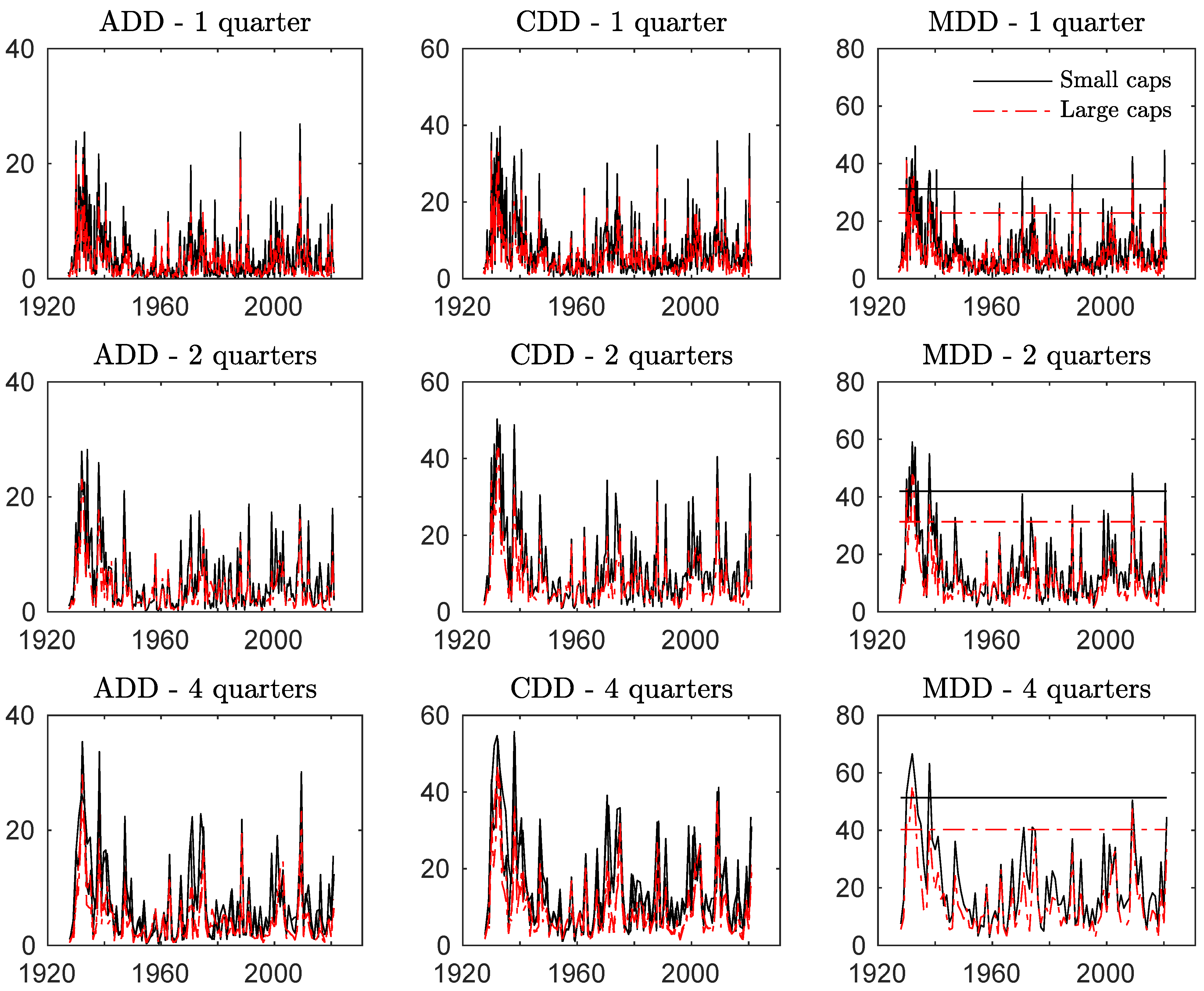
Figure 1. Evolution of ADD, CDD, and MDD over non-overlapping subsamples. The figure displays the evolution in percentage of ADD, 20 % CDD, and MDD over various non-overlapping subsamples (from one to four quarters) between 1926 and 2020. The straight line on right plots corresponds to 10 % CED. The black lines correspond to the small caps, the red dashed lines to the large caps. CED is computed with 376, 188, and 94 observations for the one-quarter, two-quarter, and four-quarter horizons, respectively.
Jrfm 17 00552 g001
Figure 2. Filtered Probability of Being in the Bear State. The figure displays the filtered probability ϕ d + 1 of being in the low expected return regime (bear state), for the two-regime and three-regime models. The horizontal blue line corresponds to the stationary probability of being in the bear state π b , = Pr [ S d + 1 = k b ] , where k b denotes the bear state.
Jrfm 17 00552 g002
Figure 3. Out-of-Sample Optimal Weights—Two-quarter Horizon (1990–2020). The figure displays the temporal evolution of the optimal weight of small caps for the 20 % CDD, MDD, 10 % CED, and MV portfolios over the two-quarter horizon, when predictions are based on the one-regime, two-regime, and three-regime models.
Jrfm 17 00552 g003
Table 1. Summary statistics on daily returns and period drawdowns for small caps and large caps.
Panel A: 1926–2020Panel B: 1990–2020
Small CapsLarge CapsSmall CapsLarge Caps
Daily returnsStat. Stat. Stat. Stat.
Annualized Mean10.63 8.99 10.38 9.88
Annualized Std dev.19.50 17.15 20.36 18.06
Skewness−0.39 −0.48 −0.81 −0.40
Kurtosis23.61 21.83 13.40 14.03
Maximum20.42 14.15 8.02 11.16
Minimum−16.75 −20.94 −14.26 −12.57
VaR ( 0.1 % )8.53 6.86 9.01 7.56
VaR ( 1 % )3.70 3.11 3.72 3.26
VaR ( 5 % )1.82 1.56 1.97 1.74
ES ( 0.1 % )10.76 9.16 11.24 9.32
ES ( 1 % )5.55 4.64 5.50 4.76
ES ( 5 % )3.09 2.62 3.17 2.77
Overall MDD92.02 86.54 67.13 58.29
Period drawdownsStat.AR(1)Stat.AR(1)Stat.AR(1)Stat.AR(1)
ADD - 1Q3.840.152.780.203.650.122.470.25
ADD - 2Q5.620.293.850.425.190.003.300.35
ADD - 4Q7.520.464.820.426.16−0.103.830.35
20 % CDD - 1Q7.750.255.760.287.280.125.270.23
20 % CDD - 2Q11.800.418.200.4610.810.057.140.30
20 % CDD - 4Q16.650.4510.960.4313.990.018.870.33
MDD - 1Q9.870.337.550.349.340.177.100.26
MDD - 2Q15.050.4410.930.4713.990.069.930.28
MDD - 4Q21.520.4815.230.4518.670.1113.080.38
10 % CED - 1Q31.22 22.84 25.97 20.60
10 % CED - 2Q41.97 31.35 35.40 25.41
10 % CED - 4Q51.37 40.25 38.36 31.19
Note: This table reports statistics (in percentage) on daily returns for small caps and large caps. Panel A covers the period from 1926 to 2020. Panel B covers the period from 1990 to 2020. VaR( α ) and ES( α ) denote the Value-at-Risk and Expected Shortfall computed for probability α . “XDD - nQ” means that the XDD measure is computed over n quarters. “ 20 % CDD” means that the CDD measure is computed for probability θ = 20 % . “ 10 % CED” means that the CED measure is computed for probability θ ˜ = 10 % .
Table 2. Parameter estimates for one-regime and two-regime models.
One regime—Normal distributionOne regime—Student’s t distribution
Small capsLarge capsSmall capsLarge caps
param.std err.param.std err.param.std err.param.std err.
Expected returns
μ ( × 100 )0.0679(0.006)0.0588(0.005)0.0865(0.004)0.0687(0.004)
Volatility dynamics
ω ( × 100 )1.4840(0.201)0.9667(0.122)0.9902(0.093)0.7532(0.071)
α 0.1298(0.008)0.0984(0.006)0.1220(0.007)0.0970(0.004)
β 0.8654(0.008)0.8962(0.006)0.8764(0.006)0.9010(0.004)
Correlation
ρ 0.8291(0.003) 0.8212(0.002)
Degree of freedom
ν 5.6810(0.154)
Log-lik.−48,291.3 −46,183.1
BIC96.6736 92.4674
Two regimes—Normal distributionTwo regimes—Student’s t distribution
Small capsLarge capsSmall capsLarge caps
param.std err.param.std err.param.std err.param.std err.
Expected returns
μ ( 1 ) ( × 100 )0.1265(0.007)0.0965(0.006)0.2093(0.035)0.1155(0.012)
μ ( 2 ) ( × 100 )−0.2706(0.043)−0.1771(0.030)−0.0276(0.016)0.0207(0.010)
Volatility dynamics
ω ( 1 ) ( × 100 )0.2974(0.052)0.3132(0.049)1.2510(0.293)0.8278(0.140)
α ( 1 ) 0.0418(0.005)0.0417(0.004)0.2055(0.021)0.1309(0.017)
β ( 1 ) 0.9209(0.008)0.9289(0.006)0.7968(0.020)0.8663(0.019)
ω ( 2 ) ( × 100 )0.1550(0.380)0.5501(0.279)0.1576(0.169)0.2482(0.195)
α ( 2 ) 0.1868(0.024)0.1463(0.019)0.0411(0.023)0.0422(0.021)
β ( 2 ) 0.9173(0.011)0.9291(0.008)0.9563(0.023)0.9565(0.022)
Correlation
ρ ( 1 ) 0.8179(0.004) 0.7450(0.014)
ρ ( 2 ) 0.8334(0.006) 0.8884(0.010)
Transition probabilities
p 11 0.9081(0.009) 0.9626(0.024)
p 22 0.6828(0.027) 0.9669(0.019)
Degree of freedom
ν 6.2260(0.252)
Log-lik.−45,974.7 −45,420.1
BIC92.1478 91.0507
Note: See Table 3 for details.
Table 3. Parameter estimates for three-regime model.
Three Regimes—Normal DistributionThree Regimes—Student’s t Distribution
Small CapsLarge CapsSmall CapsLarge Caps
param.std err.param.std err.param.std err.param.std err.
Expected returns
μ ( 1 ) ( × 100 )0.3304(0.022)0.1174(0.011)0.3194(0.017)0.1251(0.011)
μ ( 2 ) ( × 100 )0.0754(0.008)0.0966(0.007)0.1193(0.008)0.1133(0.008)
μ ( 3 ) ( × 100 )−0.3451(0.024)−0.1897(0.024)−0.2316(0.017)−0.1049(0.020)
Volatility dynamics
ω ( 1 ) ( × 100 )0.0001(0.191)0.1797(0.108)0.5529(0.205)0.4921(0.141)
α ( 1 ) 0.0403(0.019)0.0325(0.009)0.1303(0.022)0.0927(0.013)
β ( 1 ) 0.9480(0.022)0.9534(0.012)0.8585(0.022)0.8945(0.013)
ω ( 2 ) ( × 100 )0.2705(0.046)0.3461(0.060)0.0201(0.200)0.0858(0.040)
α ( 2 ) 0.0401(0.005)0.0439(0.004)0.0122(0.003)0.0177(0.003)
β ( 2 ) 0.9180(0.008)0.9233(0.006)0.9739(0.006)0.9691(0.006)
ω ( 3 ) ( × 100 )0.0001(0.640)0.8492(0.405)0.1357(0.310)0.6340(0.358)
α ( 3 ) 0.2262(0.033)0.1655(0.022)0.1328(0.031)0.1050(0.022)
β ( 3 ) 0.9005(0.018)0.9246(0.011)0.9145(0.022)0.9306(0.017)
Correlation
ρ ( 1 ) 0.7814(0.025) 0.7300(0.016)
ρ ( 2 ) 0.8487(0.006) 0.8465(0.009)
ρ ( 3 ) 0.8462(0.008) 0.8764(0.007)
Transition matrix
P 1 , : 0.92060.01690.0453 0.94020.01700.0266
(0.015)(0.003)(0.018) (0.009)(0.004)(0.007)
P 2 , : 0.03500.89540.2663 0.01650.91160.1139
(0.016)(0.008)(0.026) (0.007)(0.011)(0.013)
P 3 , : 0.04450.08770.6884 0.04330.07150.8595
(0.008)(0.006)(0.021) (0.008)(0.009)(0.014)
Degree of freedom
ν 7.7750(0.399)
Log-lik.−45,282.0 −44,852.6
BIC90.9244 90.0753
Note: Table 2 and Table 3 report parameter estimates for the models with daily returns on small caps and large caps. Table 2 reports estimates of the one-regime and two-regime models. Table 3 reports estimates of the three-regime models. The estimation is based on the period spanning from 1926 to 2020. BIC denotes the Bayesian Information Criterion.
Table 4. Likelihood ratio tests.
Null HypothesisAlternative HypothesisdofLR Stat.p-Value
H0(N1): 1 regime—normalHa(N1): 1 regime—Student’s t14216.3<0.5%
H0(NR1): 1 regime—normalHa(NR1): 2 regimes—normal114637.0<0.5%
H0(TR1): 1 regime—Student’s tHa(TR1): 2 regimes—Student’s t111528.0<0.5%
H0(N2): 2 regimes—normalHa(N2): 2 regimes—Student’s t11107.3<0.5%
H0(NR2): 2 regimes—normalHa(NR2): 3 regimes—normal131385.3<0.5%
H0(NT2): 2 regimes—Student’s tHa(NT2): 3 regimes—Student’s t131137.2<0.5%
H0(N3): 3 regimes—normalHa(N3): 3 regimes—Student’s t1859.2<0.5%
H0(NR3): 3 regimes—normalHa(NR3): 4 regimes—normal15924.0 20.2 %
H0(NT3): 3 regimes—Student’s tHa(NT3): 4 regimes—Student’s t15772.0 19.0 %
Note: The table reports the likelihood ratio test statistics for various tests of interest. The first two columns indicate the null and alternative hypotheses. The third column reports the degree of freedom (dof) of the test (number of restrictions under the null hypothesis). The fourth column reports the LR test statistics. As explained in the main text, the p-values in the fifth column are based on the asymptotic χ 2 distribution for the test of the null hypothesis of the normal distribution (N1, N2, and N3) and on simulations of the finite-sample distribution for the test of the null of n 1 regimes against n regimes.
Table 5. Predictions of Moments and Drawdown Measures.
Sample Data1-Regime1-Regime2-Regime2-Regime3-Regime3-Regime
(1926–2020)NormalStudent tNormalStudent tNormalStudent t
SmallLargeSmallLargeSmallLargeSmallLargeSmallLargeSmallLargeSmallLarge
Skewnness−0.39−0.480.010.000.000.00−0.19−0.170.170.01−0.84−0.47−0.50−0.26
Kurtosis23.9221.9816.6510.7342.0136.6613.4313.3272.3028.8614.7014.0714.0413.88
ADD
1 quarter3.842.782.552.322.162.133.763.432.402.213.663.293.422.91
2 quarters5.623.853.423.112.682.755.625.363.142.915.344.925.334.74
4 quarters7.524.824.534.083.223.467.887.683.863.667.316.857.697.18
20 % CDD
1 quarter7.755.765.414.954.724.627.937.405.204.797.747.117.586.47
2 quarters11.808.207.356.706.026.0611.6511.256.956.3911.2510.4111.7810.57
4 quarters16.6510.9610.059.017.717.9416.1415.808.848.2715.4114.4016.8315.68
MDD
1 quarter9.877.557.056.446.226.0510.209.626.806.259.949.2510.048.67
2 quarters15.0510.939.848.928.278.1814.8614.419.258.5114.3813.4615.4914.13
4 quarters21.5215.2313.9612.4111.2611.2320.5420.1512.1711.4319.7818.6321.9820.68
10 % CED
1 quarter31.2222.8412.0210.6311.2510.3720.5919.2912.1410.6420.7419.1020.8517.48
2 quarters41.9731.3517.2215.0615.8714.7427.9026.8616.8114.8327.8225.7529.7426.97
4 quarters51.3740.2520.5917.8917.7317.1631.1930.5918.4016.8930.6428.5533.5731.51
Note: This table reports predictions of some statistics on interest based on simulations of the various models. The statistics the skewness, the kurtosis, the ADD, the 20 % CDD, the MDD, and the 10 % CED. For large drawdown measures, we consider three investment horizons: one quarter, two quarters, and four quarters. The simulations are based on the parameter estimates obtained over the full sample (1926–2020). Statistics are computed using 1000 draws.
Table 6. Out-of-Sample Allocation: Minimization of Large Drawdowns.
HorizonStatistics1-Regime1-Regime2-Regime2-Regime3-Regime3-Regime
NormalStudent tNormalStudent tNormalStudent t
Panel A: Minimization of CDD
1 quarterWeight0.440.54−0.110.41−0.170.07
20 % CDD5.755.905.245.665.235.27
2 quartersWeight0.460.63−0.060.390.02−0.18
20 % CDD8.479.167.238.307.267.15
4 quartersWeight0.510.670.420.470.87−0.07
20 % CDD11.3612.6611.6211.3414.289.22
Panel B: Minimization of MDD
1 quarterWeight0.430.53−0.120.39−0.170.05
MDD7.567.717.047.407.107.02
2 quartersWeight0.440.59−0.080.390.00−0.21
MDD11.3111.9510.1011.1410.069.92
4 quartersWeight0.480.640.090.490.18−0.10
MDD16.0817.1514.4216.1614.8013.82
Panel C: Minimization of CED
1 quarterWeight0.370.44−0.160.26−0.21−0.14
10 % CED22.2522.5320.6921.4320.3020.53
2 quartersWeight0.370.47−0.060.300.03−0.25
10 % CED29.2430.0325.2628.8025.5624.84
4 quartersWeight0.410.520.020.430.00−0.06
10 % CED35.2236.4033.9636.5133.9633.56
Note: This table reports the optimal weight of small caps ( α ) and the value of the objective function at the optimum, when the investor minimizes 20 % CDD, the MDD, and 10 % CED (Panels A to C, respectively). We consider three investment horizons: one quarter, two quarters, and four quarters. These results are based on the simulation of the model estimated over subsamples between 1990 and 2020. Numbers in bold correspond to the smallest values of the large drawdown measures.
Table 7. Out-of-Sample Allocation: Maximization of Expected Return—Large Drawdown Criterion.
HorizonStatistics1-Regime1-Regime2-Regime2-Regime3-Regime3-Regime
NormalStudent tNormalStudent tNormalStudent t
Panel A: Expected Return—CDD criterion
1 quarterWeight0.470.590.121.100.170.62
Criterion−0.020−0.0590.015−0.0370.029−0.004
Opp. cost (%)4.878.761.436.620.003.32
2 quartersWeight0.480.640.561.400.620.29
Criterion−0.070−0.161−0.026−0.119−0.031−0.004
Opp. cost (%)6.6315.702.2311.532.730.00
4 quartersWeight0.540.730.481.830.500.65
Criterion−0.175−0.323−0.055−0.293−0.058−0.075
Opp. cost (%)11.6626.43−0.3023.500.001.68
Panel B: Expected Return—MDD criterion
1 quarterWeight0.620.85−0.020.85−0.030.31
Criterion−0.091−0.111−0.076−0.113−0.067−0.074
Opp. cost (%)2.364.400.944.570.000.67
2 quartersWeight0.681.010.431.010.60−0.01
Criterion−0.203−0.258−0.181−0.254−0.203−0.147
Opp. cost (%)5.5711.073.4210.715.640.00
4 quartersWeight0.781.280.491.420.510.50
Criterion−0.319−0.442−0.281−0.478−0.284−0.277
Opp. cost (%)4.2316.490.4520.140.700.00
Panel C: Expected Return—CED criterion
1 quarterWeight0.891.33−0.110.50−0.15−0.03
Criterion−0.463−0.481−0.424−0.460−0.406−0.409
Opp. cost (%)5.667.481.785.410.000.28
2 quartersWeight1.051.730.450.570.69−0.16
Criterion−0.648−0.684−0.616−0.665−0.681−0.526
Opp. cost (%)12.2115.879.0313.9515.490.00
4 quartersWeight1.281.970.500.780.510.48
Criterion−0.788−0.850−0.762−0.889−0.762−0.789
Opp. cost (%)2.598.860.0312.730.002.78
Note: This table reports the optimal weight of small caps ( α ), the value of the objective function at the optimum, and the opportunity cost ( ξ ( s u b ) ) relative to the optimal model, when the investor maximizes the expected return—large drawdown criterion, with 20 % CDD, the MDD, and 10 % CED (Panels A to C, respectively). The degree of aversion for large drawdowns is equal to λ = 5 . We consider three investment horizons: one quarter, two quarters, and four quarters. These results are based on the simulation of the model estimated over subsamples between 1990 and 2020.
Disclaimer/Publisher’s Note: The statements, opinions and data contained in all publications are solely those of the individual author(s) and contributor(s) and not of MDPI and/or the editor(s). MDPI and/or the editor(s) disclaim responsibility for any injury to people or property resulting from any ideas, methods, instructions or products referred to in the content.