

Double Asymmetric Impacts, Dynamic Correlations, and Risk Management Amidst Market Risks: A Comparative Study between the US and China


Abstract
:1. Introduction
2. Literature Review
3. Data and Methodology
3.1. Data and Descriptive Statistics
3.2. Methodology
4. Empirical Results
4.1. Double Asymmetric GARCH-MIDAS Model Analysis
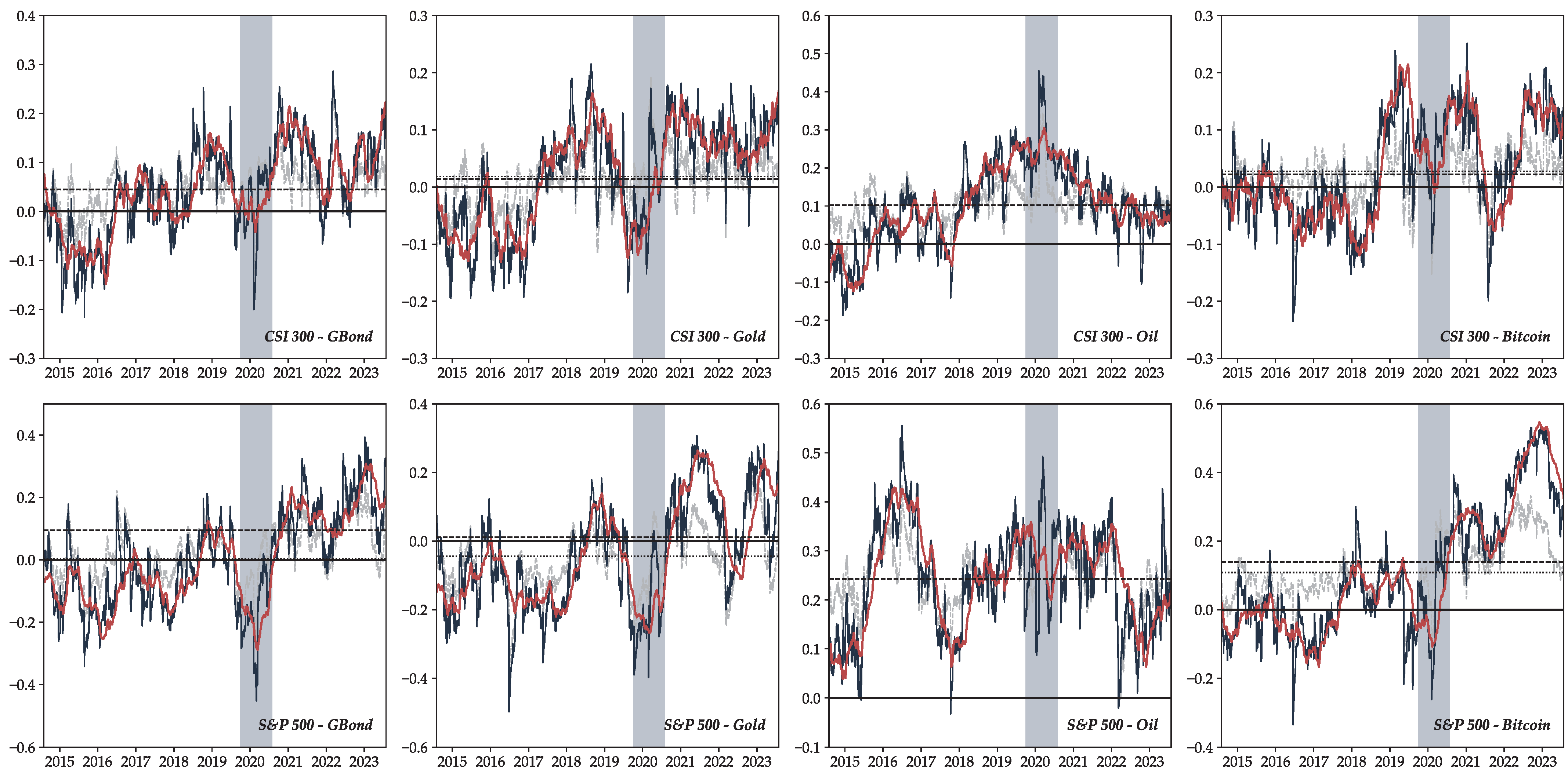
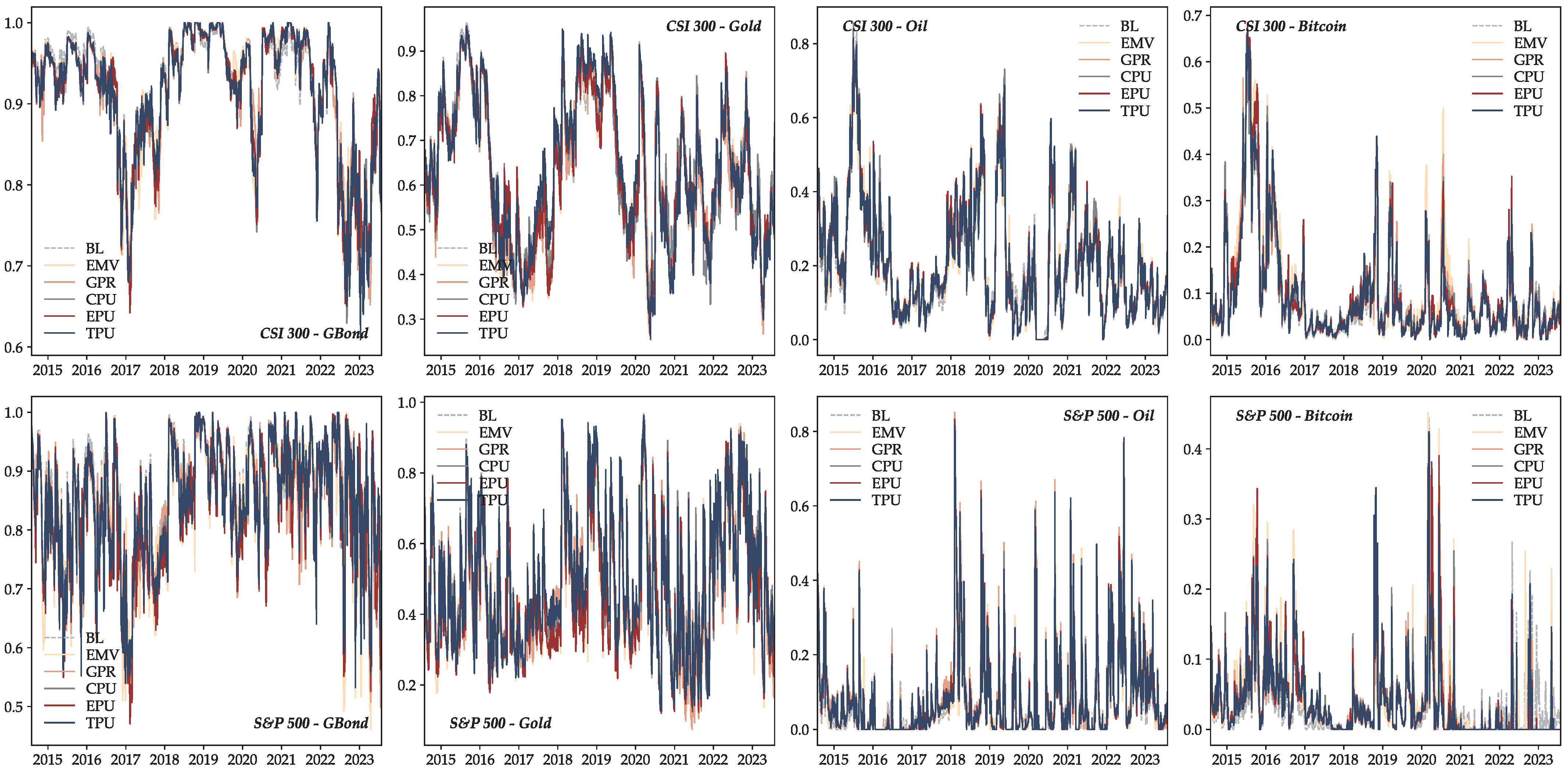
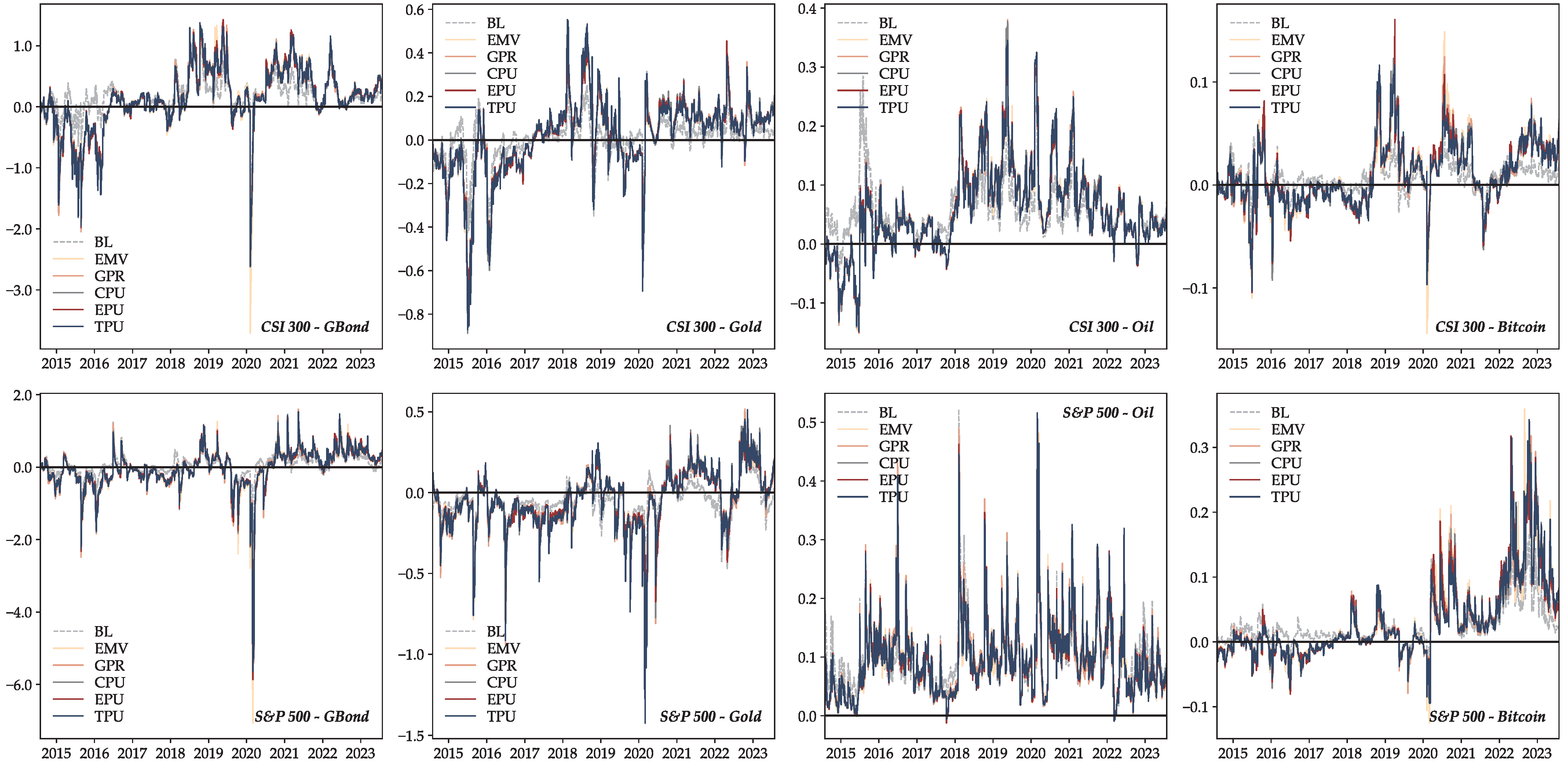
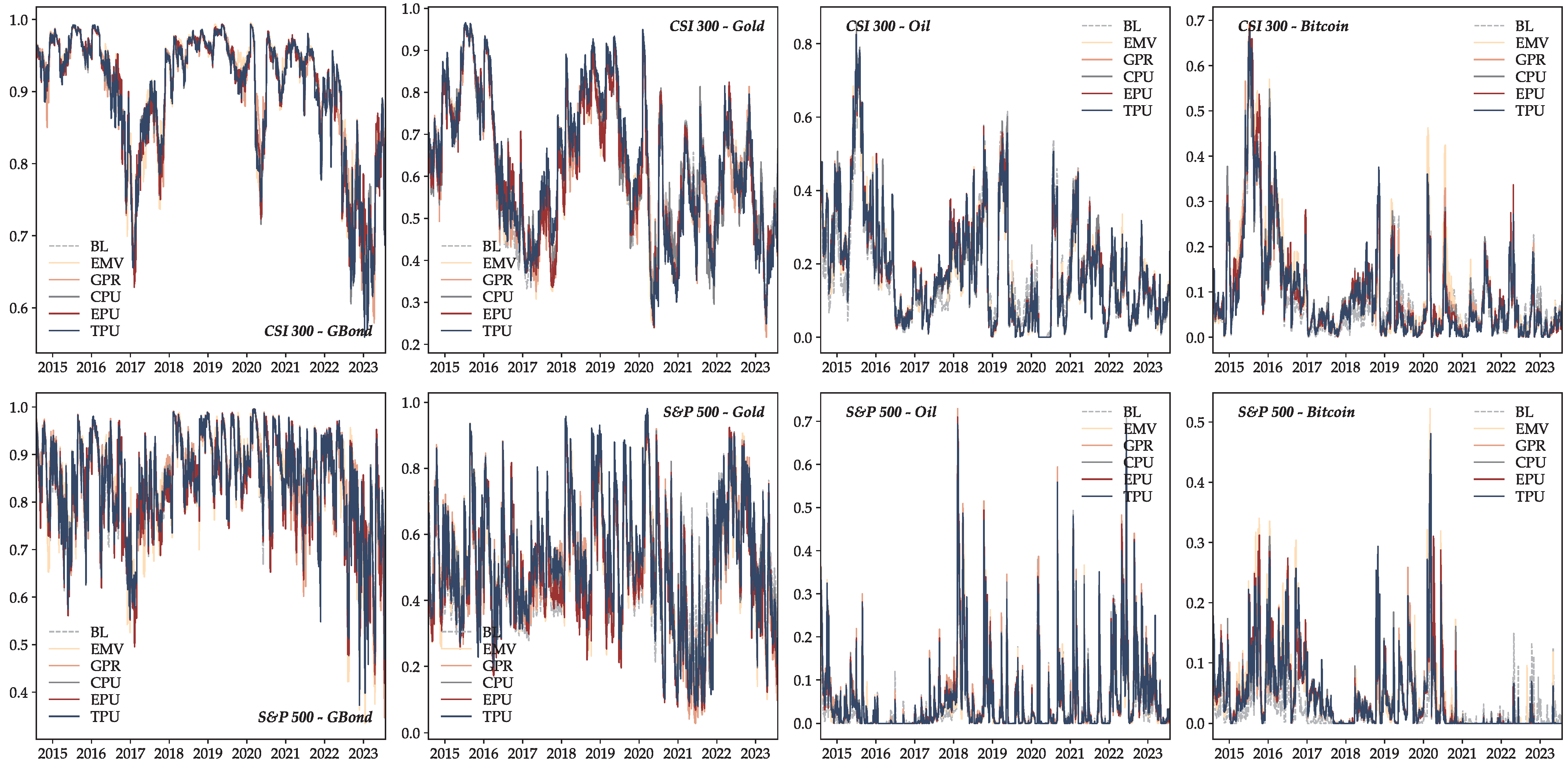
4.2. DCC-MIDAS Model Analysis
4.3. Risk Management Analysis
4.3.1. Optimal Weight and Hedge Ratio
4.3.2. Hedging Effectiveness
5. Conclusions
Author Contributions
Funding
Data Availability Statement
Conflicts of Interest
Appendix A

| CSI 300 | ||||||
| EPU | 0.0685 *** | 0.0113 | 0.9194 *** | −8.3393 *** | −8.2092 *** | 2.1651 *** |
| (0.0135) | (0.0201) | (0.0170) | (0.4171) | (0.5412) | (0.6939) | |
| CPU | 0.0730 *** | 0.0146 | 0.9100 *** | −8.3781 *** | −7.9229 *** | 1.0085 *** |
| (0.0142) | (0.0248) | (0.0207) | (0.3637) | (0.4792) | (0.2635) | |
| TPU | 0.0728 *** | 0.0100 | 0.9167 *** | −8.2424 *** | 1.3263 ** | 1.0011 *** |
| (0.0135) | (0.0222) | (0.0185) | (0.3989) | (0.6754) | (0.2711) | |
| EMV | 0.0720 *** | 0.0112 | 0.9166 *** | −8.2778 *** | −1.7397 *** | 3.0936 *** |
| (0.0134) | (0.0214) | (0.0175) | (0.3896) | (0.6639) | (1.1246) | |
| GPR | 0.0725 *** | 0.0064 | 0.9183 *** | −8.3142 *** | 2.8985 ** | 3.3888 *** |
| (0.0134) | (0.0204) | (0.0173) | (0.4098) | (1.4580) | (1.2977) | |
| S&P 500 | ||||||
| EPU | 0.0588 * | 0.2455 *** | 0.7952 *** | −8.7642 *** | −1.8095 *** | 22.8813 *** |
| (0.0312) | (0.0557) | (0.0352) | (0.4118) | (0.5265) | (0.4225) | |
| CPU | 0.0586 * | 0.2599 *** | 0.7844 *** | −8.8232 *** | 3.5732 *** | 1.0010 *** |
| (0.0333) | (0.0565) | (0.0368) | (0.4109) | (0.8432) | (0.3493) | |
| TPU | 0.0553 * | 0.2652 *** | 0.7782 *** | −8.8951 *** | −2.1221 *** | 1.9052 *** |
| (0.0334) | (0.0562) | (0.0366) | (0.3753) | (0.6562) | (0.7139) | |
| EMV | 0.0593 * | 0.2573 *** | 0.7859 *** | −8.8109 *** | −1.0351 *** | 21.0665 *** |
| (0.0324) | (0.0533) | (0.0345) | (0.3600) | (0.2698) | (2.6770) | |
| GPR | 0.0566 * | 0.2622 *** | 0.7821 *** | −8.8511 *** | −3.1628 *** | 2.7832 *** |
| (0.0338) | (0.0554) | (0.0371) | (0.3723) | (0.8383) | (0.9730) | |
| Green bond | ||||||
| EPU | 0.0497 *** | 0.0042 | 0.9409 *** | −11.1385 *** | −1.6032 *** | 2.5119 *** |
| (0.0190) | (0.0142) | (0.0166) | (0.3561) | (0.2722) | (0.4376) | |
| CPU | 0.0499 *** | 0.0039 | 0.9402 *** | −11.1669 *** | −0.5607 *** | 3.9462 *** |
| (0.0193) | (0.0140) | (0.0173) | (0.3119) | (0.1810) | (1.2879) | |
| TPU | 0.0533 *** | 0.0028 | 0.9391 *** | −11.1909 *** | −1.3696 ** | 1.0021 * |
| (0.0203) | (0.0141) | (0.0178) | (0.3487) | (0.5318) | (0.5201) | |
| EMV | 0.0487 ** | 0.0041 | 0.9417 *** | −11.1606 *** | 1.1281 *** | 1.9090 *** |
| (0.0195) | (0.0138) | (0.0171) | (0.3652) | (0.3792) | (0.4717) | |
| GPR | 0.0455 ** | 0.0060 | 0.9444 *** | −11.1678 *** | −0.3353 *** | 53.4786 *** |
| (0.0192) | (0.0134) | (0.0168) | (0.3692) | (0.0099) | (4.9185) | |
| Gold | ||||||
| EPU | 0.0291 ** | −0.0091 | 0.9682 *** | −9.2942 *** | −8.1935 *** | 1.0010 *** |
| (0.0130) | (0.0128) | (0.0135) | (0.2086) | (0.8913) | (0.2942) | |
| CPU | 0.0231 * | −0.0042 | 0.9733 *** | −9.2879 *** | −2.7295 *** | 1.1581 *** |
| (0.0124) | (0.0108) | (0.0174) | (0.2601) | (0.7121) | (0.2350) | |
| TPU | 0.0380 * | −0.0158 | 0.9471 *** | −9.3703 *** | −1.9933 * | 1.0010 *** |
| (0.0225) | (0.0222) | (0.0369) | (0.1097) | (1.0656) | (0.3732) | |
| EMV | 0.0400 * | −0.0178 | 0.9563 *** | −9.3444 *** | −5.8925 *** | 1.0010 ** |
| (0.0233) | (0.0215) | (0.0260) | (0.1617) | (1.4482) | (0.3919) | |
| GPR | 0.0261 * | −0.0056 | 0.9696 *** | −9.3300 *** | 4.7512 *** | 1.0010 ** |
| (0.0155) | (0.0123) | (0.0216) | (0.2622) | (0.6982) | (0.4045) | |
| Crude oil | ||||||
| EPU | 0.0482 *** | 0.1014 *** | 0.8871 *** | −7.2363 *** | −1.4578 *** | 16.6725 *** |
| (0.0162) | (0.0283) | (0.0203) | (0.3289) | (0.3032) | (2.7048) | |
| CPU | 0.0491 *** | 0.1015 *** | 0.8845 *** | −7.2648 *** | 1.8140 *** | 1.1171 ** |
| (0.0173) | (0.0304) | (0.0233) | (0.3255) | (0.6268) | (0.5207) | |
| TPU | 0.0510 *** | 0.1019 *** | 0.8819 *** | −7.2458 *** | −0.7394 *** | 2.1591 *** |
| (0.0178) | (0.0307) | (0.0239) | (0.3092) | (0.6502) | (0.3836) | |
| EMV | 0.0428 ** | 0.0970 *** | 0.8902 *** | −7.3414 *** | 10.8881 *** | 1.6725 *** |
| (0.0173) | (0.0306) | (0.0252) | (0.2814) | (0.6102) | (0.2242) | |
| GPR | 0.0451 *** | 0.1060 *** | 0.8845 *** | −7.3156 *** | 13.0378 *** | 1.2213 *** |
| (0.0172) | (0.0319) | (0.0255) | (0.3173) | (0.6495) | (0.3963) | |
| Bitcoin | ||||||
| EPU | 0.1365 *** | 0.0574 | 0.8008 *** | −5.3989 *** | −11.7293 *** | 2.5547 *** |
| (0.0447) | (0.0590) | (0.0495) | (0.5829) | (2.3877) | (0.8650) | |
| CPU | 0.1248 ** | 0.0546 | 0.8275 *** | −5.2172 *** | −4.9410 ** | 1.1463 ** |
| (0.0496) | (0.0525) | (0.0597) | (0.6587) | (1.9879) | (0.4782) | |
| TPU | 0.1153 ** | 0.0551 | 0.8350 *** | −5.3482 *** | −1.8477 ** | 2.8357 *** |
| (0.0513) | (0.0521) | (0.0707) | (0.6318) | (0.9120) | (0.7055) | |
| EMV | 0.1252 ** | 0.0464 | 0.8330 *** | −5.2446 *** | 0.7103 ** | 58.9370 *** |
| (0.0543) | (0.0485) | (0.0653) | (0.6366) | (0.2978) | (0.1654) | |
| GPR | 0.1113 ** | 0.0559 | 0.8431 *** | −5.2200 *** | −11.0058 *** | 1.0011 *** |
| (0.0448) | (0.0488) | (0.0563) | (0.6260) | (1.7109) | (0.2811) |
| Skewness | Kurtosis | J-B | L-B(10) | ARCH(10) | |
|---|---|---|---|---|---|
| CSI 300 | |||||
| EPU | −0.319 | 2.110 | 490.102 *** | 6.677 [0.671] | 3.884 [0.952] |
| CPU | −0.327 | 2.177 | 520.933 *** | 6.231 [0.717] | 4.311 [0.932] |
| TPU | −0.292 | 2.010 | 441.718 *** | 6.313 [0.708] | 3.959 [0.949] |
| EMV | −0.331 | 2.156 | 512.796 *** | 5.818 [0.758] | 4.516 [0.921] |
| GPR | −0.304 | 2.005 | 442.449 *** | 5.905 [0.749] | 4.245 [0.936] |
| Baseline | −0.295 | 1.942 | 415.250 *** | 6.087 [0.731] | 3.787 [0.956] |
| S&P 500 | |||||
| EPU | −0.688 | 2.741 | 947.981 *** | 8.866 [0.545] | 7.733 [0.655] |
| CPU | −0.791 | 2.995 | 1156.002 *** | 8.628 [0.568] | 6.808 [0.743] |
| TPU | −0.761 | 2.796 | 1021.092 *** | 8.745 [0.557] | 6.135 [0.804] |
| EMV | −0.741 | 2.644 | 925.753 *** | 8.741 [0.557] | 4.202 [0.938] |
| GPR | −0.744 | 2.648 | 929.553 *** | 7.461 [0.681] | 6.348 [0.785] |
| Baseline | −0.746 | 2.682 | 949.136 *** | 8.640 [0.567] | 6.310 [0.789] |
| GB | |||||
| EPU | −0.204 | 1.819 | 350.377 *** | 6.982 [0.727] | 6.814 [0.743] |
| CPU | −0.200 | 1.797 | 341.970 *** | 7.386 [0.689] | 7.118 [0.714] |
| TPU | −0.177 | 1.799 | 339.143 *** | 6.738 [0.750] | 6.512 [0.771] |
| EMV | −0.199 | 1.806 | 345.048 *** | 6.162 [0.724] | 9.756 [0.462] |
| GPR | −0.188 | 1.691 | 303.000 *** | 6.922 [0.733] | 6.931 [0.732] |
| Baseline | −0.197 | 1.752 | 325.459 *** | 6.087 [0.731] | 7.602 [0.668] |
| Gold | |||||
| EPU | −0.209 | 2.846 | 834.331 *** | 7.274 [0.699] | 3.459 [0.968] |
| CPU | −0.229 | 3.049 | 958.176 *** | 6.720 [0.752] | 4.766 [0.906] |
| TPU | −0.164 | 3.144 | 1006.818 *** | 6.885 [0.736] | 4.505 [0.922] |
| EMV | −0.167 | 2.994 | 914.855 *** | 6.256 [0.793] | 5.358 [0.866] |
| GPR | −0.138 | 2.806 | 801.156 *** | 6.783 [0.746] | 3.768 [0.957] |
| Baseline | −0.194 | 2.910 | 868.496 *** | 6.580 [0.764] | 3.433 [0.969] |
| Oil | |||||
| EPU | −0.427 | 2.962 | 957.572 *** | 8.376 [0.592] | 5.066 [0.887] |
| CPU | −0.460 | 3.048 | 1021.224 *** | 8.430 [0.587] | 5.366 [0.865] |
| TPU | −0.452 | 3.049 | 1019.080 *** | 8.378 [0.592] | 5.451 [0.859] |
| EMV | −0.485 | 2.791 | 879.832 *** | 8.396 [0.590] | 6.383 [0.782] |
| GPR | −0.446 | 2.922 | 940.659 *** | 8.697 [0.561] | 5.602 [0.847] |
| Baseline | −0.457 | 3.026 | 1006.829 *** | 8.160 [0.613] | 5.616 [0.846] |
| Bitcoin | |||||
| EPU | −0.073 | 9.394 | 8887.109 *** | 9.725 [0.465] | 9.239 [0.510] |
| CPU | −0.092 | 8.874 | 7931.548 *** | 8.349 [0.595] | 8.078 [0.621] |
| TPU | −0.239 | 9.494 | 9097.868 *** | 9.695 [0.468] | 9.209 [0.512] |
| EMV | −0.013 | 7.872 | 6239.620 *** | 9.670 [0.470] | 9.416 [0.493] |
| GPR | −0.118 | 8.042 | 6517.904 *** | 8.890 [0.543] | 8.583 [0.572] |
| Baseline | −0.058 | 7.307 | 5377.056 *** | 9.603 [0.476] | 8.652 [0.565] |
| S&P 500 | CSI 300 | |||||||
|---|---|---|---|---|---|---|---|---|
| Mean | Max. | Min. | Std. Dev. | Mean | Max. | Min. | Std. Dev. | |
| Panel: Short term | ||||||||
| GB | ||||||||
| EPU | 0.0052 | 0.3705 | −0.4578 | 0.1506 | 0.0444 | 0.2894 | −0.2200 | 0.0924 |
| CPU | 0.0037 | 0.3961 | −0.4631 | 0.1528 | 0.0441 | 0.3008 | −0.2301 | 0.0932 |
| TPU | 0.0048 | 0.3819 | −0.4566 | 0.1510 | 0.0446 | 0.2993 | −0.2279 | 0.0931 |
| EMV | 0.0027 | 0.3738 | −0.4730 | 0.1500 | 0.0440 | 0.2986 | −0.2648 | 0.0931 |
| GPR | 0.0031 | 0.3936 | −0.4526 | 0.1537 | 0.0444 | 0.2867 | −0.2153 | 0.0933 |
| Gold | ||||||||
| EPU | −0.0421 | 0.2909 | −0.4732 | 0.1530 | 0.0187 | 0.2105 | −0.1956 | 0.0930 |
| CPU | −0.0423 | 0.2929 | −0.4908 | 0.1553 | 0.0185 | 0.2117 | −0.2028 | 0.0938 |
| TPU | −0.0440 | 0.2871 | −0.4882 | 0.1531 | 0.0178 | 0.2121 | −0.2015 | 0.0937 |
| EMV | −0.0436 | 0.2815 | −0.4660 | 0.1504 | 0.0184 | 0.2020 | −0.1995 | 0.0923 |
| GPR | −0.0438 | 0.3078 | −0.4980 | 0.1566 | 0.0184 | 0.2154 | −0.1949 | 0.0933 |
| Oil | ||||||||
| EPU | 0.2411 | 0.5524 | −0.0513 | 0.1061 | 0.1025 | 0.4688 | −0.1795 | 0.1082 |
| CPU | 0.2428 | 0.5550 | −0.0359 | 0.1081 | 0.1031 | 0.4947 | −0.1857 | 0.1091 |
| TPU | 0.2424 | 0.5567 | −0.0297 | 0.1070 | 0.1028 | 0.4960 | −0.1814 | 0.1087 |
| EMV | 0.2430 | 0.5474 | −0.0131 | 0.1059 | 0.1030 | 0.4869 | −0.1791 | 0.1087 |
| GPR | 0.2421 | 0.5560 | −0.0331 | 0.1089 | 0.1027 | 0.4553 | −0.1870 | 0.1089 |
| Bitcoin | ||||||||
| EPU | 0.1087 | 0.5298 | −0.3230 | 0.1873 | 0.0294 | 0.2310 | −0.2121 | 0.0882 |
| CPU | 0.1084 | 0.5342 | −0.3207 | 0.1848 | 0.0291 | 0.2539 | −0.2195 | 0.0900 |
| TPU | 0.1080 | 0.5311 | −0.3349 | 0.1844 | 0.0292 | 0.2466 | −0.2265 | 0.0888 |
| EMV | 0.1067 | 0.5284 | −0.3281 | 0.1827 | 0.0273 | 0.2522 | −0.2308 | 0.0893 |
| GPR | 0.1083 | 0.5343 | −0.3352 | 0.1854 | 0.0274 | 0.2516 | −0.2352 | 0.0894 |
| Panel: Long term | ||||||||
| GB | ||||||||
| EPU | −0.0044 | 0.3083 | −0.2794 | 0.1396 | 0.0445 | 0.2215 | −0.1476 | 0.0800 |
| CPU | −0.0045 | 0.3087 | −0.2821 | 0.1404 | 0.0445 | 0.2193 | −0.1486 | 0.0801 |
| TPU | −0.0044 | 0.3090 | −0.2788 | 0.1397 | 0.0449 | 0.2206 | −0.1486 | 0.0799 |
| EMV | −0.0052 | 0.3051 | −0.2785 | 0.1393 | 0.0447 | 0.2226 | −0.1478 | 0.0799 |
| GPR | −0.0049 | 0.3085 | −0.2899 | 0.1409 | 0.0445 | 0.2232 | −0.1479 | 0.0801 |
| Gold | ||||||||
| EPU | −0.0378 | 0.2667 | −0.2626 | 0.1435 | 0.0196 | 0.1669 | −0.1318 | 0.0842 |
| CPU | −0.0378 | 0.2649 | −0.2666 | 0.1442 | 0.0202 | 0.1665 | −0.1328 | 0.0841 |
| TPU | −0.0385 | 0.2642 | −0.2648 | 0.1432 | 0.0198 | 0.1672 | −0.1324 | 0.0837 |
| EMV | −0.0382 | 0.2632 | −0.2647 | 0.1432 | 0.0202 | 0.1672 | −0.1332 | 0.0839 |
| GPR | −0.0383 | 0.2638 | −0.2672 | 0.1447 | 0.0201 | 0.1668 | −0.1310 | 0.0836 |
| Oil | ||||||||
| EPU | 0.2415 | 0.4340 | 0.0298 | 0.0959 | 0.1023 | 0.3043 | −0.1214 | 0.0987 |
| CPU | 0.2416 | 0.4311 | 0.0348 | 0.0966 | 0.1030 | 0.3048 | −0.1206 | 0.0985 |
| TPU | 0.2415 | 0.4331 | 0.0300 | 0.0961 | 0.1026 | 0.3049 | −0.1220 | 0.0987 |
| EMV | 0.2421 | 0.4355 | 0.0287 | 0.0963 | 0.1030 | 0.3059 | −0.1230 | 0.0990 |
| GPR | 0.2416 | 0.4293 | 0.0387 | 0.0970 | 0.1030 | 0.3049 | −0.1235 | 0.0990 |
| Bitcoin | ||||||||
| EPU | 0.1059 | 0.5557 | −0.1835 | 0.1852 | 0.0313 | 0.2162 | −0.1186 | 0.0870 |
| CPU | 0.1073 | 0.5515 | −0.1699 | 0.1842 | 0.0311 | 0.2167 | −0.1209 | 0.0870 |
| TPU | 0.1076 | 0.5546 | −0.1716 | 0.1831 | 0.0312 | 0.2155 | −0.1201 | 0.0864 |
| EMV | 0.1063 | 0.5534 | −0.1707 | 0.1821 | 0.0305 | 0.2126 | −0.1206 | 0.0864 |
| GPR | 0.1084 | 0.5467 | −0.1664 | 0.1836 | 0.0309 | 0.2144 | −0.1198 | 0.0869 |
| S&P 500 | CSI 300 | |||||||
|---|---|---|---|---|---|---|---|---|
| Mean | Max. | Min. | Std. Dev. | Mean | Max. | Min. | Std. Dev. | |
| Panel: Optimal weight | ||||||||
| GB | ||||||||
| EPU | 0.8392 | 1.0000 | 0.4709 | 0.1058 | 0.9132 | 1.0000 | 0.6421 | 0.0791 |
| CPU | 0.8443 | 1.0000 | 0.5403 | 0.0974 | 0.9134 | 1.0000 | 0.6293 | 0.0783 |
| TPU | 0.8439 | 1.0000 | 0.5320 | 0.0985 | 0.9131 | 1.0000 | 0.6090 | 0.0798 |
| EMV | 0.8475 | 1.0000 | 0.4616 | 0.1043 | 0.9156 | 1.0000 | 0.6450 | 0.0787 |
| GPR | 0.8441 | 1.0000 | 0.4983 | 0.1007 | 0.9144 | 1.0000 | 0.6520 | 0.0774 |
| Baseline | 0.8490 | 1.0000 | 0.5254 | 0.0960 | 0.9150 | 1.0000 | 0.6425 | 0.0788 |
| Gold | ||||||||
| EPU | 0.4693 | 0.9582 | 0.1200 | 0.1871 | 0.6262 | 0.9499 | 0.2543 | 0.1562 |
| CPU | 0.4787 | 0.9609 | 0.1374 | 0.1775 | 0.6323 | 0.9500 | 0.3085 | 0.1535 |
| TPU | 0.4876 | 0.9627 | 0.1245 | 0.1849 | 0.6394 | 0.9558 | 0.2591 | 0.1643 |
| EMV | 0.4757 | 0.9595 | 0.1356 | 0.1816 | 0.6272 | 0.9557 | 0.2758 | 0.1600 |
| GPR | 0.4733 | 0.9617 | 0.0752 | 0.1863 | 0.6264 | 0.9495 | 0.2667 | 0.1601 |
| Baseline | 0.4788 | 0.9716 | 0.1372 | 0.1790 | 0.6295 | 0.9630 | 0.2642 | 0.1579 |
| Oil | ||||||||
| EPU | 0.0790 | 0.8325 | 0.0000 | 0.1112 | 0.2169 | 0.8161 | 0.0000 | 0.1541 |
| CPU | 0.0765 | 0.8081 | 0.0000 | 0.1086 | 0.2133 | 0.8566 | 0.0000 | 0.1557 |
| TPU | 0.0777 | 0.8183 | 0.0000 | 0.1093 | 0.2147 | 0.8150 | 0.0000 | 0.1538 |
| EMV | 0.0768 | 0.8260 | 0.0000 | 0.1112 | 0.2117 | 0.7985 | 0.0000 | 0.1514 |
| GPR | 0.0804 | 0.8518 | 0.0000 | 0.1131 | 0.2162 | 0.8227 | 0.0000 | 0.1558 |
| Baseline | 0.0765 | 0.8479 | 0.0000 | 0.1115 | 0.2162 | 0.8501 | 0.0000 | 0.1560 |
| Bitcoin | ||||||||
| EPU | 0.0367 | 0.4217 | 0.0000 | 0.0574 | 0.0976 | 0.6841 | 0.0000 | 0.1168 |
| CPU | 0.0355 | 0.4062 | 0.0000 | 0.0532 | 0.0951 | 0.6082 | 0.0000 | 0.1057 |
| TPU | 0.0352 | 0.4244 | 0.0000 | 0.0529 | 0.0951 | 0.6670 | 0.0000 | 0.1108 |
| EMV | 0.0393 | 0.4523 | 0.0000 | 0.0589 | 0.1021 | 0.6637 | 0.0000 | 0.1212 |
| GPR | 0.0339 | 0.3826 | 0.0000 | 0.0476 | 0.0943 | 0.6464 | 0.0000 | 0.1065 |
| Baseline | 0.0324 | 0.4451 | 0.0000 | 0.0506 | 0.0981 | 0.6557 | 0.0000 | 0.1116 |
| Panel: Hedge ratio | ||||||||
| GB | ||||||||
| EPU | −0.0258 | 1.4091 | −5.8637 | 0.5422 | 0.1373 | 1.4284 | −2.5609 | 0.5013 |
| CPU | −0.0299 | 1.4756 | −5.7445 | 0.5523 | 0.1307 | 1.3166 | −2.6222 | 0.5016 |
| TPU | −0.0255 | 1.5261 | −5.6416 | 0.5414 | 0.1353 | 1.3785 | −2.6103 | 0.5050 |
| EMV | −0.0404 | 1.4183 | −7.0555 | 0.5784 | 0.1328 | 1.3849 | −3.7112 | 0.5310 |
| GPR | −0.0344 | 1.6044 | −5.8048 | 0.5525 | 0.1372 | 1.3342 | −2.1577 | 0.4937 |
| Baseline | 0.0476 | 1.2438 | −3.6794 | 0.3429 | 0.1768 | 1.1907 | −1.7684 | 0.2749 |
| Gold | ||||||||
| EPU | −0.0419 | 0.4543 | −1.1975 | 0.1702 | 0.0136 | 0.4757 | −0.8009 | 0.1680 |
| CPU | −0.0410 | 0.4753 | −1.1995 | 0.1765 | 0.0137 | 0.4879 | −0.8879 | 0.1744 |
| TPU | −0.0461 | 0.5119 | −1.4235 | 0.1813 | 0.0118 | 0.5528 | −0.8708 | 0.1803 |
| EMV | −0.0432 | 0.4545 | −1.3513 | 0.1728 | 0.0117 | 0.4599 | −0.8235 | 0.1697 |
| GPR | −0.0434 | 0.5167 | −1.1002 | 0.1749 | 0.0143 | 0.5347 | −0.7853 | 0.1686 |
| Baseline | −0.0507 | 0.4106 | −0.8170 | 0.1194 | 0.0076 | 0.3178 | −0.4260 | 0.0936 |
| Oil | ||||||||
| EPU | 0.0938 | 0.4859 | −0.0120 | 0.0605 | 0.0563 | 0.3340 | −0.1494 | 0.0699 |
| CPU | 0.0939 | 0.5161 | −0.0089 | 0.0607 | 0.0559 | 0.3775 | −0.1465 | 0.0711 |
| TPU | 0.0941 | 0.5160 | −0.0089 | 0.0607 | 0.0559 | 0.3453 | −0.1484 | 0.0706 |
| EMV | 0.0940 | 0.5073 | −0.0040 | 0.0603 | 0.0552 | 0.3518 | −0.1506 | 0.0697 |
| GPR | 0.0942 | 0.4902 | −0.0089 | 0.0620 | 0.0563 | 0.3805 | −0.1513 | 0.0713 |
| Baseline | 0.0960 | 0.5226 | −0.0031 | 0.0548 | 0.0581 | 0.2843 | −0.0596 | 0.0452 |
| Bitcoin | ||||||||
| EPU | 0.0307 | 0.3176 | −0.0876 | 0.0588 | 0.0106 | 0.1605 | −0.1045 | 0.0299 |
| CPU | 0.0301 | 0.3079 | −0.0881 | 0.0576 | 0.0105 | 0.1500 | −0.0991 | 0.0307 |
| TPU | 0.0296 | 0.3426 | −0.0949 | 0.0584 | 0.0101 | 0.1166 | −0.1027 | 0.0295 |
| EMV | 0.0301 | 0.3591 | −0.1247 | 0.0592 | 0.0096 | 0.1488 | −0.1440 | 0.0319 |
| GPR | 0.0294 | 0.3179 | −0.0795 | 0.0574 | 0.0101 | 0.1375 | −0.0964 | 0.0296 |
| Baseline | 0.0288 | 0.2230 | −0.0458 | 0.0338 | 0.0079 | 0.0808 | −0.0841 | 0.0164 |
| S&P 500 | CSI 300 | |||||||||
|---|---|---|---|---|---|---|---|---|---|---|
| Mean | Max. | Min. | Std. Dev. | t-Statistic | Mean | Max. | Min. | Std. Dev. | t-Statistic | |
| Panel: Diversified portfolio | ||||||||||
| GB | ||||||||||
| EPU | 0.8332 | 0.9960 | 0.3765 | 0.1105 | −70.652 *** | 0.8990 | 0.9934 | 0.5902 | 0.0865 | −54.679 *** |
| CPU | 0.8389 | 0.9960 | 0.3776 | 0.1016 | −74.265 *** | 0.8992 | 0.9931 | 0.5910 | 0.0858 | −55.022 *** |
| TPU | 0.8381 | 0.9960 | 0.3725 | 0.1030 | −73.556 *** | 0.8987 | 0.9932 | 0.5592 | 0.0879 | −53.910 *** |
| EMV | 0.8423 | 0.9967 | 0.3349 | 0.1094 | −67.477 *** | 0.9015 | 0.9955 | 0.5933 | 0.0871 | −52.934 *** |
| GPR | 0.8387 | 0.9958 | 0.3459 | 0.1062 | −71.116 *** | 0.9001 | 0.9924 | 0.5790 | 0.0858 | −54.507 *** |
| Baseline | 0.8382 | 0.9960 | 0.4122 | 0.1002 | −75.607 *** | 0.9007 | 0.9932 | 0.6089 | 0.0845 | −55.002 *** |
| Gold | ||||||||||
| EPU | 0.4916 | 0.9784 | 0.0672 | 0.1928 | −123.440 *** | 0.6159 | 0.9620 | 0.2396 | 0.1612 | −111.557 *** |
| CPU | 0.5008 | 0.9799 | 0.0784 | 0.1824 | −128.142 *** | 0.6220 | 0.9645 | 0.2633 | 0.1572 | −112.524 *** |
| TPU | 0.5104 | 0.9812 | 0.0800 | 0.1904 | −120.364 *** | 0.6295 | 0.9658 | 0.2459 | 0.1696 | −102.250 *** |
| EMV | 0.4983 | 0.9796 | 0.0893 | 0.1869 | −125.656 *** | 0.6169 | 0.9646 | 0.2263 | 0.1653 | −108.508 *** |
| GPR | 0.4972 | 0.9803 | 0.0283 | 0.1919 | −122.626 *** | 0.6162 | 0.9616 | 0.2170 | 0.1648 | −109.005 *** |
| Baseline | 0.5027 | 0.9804 | 0.1077 | 0.1777 | −131.028 *** | 0.6231 | 0.9648 | 0.2449 | 0.1615 | −109.213 *** |
| Oil | ||||||||||
| EPU | 0.0501 | 0.7097 | 0.0000 | 0.0846 | −525.330 *** | 0.1879 | 0.8255 | 0.0000 | 0.1489 | −255.278 *** |
| CPU | 0.0484 | 0.6855 | 0.0000 | 0.0822 | −542.040 *** | 0.1847 | 0.8573 | 0.0000 | 0.1511 | −252.579 *** |
| TPU | 0.0490 | 0.6939 | 0.0000 | 0.0831 | −535.887 *** | 0.1860 | 0.8249 | 0.0000 | 0.1493 | −255.220 *** |
| EMV | 0.0488 | 0.7067 | 0.0000 | 0.0852 | −522.650 *** | 0.1831 | 0.8179 | 0.0000 | 0.1471 | −259.990 *** |
| GPR | 0.0517 | 0.7297 | 0.0000 | 0.0865 | −513.176 *** | 0.1874 | 0.8261 | 0.0000 | 0.1508 | −252.191 *** |
| Baseline | 0.0448 | 0.7088 | 0.0000 | 0.0833 | −536.951 *** | 0.1828 | 0.8114 | 0.0000 | 0.1454 | −263.056 *** |
| Bitcoin | ||||||||||
| EPU | 0.0399 | 0.4740 | 0.0000 | 0.0603 | −745.328 *** | 0.0953 | 0.6948 | 0.0000 | 0.1177 | −359.681 *** |
| CPU | 0.0387 | 0.4608 | 0.0000 | 0.0572 | −786.952 *** | 0.0930 | 0.6426 | 0.0000 | 0.1070 | −396.644 *** |
| TPU | 0.0387 | 0.4808 | 0.0000 | 0.0587 | −766.538 *** | 0.0932 | 0.6768 | 0.0000 | 0.1123 | −377.923 *** |
| EMV | 0.0418 | 0.5225 | 0.0000 | 0.0635 | −706.105 *** | 0.1005 | 0.6904 | 0.0000 | 0.1232 | −341.629 *** |
| GPR | 0.0374 | 0.3960 | 0.0000 | 0.0538 | −837.241 *** | 0.0925 | 0.6574 | 0.0000 | 0.1076 | −394.870 *** |
| Baseline | 0.0241 | 0.4471 | 0.0000 | 0.0441 | −1034.793 *** | 0.0935 | 0.6534 | 0.0000 | 0.1101 | −385.391 *** |
| Panel: Hedging portfolio | ||||||||||
| GB | ||||||||||
| EPU | 0.0227 | 0.2095 | 0.0000 | 0.0271 | −1689.109 *** | 0.0105 | 0.0838 | 0.0000 | 0.0120 | −3851.773 *** |
| CPU | 0.0233 | 0.2144 | 0.0000 | 0.0280 | −1630.750 *** | 0.0106 | 0.0905 | 0.0000 | 0.0123 | −3760.641 *** |
| TPU | 0.0228 | 0.2085 | 0.0000 | 0.0276 | −1659.759 *** | 0.0107 | 0.0896 | 0.0000 | 0.0124 | −3747.663 *** |
| EMV | 0.0225 | 0.2237 | 0.0000 | 0.0272 | −1684.056 *** | 0.0106 | 0.0892 | 0.0000 | 0.0123 | −3755.614 *** |
| GPR | 0.0236 | 0.2048 | 0.0000 | 0.0281 | −1626.581 *** | 0.0107 | 0.0822 | 0.0000 | 0.0121 | −3841.412 *** |
| Baseline | 0.0085 | 0.0791 | 0.0000 | 0.0118 | −3931.693 *** | 0.0051 | 0.0652 | 0.0000 | 0.0067 | −6941.402 *** |
| Gold | ||||||||||
| EPU | 0.0252 | 0.2240 | 0.0000 | 0.0284 | −1603.897 *** | 0.0090 | 0.0443 | 0.0000 | 0.0085 | −5489.032 *** |
| CPU | 0.0259 | 0.2408 | 0.0000 | 0.0296 | −1539.483 *** | 0.0091 | 0.0448 | 0.0000 | 0.0087 | −5334.586 *** |
| TPU | 0.0254 | 0.2383 | 0.0000 | 0.0293 | −1556.556 *** | 0.0091 | 0.0450 | 0.0000 | 0.0086 | −5376.640 *** |
| EMV | 0.0245 | 0.2172 | 0.0000 | 0.0281 | −1626.047 *** | 0.0089 | 0.0408 | 0.0000 | 0.0083 | −5615.465 *** |
| GPR | 0.0264 | 0.2480 | 0.0000 | 0.0301 | −1514.439 *** | 0.0090 | 0.0464 | 0.0000 | 0.0086 | −5365.987 *** |
| Baseline | 0.0113 | 0.1517 | 0.0000 | 0.0166 | −2785.107 *** | 0.0024 | 0.0370 | 0.0000 | 0.0036 | −13085.813 *** |
| Oil | ||||||||||
| EPU | 0.0694 | 0.3052 | 0.0000 | 0.0534 | −815.887 *** | 0.0222 | 0.2198 | 0.0000 | 0.0296 | −1544.519 *** |
| CPU | 0.0706 | 0.3081 | 0.0000 | 0.0546 | −796.502 *** | 0.0225 | 0.2447 | 0.0000 | 0.0308 | −1484.160 *** |
| TPU | 0.0702 | 0.3099 | 0.0000 | 0.0542 | −803.216 *** | 0.0224 | 0.2460 | 0.0000 | 0.0305 | −1500.522 *** |
| EMV | 0.0702 | 0.2996 | 0.0000 | 0.0537 | −810.347 *** | 0.0224 | 0.2371 | 0.0000 | 0.0303 | −1509.488 *** |
| GPR | 0.0705 | 0.3091 | 0.0000 | 0.0545 | −798.197 *** | 0.0224 | 0.2073 | 0.0000 | 0.0295 | −1552.297 *** |
| Baseline | 0.0651 | 0.2188 | 0.0000 | 0.0339 | −1290.985 *** | 0.0136 | 0.1480 | 0.0000 | 0.0153 | −3014.941 *** |
| Bitcoin | ||||||||||
| EPU | 0.0469 | 0.2807 | 0.0000 | 0.0695 | −642.251 *** | 0.0086 | 0.0534 | 0.0000 | 0.0095 | −4867.274 *** |
| CPU | 0.0459 | 0.2854 | 0.0000 | 0.0688 | −649.241 *** | 0.0089 | 0.0644 | 0.0000 | 0.0103 | −4509.391 *** |
| TPU | 0.0457 | 0.2820 | 0.0000 | 0.0684 | −652.881 *** | 0.0087 | 0.0608 | 0.0000 | 0.0101 | −4605.092 *** |
| EMV | 0.0447 | 0.2792 | 0.0000 | 0.0666 | −671.739 *** | 0.0087 | 0.0636 | 0.0000 | 0.0101 | −4591.221 *** |
| GPR | 0.0461 | 0.2854 | 0.0000 | 0.0690 | −647.428 *** | 0.0087 | 0.0633 | 0.0000 | 0.0103 | −4524.398 *** |
| Baseline | 0.0218 | 0.1151 | 0.0000 | 0.0247 | −1856.221 *** | 0.0027 | 0.0233 | 0.0000 | 0.0033 | −14223.883 *** |
| S&P 500 | CSI 300 | |||||||||||
|---|---|---|---|---|---|---|---|---|---|---|---|---|
| EPU | CPU | TPU | EMV | GPR | Baseline | EPU | CPU | TPU | EMV | GPR | Baseline | |
| Panel: Diversified portfolio | ||||||||||||
| VaR reduction | ||||||||||||
| GB | 0.6969 | 0.6964 | 0.6963 | 0.6956 | 0.6970 | 0.6967 | 0.7583 | 0.7586 | 0.7586 | 0.7583 | 0.7584 | 0.7584 |
| Gold | 0.4524 | 0.4530 | 0.4534 | 0.4526 | 0.4543 | 0.4523 | 0.5121 | 0.5117 | 0.5110 | 0.5132 | 0.5126 | 0.5112 |
| Oil | −0.0533 | −0.0516 | −0.0494 | −0.0519 | −0.0666 | −0.0563 | 0.1670 | 0.1692 | 0.1690 | 0.1701 | 0.1703 | 0.1654 |
| Bitcoin | −0.0539 | −0.0465 | −0.0556 | −0.0393 | −0.0327 | −0.0562 | 0.1494 | 0.1482 | 0.1473 | 0.1561 | 0.1519 | 0.1505 |
| ES reduction | ||||||||||||
| GB | 0.7042 | 0.7050 | 0.7055 | 0.7050 | 0.7022 | 0.7033 | 0.7801 | 0.7817 | 0.7817 | 0.7807 | 0.7808 | 0.7797 |
| Gold | 0.4801 | 0.4800 | 0.4878 | 0.4831 | 0.4819 | 0.4860 | 0.5609 | 0.5585 | 0.5617 | 0.5634 | 0.5664 | 0.5618 |
| Oil | −0.1510 | −0.1506 | −0.1292 | −0.1313 | −0.1764 | −0.1544 | 0.1882 | 0.1944 | 0.1959 | 0.1930 | 0.1924 | 0.1831 |
| Bitcoin | −0.1136 | −0.0979 | −0.1161 | −0.0700 | −0.0760 | −0.1155 | 0.1919 | 0.1823 | 0.1814 | 0.1980 | 0.1879 | 0.1784 |
| LPM reduction | ||||||||||||
| GB | 0.6450 | 0.6446 | 0.6446 | 0.6437 | 0.6453 | 0.6440 | 0.7266 | 0.7271 | 0.7272 | 0.7269 | 0.7271 | 0.7268 |
| Gold | 0.3910 | 0.3924 | 0.3918 | 0.3914 | 0.3937 | 0.3912 | 0.4596 | 0.4595 | 0.4590 | 0.4597 | 0.4602 | 0.4591 |
| Oil | −0.0342 | −0.0318 | −0.0306 | −0.0343 | −0.0370 | −0.0320 | 0.0898 | 0.0900 | 0.0897 | 0.0898 | 0.0910 | 0.0894 |
| Bitcoin | −0.0434 | −0.0416 | −0.0425 | −0.0331 | −0.0384 | −0.0407 | 0.0869 | 0.0837 | 0.0827 | 0.0910 | 0.0842 | 0.0866 |
| Panel: Hedging portfolio | ||||||||||||
| VaR reduction | ||||||||||||
| GB | −0.0359 | −0.0331 | −0.0328 | −0.0463 | −0.0356 | −0.0003 | 0.0372 | 0.0376 | 0.0378 | 0.0372 | 0.0379 | 0.0358 |
| Gold | −0.0093 | −0.0081 | −0.0139 | −0.0135 | −0.0042 | 0.0157 | 0.0367 | 0.0374 | 0.0365 | 0.0371 | 0.0373 | 0.0369 |
| Oil | 0.0540 | 0.0556 | 0.0541 | 0.0579 | 0.0584 | 0.0600 | 0.0430 | 0.0431 | 0.0429 | 0.0434 | 0.0432 | 0.0491 |
| Bitcoin | 0.0691 | 0.0652 | 0.0655 | 0.0580 | 0.0601 | 0.0701 | 0.0298 | 0.0303 | 0.0308 | 0.0296 | 0.0308 | 0.0332 |
| ES reduction | ||||||||||||
| GB | −0.0832 | −0.0764 | −0.0772 | −0.0962 | −0.0782 | −0.0013 | 0.0072 | 0.0076 | 0.0078 | 0.0030 | 0.0161 | 0.0093 |
| Gold | −0.0171 | −0.0157 | −0.0342 | −0.0335 | −0.0077 | 0.0149 | 0.0196 | 0.0198 | 0.0193 | 0.0196 | 0.0206 | 0.0192 |
| Oil | 0.0694 | 0.0725 | 0.0717 | 0.0792 | 0.0781 | 0.0690 | −0.0076 | −0.0121 | −0.0123 | −0.0126 | −0.0075 | 0.0078 |
| Bitcoin | 0.0697 | 0.0603 | 0.0560 | 0.0507 | 0.0533 | 0.0795 | 0.0027 | 0.0028 | −0.0047 | −0.0070 | −0.0053 | −0.0079 |
| LPM reduction | ||||||||||||
| GB | −0.0299 | −0.0273 | −0.0278 | −0.0327 | −0.0284 | −0.0274 | −0.0099 | −0.0092 | −0.0091 | −0.0098 | −0.0097 | −0.0073 |
| Gold | −0.0351 | −0.0329 | −0.0360 | −0.0368 | −0.0304 | −0.0286 | −0.0057 | −0.0050 | −0.0061 | −0.0054 | −0.0053 | −0.0051 |
| Oil | 0.0139 | 0.0156 | 0.0147 | 0.0171 | 0.0180 | 0.0174 | −0.0004 | −0.0009 | −0.0007 | 0.0000 | −0.0010 | 0.0042 |
| Bitcoin | 0.0020 | −0.0012 | 0.0010 | −0.0057 | 0.0011 | −0.0057 | −0.0161 | −0.0151 | −0.0141 | −0.0169 | −0.0149 | −0.0101 |
References
- Akhtaruzzaman, Md, Sabri Boubaker, Brian M. Lucey, and Ahmet Sensoy. 2021. Is gold a hedge or a safe-haven asset in the COVID–19 crisis? Economic Modelling 102: 105588. [Google Scholar] [CrossRef]
- Al Mamun, Md, Gazi Salah Uddin, Muhammad Tahir Suleman, and Sang Hoon Kang. 2020. Geopolitical risk, uncertainty and Bitcoin Investment. Physica A: Statistical Mechanics and Its Applications 540: 123107. [Google Scholar] [CrossRef]
- Amendola, Alessandra, Vincenzo Candila, and Giampiero M. Gallo. 2019. On the asymmetric impact of macro–variables on volatility. Economic Modelling 76: 135–52. [Google Scholar] [CrossRef]
- Amendola, Alessandra, Vincenzo Candila, and Giampiero M. Gallo. 2020. Choosing between weekly and monthly volatility drivers within a double asymmetric GARCH-Midas model. In Springer Proceedings in Mathematics & Statistics. Berlin/Heidelberg: Springer, pp. 25–34. [Google Scholar] [CrossRef]
- Amendola, Alessandra, Vincenzo Candila, and Giampiero M. Gallo. 2021. Choosing the frequency of volatility components within the double asymmetric GARCH–midas–X model. Econometrics and Statistics 20: 12–28. [Google Scholar] [CrossRef]
- Artzner, Philippe. 1997. Thinking coherently. Risk 10: 68–71. [Google Scholar]
- Baker, Scott R., Nicholas Bloom, and Steven J. Davis. 2016. Measuring economic policy uncertainty. The Quarterly Journal of Economics 131: 1593–1636. [Google Scholar] [CrossRef]
- Baker, Scott R, Nicholas Bloom, Steven J. Davis, and Kyle J. Kost. 2019. Policy News and Stock Market Volatility. Cambridge: National Bureau of Economic Research. [Google Scholar] [CrossRef]
- Bawa, Vijay S. 1975. Optimal rules for ordering uncertain prospects. Journal of Financial Economics 2: 95–121. [Google Scholar] [CrossRef]
- Bellard, Céline, Cleo Bertelsmeier, Paul Leadley, Wilfried Thuiller, and Franck Courchamp. 2012. Impacts of climate change on the future of Biodiversity. Ecology Letters 15: 365–77. [Google Scholar] [CrossRef]
- Ben Nouir, Jihed, and Hayet Ben Haj Hamida. 2023. How do economic policy uncertainty and geopolitical risk drive bitcoin volatility? Research in International Business and Finance 64: 101809. [Google Scholar] [CrossRef]
- Bollerslev, Tim. 1986. Generalized autoregressive conditional heteroskedasticity. Journal of Econometrics 31: 307–27. [Google Scholar] [CrossRef]
- Boufounou, Paraskevi, and Dimitrios Tinos. 2023. Stock markets integration perspectives towards sustainable finance: Evidence of developed and Emerging Financial Markets. Reference Module in Social Sciences. [Google Scholar] [CrossRef]
- Butt, Hilal Anwar, Riza Demirer, Mohsin Sadaqat, and Muhammad Tahir Suleman. 2022. Do emerging stock markets offer an illiquidity premium for local or global investors? The Quarterly Review of Economics and Finance 86: 502–15. [Google Scholar] [CrossRef]
- Caldara, Dario, and Matteo Iacoviello. 2022. Measuring geopolitical risk. American Economic Review 112: 1194–1225. [Google Scholar] [CrossRef]
- Cao, Yan, Sheng Cheng, and Xinran Li. 2023. How economic policy uncertainty affects asymmetric spillovers in food and oil prices: Evidence from wavelet analysis. Resources Policy 86: 104086. [Google Scholar] [CrossRef]
- Cheng, Hui-Pei, and Kuang-Chieh Yen. 2020. The relationship between the economic policy uncertainty and the cryptocurrency market. Finance Research Letters 35: 101308. [Google Scholar] [CrossRef]
- Cheng, Sheng, Zongyou Zhang, and Yan Cao. 2022. Can precious metals hedge geopolitical risk? fresh sight using wavelet coherence analysis. Resources Policy 79: 102972. [Google Scholar] [CrossRef]
- Chen, Jinyu, Yuxin Huang, Xiaohang Ren, and Jingxiao Qu. 2022. Time-varying spillovers between trade policy uncertainty and precious metal markets: Evidence from China-US trade conflict. Resources Policy 76: 102577. [Google Scholar] [CrossRef]
- Chen, Yong, Jing Fang, and Dingming Liu. 2023. The effects of Trump’s Trade War on U.S. Financial Markets. Journal of International Money and Finance 134: 102842. [Google Scholar] [CrossRef]
- Colacito, Riccardo, Robert F. Engle, and Eric Ghysels. 2011. A component model for dynamic correlations. Journal of Econometrics 164: 45–59. [Google Scholar] [CrossRef]
- Conrad, Christian, Karin Loch, and Daniel Rittler. 2014. On the macroeconomic determinants of long-term volatilities and correlations in U.S. stock and crude oil markets. Journal of Empirical Finance 29: 26–40. [Google Scholar] [CrossRef]
- Cotter, John, and Jim Hanly. 2012. Hedging effectiveness under conditions of asymmetry. The European Journal of Finance 18: 135–47. [Google Scholar] [CrossRef]
- Dai, Zhifeng, Haoyang Zhu, and Xinhua Zhang. 2022. Dynamic spillover effects and portfolio strategies between crude oil, gold and Chinese stock markets related to New Energy Vehicle. Energy Economics 109: 105959. [Google Scholar] [CrossRef]
- Ding, Hao, Qiang Ji, Rufei Ma, and Pengxiang Zhai. 2022. High-Carbon Screening Out: A DCC-Midas-Climate Policy Risk Method. Finance Research Letters 47: 102818. [Google Scholar] [CrossRef]
- Dong, Xiyong, Youlin Xiong, Siyue Nie, and Seong-Min Yoon. 2023. Can bonds hedge stock market risks? green bonds vs conventional bonds. Finance Research Letters 52: 103367. [Google Scholar] [CrossRef]
- Engle, Robert F., Eric Ghysels, and Bumjean Sohn. 2013. Stock market volatility and macroeconomic fundamentals. Review of Economics and Statistics 95: 776–97. [Google Scholar] [CrossRef]
- Garcia-Jorcano, Laura, and Sonia Benito. 2020. Studying the properties of the Bitcoin as a diversifying and hedging asset through a copula analysis: Constant and time-varying. Research in International Business and Finance 54: 101300. [Google Scholar] [CrossRef] [PubMed]
- Gavriilidis, Konstantinos. 2021. Measuring climate policy uncertainty. SSRN Electronic Journal. [Google Scholar] [CrossRef]
- Glosten, Lawrence R., Ravi Jagannathan, and David Edward Runkle. 1993. On the Relation between the Expected Value and the Volatility of the Nominal Excess Return on Stocks. The Journal of Finance 48: 1779–1801. [Google Scholar] [CrossRef]
- Godil, Danish Iqbal, Salman Sarwat, Arshian Sharif, and Kittisak Jermsittiparsert. 2020. How oil prices, gold prices, uncertainty and risk impact Islamic and conventional stocks? empirical evidence from QARDL technique. Resources Policy 66: 101638. [Google Scholar] [CrossRef]
- Guo, Dong, and Peng Zhou. 2021. Green bonds as hedging assets before and after COVID: A comparative study between the US and China. Energy Economics 104: 105696. [Google Scholar] [CrossRef]
- Hamma, Wajdi, Ahmed Ghorbel, and Anis Jarboui. 2021. Hedging islamic and conventional stock markets with other financial assets: Comparison between competing DCC models on hedging effectiveness. Journal of Asset Management 22: 179–99. [Google Scholar] [CrossRef]
- Hasan, Md. Bokhtiar, M. Kabir Hassan, Zeynullah Gider, Humaira Tahsin Rafia, and Mamunur Rashid. 2023. Searching hedging instruments against diverse global risks and uncertainties. The North American Journal of Economics and Finance 66: 101893. [Google Scholar] [CrossRef]
- Jin, Jiayu, Liyan Han, Lei Wu, and Hongchao Zeng. 2020. The hedging effect of green bonds on carbon market risk. International Review of Financial Analysis 71: 101509. [Google Scholar] [CrossRef]
- Kamal, Javed Bin, Mark Wohar, and Khaled Bin Kamal. 2022. Do gold, oil, equities, and currencies hedge economic policy uncertainty and geopolitical risks during Covid Crisis? Resources Policy 78: 102920. [Google Scholar] [CrossRef]
- Korotin, Vladimir, Maxim Dolgonosov, Victor Popov, Olesya Korotina, and Inna Korolkova. 2019. The Ukrainian crisis, economic sanctions, oil shock and commodity currency: Analysis based on EMD approach. Research in International Business and Finance 48: 156–68. [Google Scholar] [CrossRef]
- Kroner, Kenneth F., and Jahangir Sultan. 1993. Time-varying distributions and dynamic hedging with foreign currency futures. The Journal of Financial and Quantitative Analysis 28: 535. [Google Scholar] [CrossRef]
- Kroner, Kenneth F., and Victor K. Ng. 1998. Modeling asymmetric comovements of asset returns. Review of Financial Studies 11: 817–44. [Google Scholar] [CrossRef]
- Ku, Yuan-Hung Hsu, Ho-Chyuan Chen, and Kuang-Hua Chen. 2007. On the application of the dynamic conditional correlation model in estimating optimal time-varying hedge ratios. Applied Economics Letters 14: 503–9. [Google Scholar] [CrossRef]
- Lin, Ling, Zhongbao Zhou, Yong Jiang, and Yangchen Ou. 2021. Risk spillovers and hedge strategies between global crude oil markets and stock markets: Do regime switching processes combining long memory and asymmetry matter? The North American Journal of Economics and Finance 57: 101398. [Google Scholar] [CrossRef]
- Ma, Rufei, Bianxia Sun, Pengxiang Zhai, and Yi Jin. 2021. Hedging stock market risks: Can gold really beat bonds? Finance Research Letters 42: 101918. [Google Scholar] [CrossRef]
- Mensi, Walid, Md Rajib Kamal, Xuan Vinh Vo, and Sang Hoon Kang. 2023. Extreme dependence and spillovers between uncertainty indices and stock markets: Does the US market play a major role? The North American Journal of Economics and Finance 68: 101970. [Google Scholar] [CrossRef]
- Meyer, Klaus E., Tony Fang, Andrei Y. Panibratov, Mike W. Peng, and Ajai Gaur. 2023. International Business Under Sanctions. Journal of World Business 58: 101426. [Google Scholar] [CrossRef]
- Reboredo, Juan C. 2018. Green bond and financial markets: Co-movement, diversification and price spillover effects. Energy Economics 74: 38–50. [Google Scholar] [CrossRef]
- Saâdaoui, Foued, Sami Ben Jabeur, and John W. Goodell. 2022. Causality of geopolitical risk on food prices: Considering the russo–ukrainian conflict. Finance Research Letters 49: 103103. [Google Scholar] [CrossRef]
- Salisu, Afees A., Ahamuefula E. Ogbonna, Lukman Lasisi, and Abeeb Olaniran. 2022. Geopolitical risk and stock market volatility in emerging markets: A GARCH—Midas approach. The North American Journal of Economics and Finance 62: 101755. [Google Scholar] [CrossRef]
- Simran, and Anil Kumar Sharma. 2023. Asymmetric impact of economic policy uncertainty on cryptocurrency market: Evidence from NARDL approach. The Journal of Economic Asymmetries 27: e00298. [Google Scholar] [CrossRef]
- Umar, Zaghum, Ahmed Bossman, Sun-Yong Choi, and Xuan Vinh Vo. 2023. Are short stocks susceptible to geopolitical shocks? time-frequency evidence from the Russian-ukrainian conflict. Finance Research Letters 52: 103388. [Google Scholar] [CrossRef]
- Xiang, Feiyun, Tsangyao Chang, and Shi-jie Jiang. 2023. Economic and climate policy uncertainty, geopolitical risk and life insurance premiums in China: A quantile ARDL approach. Finance Research Letters 57: 104211. [Google Scholar] [CrossRef]
- Xia, Yufei, Zhengxu Shi, Xiaoying Du, Mengyi Niu, and Rongjiang Cai. 2023. Can green assets hedge against economic policy uncertainty? evidence from China with portfolio implications. Finance Research Letters 55: 103874. [Google Scholar] [CrossRef]
- Xu, Weidong, Xin Gao, Hao Xu, and Donghui Li. 2022. Does global climate risk encourage companies to take more risks? Research in International Business and Finance 61: 101658. [Google Scholar] [CrossRef]
- Xu, Xin, Shupei Huang, Brian M. Lucey, and Haizhong An. 2023. The impacts of climate policy uncertainty on stock markets: Comparison between China and the US. International Review of Financial Analysis 88: 102671. [Google Scholar] [CrossRef]
- Xu, Yingying, and Donald Lien. 2020. Dynamic exchange rate dependences: The effect of the U.S.-China Trade War. Journal of International Financial Markets, Institutions and Money 68: 101238. [Google Scholar] [CrossRef]
- Yousaf, Imran, and Arshad Hassan. 2019. Linkages between crude oil and emerging Asian stock markets: New evidence from the Chinese stock market crash. Finance Research Letters 31. [Google Scholar] [CrossRef]
- Yousaf, Imran, and Shoaib Ali. 2021. Linkages between gold and emerging Asian stock markets: New evidence from the Chinese stock market crash. Studies of Applied Economics 39. [Google Scholar] [CrossRef]
- Yu, Xiaoling, and Kaitian Xiao. 2023. COVID-19 government restriction policy, COVID-19 vaccination and stock markets: Evidence from a global perspective. Finance Research Letters 53: 103669. [Google Scholar] [CrossRef] [PubMed]
- Zaremba, Adam, Renatas Kizys, David Y. Aharon, and Ender Demir. 2020. Infected markets: Novel coronavirus, government interventions, and stock return volatility around the Globe. Finance Research Letters 35: 101597. [Google Scholar] [CrossRef] [PubMed]
- Zhang, Hongwei, Riza Demirer, Jianbai Huang, Wanjun Huang, and Muhammad Tahir Suleman. 2021a. Economic policy uncertainty and gold return dynamics: Evidence from high-frequency data. Resources Policy 72: 102078. [Google Scholar] [CrossRef]
- Zhang, Hua, Jinyu Chen, and Liuguo Shao. 2021b. Dynamic spillovers between energy and stock markets and their implications in the context of COVID-19. International Review of Financial Analysis 77: 101828. [Google Scholar] [CrossRef]
- Zhao, Wen, and Yu-Dong Wang. 2022. On the time-varying correlations between oil-, gold-, and stock markets: The heterogeneous roles of policy uncertainty in the US and China. Petroleum Science 19: 1420–32. [Google Scholar] [CrossRef]
| Stock | Green Bond | Gold | Oil | Bitcoin | ||||||
|---|---|---|---|---|---|---|---|---|---|---|
| Developed | Emerging | Developed | Emerging | Developed | Emerging | Developed | Emerging | Developed | Emerging | |
| EPU | √√ | √√ | √√ * | √ * | √√ * | √ * | √ * | √ * | √√ * | √√ * |
| CPU | √√ | √√ | √√ * | √√ | √ | × | √ * | √ * | √ | × |
| TPU | √√ | √√ | × | √ * | √ | √ | √ | √ | √ | √ |
| EMV | √ | √ | √√ | √√ | √ * | √ | √√ | √ | √ | × |
| GPR | √√ | √√ | √√ * | √√ | √√ * | √ | √ * | √ | √ * | √ * |
| Author | Risk | Asset | Country | Main Findings |
|---|---|---|---|---|
| Dong et al. (2023) | EPU, CPU, GPR | GB, stock | US | Both conventional and green bonds have a safe-haven feature when the GPR is high. However, green bonds provide a safer haven than conventional bonds as EPU and CPU increase. |
| Xu et al. (2023) | CPU | stock | US, China | High CPU in China decreases stock market return and increases volatility, while in the US, it decreases short-term return but increases long-term returns, increasing the correlation between China and US stock markets. |
| Ben Nouir and Ben Haj Hamida (2023) | EPU, GPR | BTC, oil, stock, currency | US, China | The relationship between uncertainty and Bitcoin volatility varies, with US uncertainty having short-term effects and China’s long-term effects. Bitcoin responds similarly to US EPU and GPR but oppositely when combined. |
| Chen et al. (2022) | TPU | precious metals | US, China | Chinese and American TPU spillover effects on precious metal markets are asymmetrical, with American TPUs dominating. Gold and silver’s self-adjustment makes them suitable for hedging investments amid TPU. |
| Salisu et al. (2022) | GPR | stock | Emerging countries | Emerging stock market volatility responds more positively to GPR than developed ones. |
| Ding et al. (2022) | CPU | GB, stock, oil | US | High CPU decreases the effectiveness of low-carbon assets as a hedge of carbon-intensive assets while improving the performance of carbon-intensive portfolios diversified by low-carbon assets. |
| Zhao and Wang (2022) | EPU | gold, oil, stock | US, China | EPU has homogeneous negative effects on gold-stock correlations and stronger positive impacts on oil-stock correlations in medium and high regimes, suggesting gold offers better diversification during economic uncertainty. |
| Ma et al. (2021) | EMV | GB, stock | US | EMV significantly and asymmetrically affects stock-bond and stock-gold correlations in different ways. Bonds are more effective than gold in hedging volatility during market turbulence. |
| Al Mamun et al. (2020) | GPR | bonds, stock, gold, dollar | US | GPR and EPU charge a risk premium in distress markets, with geopolitical risk and global and US EPU more significant during unfavorable economic conditions. |
| Cheng and Yen (2020) | EPU | cryptocurrencies | US, China, Japan, Korea | China’s EPU can predict Bitcoin monthly returns, unlike the US or other Asian countries. But it has no predictive power for other major cryptocurrencies, and its ban on crypto-trading affects Bitcoin returns. |
| Variable | Abbr. | Market | Source |
|---|---|---|---|
| CSI 300 Index | CSI 300 | Chinese stock market | www.csindex.com.cn (accessed on 11 September 2023) |
| S&P 500 Index | S&P 500 | US stock market | S&P Dow Jones Indices (accessed on 11 September 2023) |
| S&P Green Bond Index | GB | Global green bonds market | S&P Dow Jones Indices (accessed on 11 September 2023) |
| S&P GSCI Gold Index | Gold | Global gold market | S&P Dow Jones Indices (accessed on 11 September 2023) |
| Crude Oil WTI Futures | Oil | Global oil market | www.investing.com (accessed on 11 September 2023) |
| Bitcoin Closing Prices | Bitcoin | Global bitcoin market | www.investing.com (accessed on 11 September 2023) |
| Economic Policy Uncertainty | EPU | Risk from global economy | www.policyuncertainty.com (accessed on 11 September 2023) |
| Climate Policy Uncertainty | CPU | Risk from global climate change | www.policyuncertainty.com (accessed on 11 September 2023) |
| Trade Policy Uncertainty | TPU | Risk from global trade wars | www.policyuncertainty.com (accessed on 11 September 2023) |
| Equity Market Volatility | EMV | Risk from US equity market volatility | www.policyuncertainty.com (accessed on 11 September 2023) |
| Geopolitical Risk | GPR | Risk from global geopolitical conflicts | www.policyuncertainty.com (accessed on 11 September 2023) |
| Mean | Max. | Min. | St. Dev. | Skew. | Kurt. | J-B | ADF | L-B(10) | ARCH(10) | |
|---|---|---|---|---|---|---|---|---|---|---|
| CSI 300 | 0.000 | 0.065 | −0.092 | 0.014 | −0.799 | 5.982 | 3901.893 *** | −8.692 *** | 38.783 *** | 327.588 *** |
| S&P 500 | 0.000 | 0.090 | −0.128 | 0.011 | −0.837 | 17.465 | 31,335.996 *** | −12.922 *** | 211.11 *** | 953.819 *** |
| GB | 0.000 | 0.023 | −0.024 | 0.004 | −0.243 | 4.495 | 2080.953 *** | −32.013 *** | 43.444 *** | 279.257 *** |
| Gold | 0.000 | 0.056 | −0.051 | 0.009 | −0.093 | 3.895 | 1548.091 *** | −11.117 *** | 11.595 *** | 125.426 *** |
| Oil | 0.000 | 0.320 | −0.282 | 0.030 | 0.301 | 23.643 | 56,938.933 *** | −9.848 *** | 73.766 *** | 660.549 *** |
| Bitcoin | 0.002 | 1.474 | −0.849 | 0.062 | 4.285 | 148.051 | 2,238,660.052 *** | −18.544 *** | 80.568 *** | 235.490 *** |
| EPU | 0.005 | 0.743 | −0.495 | 0.182 | 0.676 | 1.707 | 53.642 *** | −13.167 *** | ||
| CPU | 0.004 | 1.233 | −1.701 | 0.374 | −0.248 | 1.170 | 17.894 *** | −7.083 *** | ||
| TPU | −0.011 | 2.027 | −1.988 | 0.740 | −0.026 | −0.143 | 0.339 | −9.586 *** | ||
| EMV | 0.000 | 1.090 | −0.824 | 0.273 | 0.444 | 1.392 | 30.601 *** | −8.625 *** | ||
| GPR | 0.001 | 2.051 | −0.600 | 0.229 | 2.653 | 22.376 | 6015.617 *** | −8.020 *** |
| CSI 300 | S&P 500 | Green Bond | Gold | Oil | Bitcoin | |
|---|---|---|---|---|---|---|
| CSI 300 | 1.0000 | 0.1591 *** | 0.0452 ** | 0.0138 | 0.1025 *** | 0.0223 |
| S&P 500 | 0.1591 *** | 1.0000 | 0.0950 *** | 0.0113 | 0.2430 *** | 0.1394 *** |
| Green bond | 0.0452 ** | 0.0950 *** | 1.0000 | 0.4478 *** | −0.0092 | 0.0537 *** |
| Gold | 0.0138 | 0.0113 | 0.4478 *** | 1.0000 | 0.0750 *** | 0.0277 |
| Oil | 0.1025 *** | 0.2430 *** | −0.0092 | 0.0750 *** | 1.0000 | 0.0431 ** |
| Bitcoin | 0.0223 | 0.1394 *** | 0.0537 *** | 0.0277 | 0.0431 ** | 1.0000 |
| LL | AIC | BIC | |||||||||
|---|---|---|---|---|---|---|---|---|---|---|---|
| EPU | 0.0653 *** | 0.0135 | 0.9156 *** | −7.4691 *** | −16.4764 *** | 1.2010 *** | −1.7339 | 10.3759 *** | 7240.110 | −14,468.221 | −14,433.493 |
| (0.0142) | (0.0218) | (0.0194) | (0.3898) | (1.6917) | (0.2998) | (1.9715) | (0.6942) | ||||
| CPU | 0.0727 *** | 0.0150 | 0.9106 *** | −9.4810 *** | −5.2046 *** | 1.2217 *** | −12.4170 *** | 1.0011 ** | 7240.591 | −14,469.183 | −14,434.450 |
| (0.0135) | (0.0247) | (0.0200) | (0.3989) | (1.3442) | (0.4195) | (0.8298) | (0.4122) | ||||
| TPU | 0.0706 *** | 0.0144 | 0.9147 *** | −7.2056 *** | −3.0898 *** | 1.5283 *** | 0.7828 ** | 9.5406 *** | 7236.748 | −14,461.507 | −14,426.774 |
| (0.0135) | (0.0223) | (0.0184) | (0.4786) | (0.6131) | (0.4208) | (0.3146) | (1.6572) | ||||
| EMV | 0.0680 *** | 0.0119 | 0.9202 *** | −7.9784 *** | −2.4064 *** | 3.8693 *** | 0.8805 *** | 12.3706 *** | 7236.887 | −14,461.772 | −14,427.051 |
| (0.0128) | (0.0202) | (0.0169) | (0.3904) | (0.8221) | (0.4812) | (0.3290) | (3.5888) | ||||
| GPR | 0.0725 *** | 0.0113 | 0.9156 *** | −7.9365 *** | −2.0526 *** | 1.0148 *** | 2.6474 *** | 3.1484 *** | 7237.728 | −14,463.463 | −14,428.737 |
| (0.0137) | (0.0223) | (0.0188) | (0.3672) | (0.3374) | (0.3286) | (0.9877) | (0.4721) | ||||
| Baseline | 0.0748 *** | 0.0104 | 0.9155 *** | 0.0000 *** | 7225.612 | −14,443.224 | −14,420.073 | ||||
| (0.0134) | (0.0131) | (0.0139) | (0.0000) |
| LL | AIC | BIC | |||||||||
|---|---|---|---|---|---|---|---|---|---|---|---|
| EPU | 0.0664 ** | 0.2463 *** | 0.7830 *** | −7.9223 *** | −14.6334 *** | 1.0012 *** | −2.5615 *** | 46.2344 *** | 8119.283 | −16,226.578 | −16,191.844 |
| (0.0331) | (0.0555) | (0.0356) | (0.4211) | (1.2851) | (0.3176) | (0.7827) | (0.1190) | ||||
| CPU | 0.0607 * | 0.2584 *** | 0.7801 *** | −8.8367 *** | 0.0363 | 6.6176 *** | 0.1277 *** | 9.2463 *** | 8108.501 | −16,205.001 | −16,170.286 |
| (0.0342) | (0.0566) | (0.0373) | (0.4055) | (0.9213) | (2.0584) | (0.0110) | (0.0468) | ||||
| TPU | 0.0407 | 0.2699 *** | 0.7903 *** | −7.3164 *** | −4.1877 ** | 1.1048 *** | 1.3571 *** | 1.0010 ** | 8111.394 | −16,210.790 | −16,176.064 |
| (0.0280) | (0.0546) | (0.0351) | (0.7442) | (1.8823) | (0.2520) | (0.4784) | (0.5043) | ||||
| EMV | 0.0467 * | 0.2689 *** | 0.7976 *** | −9.5042 *** | −1.4126 *** | 15.9402 *** | −8.4054 *** | 1.0311 *** | 8115.182 | −16,218.365 | −16,183.648 |
| (0.0283) | (0.0546) | (0.0343) | (0.4351) | (0.4511) | (0.9630) | (0.2842) | (0.3464) | ||||
| GPR | 0.0452 | 0.2894 *** | 0.7661 *** | −11.6180 *** | 6.8752 *** | 2.1555 *** | −26.9655 *** | 1.5874 *** | 8107.974 | −16,203.954 | −16,169.223 |
| (0.0318) | (0.0612) | (0.0409) | (0.3418) | (2.3687) | (0.5459) | (0.7132) | (0.5999) | ||||
| Baseline | 0.0633 *** | 0.2721 *** | 0.7784 *** | 0.0000 *** | 8100.115 | −16,192.231 | −16,169.080 | ||||
| (0.0193) | (0.0618) | (0.0227) | (0.0000) |
| LL | AIC | BIC | |||||||||
|---|---|---|---|---|---|---|---|---|---|---|---|
| EPU | 0.0455 ** | 0.0059 | 0.9429 *** | −9.2103 *** | −4.2379 *** | 6.8120 *** | 24.5674 *** | 1.0610 *** | 10,376.302 | −20,740.597 | −20,705.868 |
| (0.0197) | (0.0143) | (0.0168) | (0.3122) | (0.2550) | (0.3712) | (0.8011) | (0.2435) | ||||
| CPU | 0.0495 *** | 0.0033 | 0.9411 *** | −11.2935 *** | −1.9713 *** | 2.9533 *** | −2.7888 *** | 1.2821 *** | 10,376.190 | −20,740.375 | −20,705.647 |
| (0.0192) | (0.0138) | (0.0170) | (0.3058) | (0.5894) | (0.7364) | (0.6578) | (0.4465) | ||||
| TPU | 0.0522 *** | 0.0023 | 0.9368 *** | −11.8987 *** | −0.1421 | 4.5700 *** | −2.4891 *** | 1.0014 * | 10,377.387 | −20,742.764 | −20,708.045 |
| (0.0199) | (0.0145) | (0.0180) | (0.2690) | (0.3127) | (1.6498) | (0.4066) | (0.5491) | ||||
| EMV | 0.0457 ** | 0.0056 | 0.9446 *** | −10.8240 *** | −1.4717 * | 2.5090 *** | 1.7426 *** | 6.3158 *** | 10,375.991 | −20,739.994 | −20,705.267 |
| (0.0191) | (0.0135) | (0.0165) | (0.2980) | (0.7973) | (0.4240) | (0.2399) | (0.6943) | ||||
| GPR | 0.0399 ** | 0.0037 | 0.9559 *** | −12.5270 *** | 20.8786 *** | 1.0530 *** | −2.6946 *** | 18.5130 *** | 10,377.676 | −20,743.330 | −20,708.601 |
| (0.0163) | (0.0123) | (0.0133) | (0.8003) | (1.1303) | (0.2122) | (0.9804) | (0.4037) | ||||
| Baseline | 0.0473 *** | 0.0026 | 0.9451 *** | 0.0000 *** | 10,368.521 | −20,729.042 | −20,705.891 | ||||
| 0.0127 | 0.0075 | 0.0106 | (0.0000) |
| LL | AIC | BIC | |||||||||
|---|---|---|---|---|---|---|---|---|---|---|---|
| EPU | 0.0296 ** | −0.0090 | 0.9669 *** | −9.0975 *** | −4.7658 *** | 1.8806 *** | −1.7873 *** | 2.0060 *** | 7951.780 | −15,891.564 | −15,856.837 |
| (0.0143) | (0.0133) | (0.0167) | (0.2652) | (1.6599) | (0.7137) | (0.6530) | (0.4594) | ||||
| CPU | 0.0342 | −0.0124 | 0.9504 *** | −10.3858 *** | 2.7739 *** | 1.0106 * | −6.6116 *** | 1.0843 ** | 7943.342 | −15,874.682 | −15,839.967 |
| (0.0333) | (0.0267) | (0.0551) | (0.3496) | (1.0750) | (0.5301) | (1.0466) | (0.4856) | ||||
| TPU | 0.0265 * | −0.0067 | 0.9718 *** | −8.3297 *** | −1.3332 * | 1.2394 *** | 1.7577 | 1.0929 *** | 7945.316 | −15,878.636 | −15,843.902 |
| (0.0153) | (0.0120) | (0.0193) | (0.5269) | (0.7700) | (0.4395) | (1.6742) | (0.3720) | ||||
| EMV | 0.0294 * | −0.0118 | 0.9581 *** | −9.3918 *** | −5.2368 *** | 1.4385 *** | −2.2391 *** | 1.0189 *** | 7950.389 | −15,888.783 | −15,854.056 |
| (0.0151) | (0.0230) | (0.0346) | (0.2768) | (0.9759) | (0.4774) | (0.7178) | (0.3354) | ||||
| GPR | 0.0226 *** | −0.0104 | 0.9801 *** | −9.4123 *** | 1.3817 *** | 13.1424 *** | −1.8816 *** | 9.7280 *** | 7942.874 | −15,873.753 | −15,839.029 |
| (0.0074) | (0.0092) | (0.0096) | (0.4833) | (0.3845) | (3.4870) | (0.5801) | (2.3670) | ||||
| Baseline | 0.0242 *** | −0.0038 | 0.9701 *** | 0.0000 *** | 7928.191 | −15,848.382 | −15,825.230 | ||||
| (0.0052) | (0.0072) | (0.0034) | (0.0000) |
| LL | AIC | BIC | |||||||||
|---|---|---|---|---|---|---|---|---|---|---|---|
| EPU | 0.0462 *** | 0.1000 *** | 0.8907 *** | −7.2201 *** | −2.5525 *** | 2.8434 *** | −2.2820 *** | 7.7948 *** | 5695.399 | −11,378.806 | −11,344.075 |
| (0.0161) | (0.0275) | (0.0201) | (0.3638) | (0.8494) | (0.8786) | (0.5607) | (1.5683) | ||||
| CPU | 0.0496 *** | 0.1015 *** | 0.8831 *** | −6.3627 *** | −3.4080 *** | 1.7708 ** | 2.5159 ** | 2.0011 *** | 5691.184 | −11,370.377 | −11,335.645 |
| (0.0170) | (0.0304) | (0.0226) | (0.4393) | (1.1698) | (0.8841) | (1.1124) | (0.3778) | ||||
| TPU | 0.0513 *** | 0.1023 *** | 0.8808 *** | −6.4930 *** | −2.4409 *** | 1.4060 *** | 0.1343 | 8.3515 *** | 5691.479 | −11,370.962 | −11,370.960 |
| (0.0182) | (0.0304) | (0.0232) | (0.3370) | (0.0951) | (0.3791) | (0.5116) | (1.5795) | ||||
| EMV | 0.0467 ** | 0.0965 *** | 0.8789 *** | −8.8777 *** | 8.4530 *** | 1.5193 *** | −4.7007 *** | 1.0011 *** | 5697.315 | −11,382.632 | −11,347.906 |
| (0.0188) | (0.0315) | (0.0270) | (0.2426) | (0.5133) | (0.3808) | (0.4959) | (0.3255) | ||||
| GPR | 0.0469 *** | 0.1093 *** | 0.8622 *** | −11.3574 *** | 32.2203 *** | 1.0419 *** | −18.7574 *** | 1.0010 *** | 5693.895 | −11,375.796 | −11,341.067 |
| (0.0178) | (0.0349) | (0.0305) | (0.2339) | (0.6012) | (0.1228) | (0.3578) | (0.3689) | ||||
| Baseline | 0.0531 *** | 0.1050 *** | 0.8826 *** | 0.0000 *** | 5687.071 | −11,366.159 | −11,343.008 | ||||
| (0.0022) | (0.0151) | (0.0072) | (0.0000) |
| LL | AIC | BIC | |||||||||
|---|---|---|---|---|---|---|---|---|---|---|---|
| EPU | 0.1305 *** | 0.0548 | 0.8106 *** | −6.6769 *** | −2.1320 *** | 51.5974 *** | −19.8560 *** | 1.0010 *** | 3977.126 | −7942.253 | −7942.253 |
| (0.0416) | (0.0578) | (0.0482) | (0.3549) | (0.7899) | (13.7116) | (2.1900) | (0.3391) | ||||
| CPU | 0.1330 *** | 0.0630 | 0.8072 *** | −6.1580 *** | 0.6138 | 4.1925 *** | −4.6819 *** | 4.8364 *** | 3968.787 | −7925.575 | −7890.848 |
| (0.0392) | (0.0569) | (0.0402) | (0.7298) | (2.0383) | (1.1631) | (1.4809) | (1.5650) | ||||
| TPU | 0.1092 ** | 0.0528 | 0.8464 *** | −2.2624 ** | −5.6732 *** | 1.7470 *** | 4.6839 * | 1.0010 *** | 3972.689 | −7933.379 | −7898.652 |
| (0.0479) | (0.0471) | (0.0601) | (0.9802) | (1.2666) | (0.5610) | (2.5807) | (0.2126) | ||||
| EMV | 0.1464 *** | 0.0651 | 0.7714 *** | −3.3111 *** | −8.3550 *** | 1.0011 ** | 11.7066 *** | 2.0892 *** | 3976.444 | −7940.888 | −7906.161 |
| (0.0337) | (0.0628) | (0.0408) | (0.5452) | (2.6867) | (0.3973) | (1.4611) | (0.7169) | ||||
| GPR | 0.1300 ** | 0.0325 | 0.8250 *** | −6.4442 *** | 3.6586 ** | 2.9418 *** | −7.9705 *** | 1.2903 *** | 3971.420 | −7930.840 | −7896.113 |
| (0.0539) | (0.0440) | (0.0660) | (0.5105) | (1.4807) | (0.5998) | (2.0216) | (0.4546) | ||||
| Baseline | 0.1302 *** | 0.0506 *** | 0.8298 *** | 0.0001 *** | 3965.494 | −7922.989 | −7899.838 | ||||
| (0.0182) | (0.0186) | (0.0171) | (0.0000) |
| CSI 300 | S&P 500 | Green Bond | Gold | Oil | Bitcoin | |||||||
|---|---|---|---|---|---|---|---|---|---|---|---|---|
| A | NE | A | NE | A | NE | A | NE | A | NE | A | NE | |
| EPU | × | − | × | − | √ | − | × | − | × | − | × | − |
| CPU | × | − | × | + | × | − | √ | − | √ | + | √ | − |
| TPU | √ | + | √ | − | × | − | √ | − | √ | − | √ | − |
| EMV | √ | − | × | − | √ | + | × | − | √ | + | √ | + |
| GPR | √ | + | √ | − | √ | − | √ | + | √ | + | √ | − |
| LL | AIC | BIC | |||||
|---|---|---|---|---|---|---|---|
| EPU | 0.0188 *** | 0.9474 *** | 1.0010 *** | 0.9662 *** | −12,366.036 | 24,738.072 | 24,755.435 |
| (0.0044) | (0.0232) | (0.3020) | (0.0230) | ||||
| CPU | 0.0195 *** | 0.9437 *** | 1.0010 *** | 0.9632 *** | −12,432.210 | 24,870.420 | 24,887.783 |
| (0.0039) | (0.0196) | (0.2552) | (0.0193) | ||||
| TPU | 0.0194 *** | 0.9431 *** | 1.0010 *** | 0.9625 *** | −12,531.151 | 25,068.302 | 25,085.665 |
| (0.0041) | (0.0213) | (0.2676) | (0.0211) | ||||
| EMV | 0.0183 *** | 0.9470 *** | 1.0018 *** | 0.9653 *** | −12,502.973 | 25,011.946 | 25,029.309 |
| (0.0040) | (0.0213) | (0.2983) | (0.0211) | ||||
| GPR | 0.0194 *** | 0.9466 *** | 1.0013 *** | 0.9660 *** | −12,304.928 | 24,615.856 | 24,633.219 |
| (0.0046) | (0.0245) | (0.3238) | (0.0243) | ||||
| Baseline | 0.0138 *** | 0.9608 *** | 0.9746 *** | −13,387.111 | 26,778.222 | 26,789.798 | |
| (0.0033) | (0.0116) | (0.0116) |
Disclaimer/Publisher’s Note: The statements, opinions and data contained in all publications are solely those of the individual author(s) and contributor(s) and not of MDPI and/or the editor(s). MDPI and/or the editor(s) disclaim responsibility for any injury to people or property resulting from any ideas, methods, instructions or products referred to in the content. |
© 2024 by the authors. Licensee MDPI, Basel, Switzerland. This article is an open access article distributed under the terms and conditions of the Creative Commons Attribution (CC BY) license (https://creativecommons.org/licenses/by/4.0/).
Share and Cite
Yu, P.; Xu, H.; Chen, J. Double Asymmetric Impacts, Dynamic Correlations, and Risk Management Amidst Market Risks: A Comparative Study between the US and China. J. Risk Financial Manag. 2024, 17, 99. https://doi.org/10.3390/jrfm17030099
Yu P, Xu H, Chen J. Double Asymmetric Impacts, Dynamic Correlations, and Risk Management Amidst Market Risks: A Comparative Study between the US and China. Journal of Risk and Financial Management. 2024; 17(3):99. https://doi.org/10.3390/jrfm17030099
Chicago/Turabian StyleYu, Poshan, Haoran Xu, and Jianing Chen. 2024. "Double Asymmetric Impacts, Dynamic Correlations, and Risk Management Amidst Market Risks: A Comparative Study between the US and China" Journal of Risk and Financial Management 17, no. 3: 99. https://doi.org/10.3390/jrfm17030099
APA StyleYu, P., Xu, H., & Chen, J. (2024). Double Asymmetric Impacts, Dynamic Correlations, and Risk Management Amidst Market Risks: A Comparative Study between the US and China. Journal of Risk and Financial Management, 17(3), 99. https://doi.org/10.3390/jrfm17030099