
What Drives Asset Returns Comovements? Some Empirical Evidence from US Dollar and Global Stock Returns (2000–2023)


Independent Researcher, Strada del Cresto 9, 10132 Turin, Italy
J. Risk Financial Manag. 2024, 17(4), 167; https://doi.org/10.3390/jrfm17040167
Submission received: 31 January 2024
/
Revised: 28 March 2024
/
Accepted: 10 April 2024
/
Published: 18 April 2024
(This article belongs to the Special Issue International Financial Markets and Risk Finance)
Abstract
:This paper focuses on returns comovements in global stock portfolios including the US Dollar as a defensive asset. The main contribution is the selection of a large set of macroeconomic and financial variables as potential drivers of these comovements and the emphasis on the predictive accuracy of proposed econometric models. One-year US Expected Inflation stands out as the most important predictor, while models including a larger number of variables yield significant predictive gains. Larger forecast errors, due to parameters instabilities, are documented during major financial crises and the COVID-19 pandemic period. Some research directions to improve the forecasting power of econometric models are discussed in the concluding section.
JEL Classification:
C22; G151. Introduction
Investigating the determinants of asset returns comovements to obtain accurate forecasts at various time horizons is a crucial issue in the development of dynamic asset allocation strategies. This issue is strongly related to some major topics in finance theory. Actually, in the context of modern portfolio theory assuming standard mean-variance preferences originating from Markovitz’s (1952) seminal paper, and further developments inside the Capital Asset Pricing Model (Sharpe 1964; Lintner 1965; Mossin 1966), dynamic asset correlations provide, together with expected assets volatilities, crucial information to compute optimal portfolio weights (see, e.g., Kroner and Sultan 1993 and Kroner and Ng 1998 seminal contributions).
In this perspective, the determinants of asset returns comovements have been widely explored in recent years, drawing on a large variety of methodologies ranging from standard linear regression frameworks (see e.g., Chiang et al. 2007; Syllignakis and Kouretas 2011; Dua and Tuteja 2016; Tronzano 2021), to panel ARDL approaches (Behmiri et al. 2019), time-varying copula models (see e.g., Poshakwale and Mandal 2016a, 2016b), and alternative Dynamic Conditional Correlation (DCC) models (see, e.g., Cai et al. 2009; Gomes and Taamouti 2016; Min et al. 2016; Aslanidis and Martinez 2021; Güngör and Taştan 2021; Shi 2022).
Additionally, during the most recent years, significant advances have been made in the literature related to stock price forecasting: see, for instance, Garcia et al. (2018) as regards a hybrid neural network approach, and Meesad and Rasel (2013) as regards the use of support vector regressions.
Overall, the main message from the empirical literature is that asset returns comovements are mostly driven by two groups of variables, related both to macroeconomic and non-macroeconomic factors.
As regards the former group, recent research highlights a major influence of inflationary indicators (see, e.g., Cai et al. 2009; Poshakwale and Mandal 2016a, 2016b), economic policy uncertainty indicators (see e.g., Chiang 2019, 2021; Tronzano 2020), and the US short-term interest rate (see e.g., Kallberg and Pasquariello 2008; Aslanidis and Martinez 2021).
The latter group includes a wide set of influences stemming from the financial sector. Major effects on asset returns comovements have been documented for the Vix Volatility Index (Cai et al. 2009; Behmiri et al. 2019; Aslanidis and Martinez 2021); the sovereign credit ratings (see e.g., Chiang et al. 2007; Eraslan 2017); the financial stress indicators (e.g., Dua and Tuteja 2016); and the equity risk premium (see e.g., Xu 2019; Tronzano 2020, 2021). In this context, moreover, some research emphasizes the need to distinguish between global and country-specific financial shocks (Min et al. 2016).
The contribution of this paper belongs to the vast literature analyzing comovements between risky and safe-haven assets and their underlying macroeconomic and financial determinants. More specifically, this paper investigates the main drivers of these conditional correlations over the last two decades and evaluates the predictive performance of various econometric models.
I focus on bivariate asset portfolios including some outstanding aggregate stock market indexes and the US Dollar as a defensive asset. This issue deserves attention because applied research about the determinants of stocks/currency returns comovements is still relatively limited.
The emphasis on the US currency, moreover, is motivated by a large empirical evidence documenting that this currency stands out as one of the most effective hedging instruments in global stock portfolios (see Campbell et al. 2010 and, more recently, Chan et al. 2018; Dong et al. 2021; Lilley et al. 2022; Tronzano 2023).
The contribution of this paper to the existing literature is twofold:
- A set of potentially relevant drivers of asset returns comovements is considered. This set includes a comprehensive and balanced list of macroeconomic and non-macroeconomic factors;
- Differently from existing contributions focusing on stocks/currency returns comovements, this paper evaluates the forecasting accuracy of models explaining time-varying correlations.
As regards point (1), the literature usually includes a small number of exogenous variables as potential determinants of asset comovements; moreover, research including a larger number of variables is often biased either towards macroeconomic or towards financial factors. Focusing on the sub-set of this literature devoted to stocks/currency correlations, only the role of financial variables has been explored, considering financial stress indicators (Dua and Tuteja 2016) or global and country-specific financial shocks (Min et al. 2016). This paper fills this gap in the literature, focusing on new variables neglected in existing work.
As regards point (2), evaluating the predictive performance of models explaining returns comovements is an important issue, from the perspective of portfolio managers, in order to implement efficient asset allocation choices. This issue has given rise to interesting contributions in the recent literature (see, e.g., Gomes and Taamouti 2016; Poshakwale and Mandal 2016a; Aslanidis and Martinez 2021). However, to the best of my knowledge, this topic is not yet covered in research dealing with stocks/currency returns, where the set of exogenous financial variables never enters in lagged form (see Dua and Tuteja 2016, sct. 6; Min et al. 2016, sct. 5). This paper overcomes this shortcoming analyzing the forecasting accuracy of best-performing econometric models selected in the present empirical investigation.
The paper outline is as follows.
Section 2 builds a comprehensive set of variables potentially affecting dynamic conditional correlations between stock returns and US Dollar returns. This set includes macroeconomic and non-macroeconomic factors and, for each of them, a detailed discussion about expected coefficients signs is provided.
Section 3 contains the empirical evidence. After a preliminary inspection of the effects of each variable on dynamic conditional correlations(Section 3.1), the analysis is extended inside a multiple linear regression framework (Section 3.2). This framework focuses on a more restricted group of exogenous driving factors, excluding all those that were previously found to be not statistically significant.
On this basis, Section 3.3 assesses the forecasting performance of alternative econometric specifications including different combinations of macroeconomic and financial variables.
An inspection of parameter stability is finally performed (Section 3.4). This step implements a rolling regression approach based on the more general specification among alternative econometric models previously selected.
Section 4 concludes, summing up the main results and outlining some future research directions.
2. Determinants of Asset Returns Correlations and Expected Coefficients Signs
As pointed out in the introductory section, recent research exploring the determinants of stocks/currency returns comovements is biased towards financial variables.
This section describes the potential drivers of these comovements selected in the present paper and the expected signs of their coefficients inside a linear regression framework.
In order to overcome the shortcomings of the existing literature, a wider and more balanced variables set has been selected. Although any list of potentially relevant factors is intrinsically non-exhaustive, the following variables set is proposed1:
- CBOE VIX Volatility Index;
- Equity Market Volatility Tracker: Business Investment and Sentiment Index;
- ECB Systemic Stress Composite Indicator;
- World Equity Risk Premium;
- US 1-year Expected Inflation;
- World Economic Policy Uncertainty Index;
- Crude Oil Price;
- US Term Structure;
- US Consumer Confidence Index.
The first four variables correspond to financial indicators. The remaining ones correspond to standard macroeconomic variables and macroeconomic variables measuring the degree of agent confidence or the degree of economic policy uncertainty.
The Chicago Board Options Exchange Volatility Index (CBOE-VIX) has often been used in the literature. The significant effects of this index have been documented by Cai et al. (2009) and Aslanidis and Martinez (2021) (stocks returns), Behmiri et al. (2019) (commodity futures returns), and Min et al. (2016) (stocks/currency returns)2. In addition to the VIX, this paper relies on another volatility indicator (Equity Market Volatility Tracker) retrieved from the Federal Reserve Bank of St. Louis (see Baker et al. 2023), which moves with the VIX and the realized volatility return of the S&P 500.
The ECB Systemic Stress Composite Indicator is similar to other indicators used in the recent literature, where significant effects of analogous financial alert variables have been documented (Dua and Tuteja 2016). This indicator has been introduced by the ECB with the aim of analyzing, monitoring, and controlling systemic risk (Holló et al. 2012).
The equity risk premium measures the degree of risk aversion and represents the compensation required by investors to hold risky assets. The variable used in the present paper is an average measure covering major world economic areas and has been successfully used in Tronzano (2020, 2021) to explain, respectively, safe-haven assets and stock returns comovements. Further evidence supporting the relevance of risk premium indicators is provided by Poshakwale and Mandal (2016a, 2016b), using an empirical proxy for risk aversion relying on the external habit specification of Campbell and Cochrane (1999).
The focus on a wide range of macroeconomic variables is a peculiar feature of the present investigation. Selected macroeconomic indicators include standard macrovariables (US 1-year Expected Inflation, US Term Structure, oil price), and variables reflecting uncertainty about policy-makers’ actions (World Economic Policy Uncertainty), or consumers’ confidence (US Consumer Confidence).
On the whole, the emphasis on US variables is motivated by the nature of pairwise correlations studied in this research, which always involve the US Dollar.
All these macroeconomic indicators appear in the existing literature, although, to the best of my knowledge, none of them has previously been employed to explore the determinants of stocks/currency returns comovements. Some existing contributions, moreover, do not focus on dynamic asset returns correlations, but on potential drivers of hedge portfolio returns.
Poshakwale and Mandal (2016a, 2016b) use inflation uncertainty (measured as a non-linear combination between current and expected inflation) in order to investigate the dependence structure of a wide range of asset comovements. Inflationary expectations are also employed by Yousaf et al. (2021) as potential drivers of hedge returns.
The use of economic policy indicators is quite diffuse in the literature: see, e.g., Li and Lucey (2017) (as regards stocks and bonds correlations versus major precious metals) and Dong and Yoon (2019) and Tronzano (2021) (as regards stock markets returns comovements).
Although applied research emphasizing the role of oil as a financial asset is quite large (see, e.g., Filis et al. 2011; Ciner et al. 2013; Tronzano 2020), research exploring oil’s role as a potential driver of dynamic correlations is much scanter (Li and Lucey 2017).
The US Term Structure of interest rates has attracted more attention in the literature, given its prominent role as a leading indicator of future economic activity; term spread changes have been used in Poshakwale and Mandal (2016a, 2016b) to explain dynamic returns comovements, and in other contributions as potential drivers of hedge returns (Saaed et al. 2020; Batten et al. 2021).
Various consumer sentiment indicators have finally been employed, ranging from the OECD Consumer Confidence Index (Dong and Yoon 2019) to the US Consumer Confidence Index (Tronzano 2021), or a large array of consumer sentiment indicators published by various national statistical sources (see Li and Lucey 2017, Appendix M, pp. 60–65).
In order to set the stage for the empirical investigation, I now discuss expected coefficient signs for the above variables.
A widely held view in the finance literature is that a significant degree of asset volatility, a high risk about asset payoffs, and Knightian uncertainty about the economic environment, increase agents’ risk aversion, leading them to sell risky assets and purchase safer financial instruments. This is the so-called “flight-to-quality” phenomenon, outlined in Caballero and Krishnamurthy’s (2008) seminal contribution, and strongly supported by the evidence presented by Campbell et al. (2010) for major global equity indexes and some outstanding safe-haven currencies (US Dollar, Euro, Swiss Franc).
Since dynamic returns correlations explored in this paper refer to risky assets (global stock indexes) versus a safe-haven asset (US Dollar), a significant fraction of the empirical evidence can be interpreted in this perspective.
In line with the “flight-to-quality” argument, I expect increases in the World Equity Risk Premium, volatility indicators, and the ECB systemic stress indicator to produce, on average, portfolio shifts from risky assets (global stocks) towards safe-haven instruments (US Dollar in our case), thus generating a fall in stock returns and an increase in US Dollar returns. A negative coefficient sign is therefore expected, for all the above indicators, in linear regression analyses assuming Dynamic Conditional Correlations as dependent variables. The intensity of portfolio shifts associated with the systemic stress variable could, however, be lower, or even not statistically significant, since the ECB composite indicator captures systemic risk, i.e., structural financial imbalances that might not instantaneously be reflected in agents’ expectations.
An important non-financial variable potentially related to “flight-to-quality” effects is represented by World Economic Policy Uncertainty. Higher economic policy uncertainty increases Knightian uncertainty about future macroeconomic prospects and thus prospective asset payoffs, motivating significant portfolio readjustments in order to lower aggregate portfolio risk. Since this variable measures global worldwide uncertainty about policy-makers’ actions, increases in this indicator should negatively affect, quite homogeneously, all global stock returns.
Turning to other macroeconomic variables, coefficients related to the US Consumer Confidence Index and the US Term Structure are expected to deliver positive signs. The former variable positively affects worldwide consumer spending given the crucial role of the US economy, and should therefore positively affect global equity returns through large aggregate demand upsurges. The latter variable is widely recognized as a leading predictor of real economic activity (see, among others, Estrella and Hardouvelis 1991); a higher positive slope of the US Term Structure should therefore positively affect stock returns through the anticipated effects of better future macroeconomic prospects. Since an increase in these variables provides good news for the US economy, US Dollar returns are expected to react positively. The net effect on returns correlation should therefore be positive in both cases.
The potential effects of oil price changes are not easy to establish. Since an oil price increase acts as a supply shock, economic intuition suggests a negative impact on stock returns via stagflationary effects, although the applied literature does not yield univocal findings (see the discussion in Ciner et al. 2013, sct. 1). The effects of oil price increases on US Dollar returns should instead be unambiguously positive, since oil prices are quoted in the US currency. The net expected effect on asset returns correlation is therefore negative, although the oil coefficient could also turn out to be not statistically significant.
Consider finally the effects of US 1-year expected inflation. This requires a careful discussion about:
- (a)
- The effects of US Expected Inflation on stock returns;
- (b)
- The effects of US Expected Inflation on US Dollar returns.
Focusing on point (a), it is instructive to refer to the recent empirical evidence obtained by Chaudhari and Marrow (2022) for the US economy in the post-2000 period (i.e., the same temporal range addressed in the present paper). Using market-based expectations measures and alternative aggregate US stock indexes, these authors document, differently from the earlier literature, a strong positive correlation between stock returns and expected inflation. This positive correlation is highly robust to the choice of the expectations measure, is present across the cross-section of stocks, and appears highly stable over time. Further empirical investigation relying on accurate identifying assumptions reveals that changes in expected inflation cause stock prices to rise, thus documenting that since the 2000s stocks provided a hedge against changes in inflation expectations.
Drawing on this empirical evidence on the US economy, and assuming the existence of significant spillover effects from US stock returns to other major macroeconomic areas, a positive correlation between US 1-year Expected Inflation and all global stock returns is expected.
Turning to point (b), economic intuition suggests that an increase in US Expected Inflation may positively affect US Dollar returns through two main channels which find consistent support in the literature.
According to the first channel, the domestic Central Bank is likely to react to higher expected inflation with a more restrictive monetary policy, thus inducing a US Dollar appreciation. This channel is widely recognized in the literature, which underlines how the intensity of this effect is crucially affected by the credibility of monetary policies relying on Taylor rules (Clarida and Waldman 2019), and by agents’ perceived weight on price stability in the Central Bank’s monetary policy reaction function (Ehrmann and Fratzscher 2004).
According to the second channel, higher expected inflation induces an upward revision in expected output (see the empirical evidence about the US economy obtained in Chaudhari and Marrow 2022, sct. 6); this, in turn, is likely to foster a US appreciation driven by better future economic prospects.
To sum up, the expected sign for the coefficient relative to US Expected Inflation is positive in the present empirical investigation, since both stock returns and US Dollar returns are expected to react positively to an increase in US inflationary expectations.
3. Empirical Evidence
3.1. Effects of Single Macroeconomic and Financial Variables on Returns Correlations
This paper uses monthly data extending from November 2000 to April 2023 (270 observations).
The set of potential drivers of asset returns comovements includes five macroeconomic variables and four financial indicators. Details about data sources and codes for these variables are provided in the Appendix A.
Dynamic Conditional Correlations between US Dollar returns and aggregate stock market returns are obtained from Tronzano (2023). This paper documents that, when compared with other safe-haven currencies (Swiss Franc, Euro, Yen), the US Dollar stands out as the best defensive instrument in hedged global stock portfolios.
Drawing on this evidence, this paper extends forward the sample used in Tronzano (2023) and re-estimates the same multivariate Garch model focusing on the US Dollar and four aggregate stock markets (i.e., MSCI aggregate stock series for Europe, US, Emerging Markets and Japan). This allows to obtain four updated series of returns comovements between the US Dollar and global equity markets.3
The relationship between time-varying returns comovements and their potential macroeconomic and financial determinants is explored inside a linear econometric framework.
This sub-section performs a preliminary investigation in order to identify which variables significantly impact returns comovements, and assess whether their coefficients conform to the expected signs outlined in Section 2.
In line with the above remarks, this analysis focuses on the explanatory power of each single macroeconomic or financial variable, and the estimated equation is specified as follows:
where:
⍴usd,j,t = c + α (vt) + εt
- ⍴usd, j,t: time-varying conditional correlation, at time (t), between US Dollar returns and stock prices (j) returns (j: European Stocks; US Stocks; Emerging Markets Stocks; Japanese Stocks);
- c: constant term;
- vt: macroeconomic or financial variable, at time (t);
- εt: error term.
Since preliminary data inspection carried out in Tronzano (2023) documents Arch effects and significant serial correlation in return series, Equation (1) is estimated using the Newey and West (1987) heteroscedasticity and autocorrelation consistent estimator of the covariance matrix.
Table 1 summarizes the results.
Overall, this table documents a greater influence of macroeconomic variables in driving conditional correlations.
Focusing on financial indicators (the first four lines), neither volatility indexes nor the ECB systemic risk indicator turn out to be statistically significant.
The World Equity Risk Premium exerts instead a major influence in driving return comovements. All coefficients relative to this variable display correct (i.e., negative) signs and are strongly significant. The intensity of “flight-to-quality” effects associated with the World Equity Risk Premium is quite high, on average, with only the Japanese stock market displaying a quantitatively lower response. Moreover, the explanatory power of risk premium estimated equations is the highest, thus documenting the important role of agents’ risk aversion in driving worldwide portfolio shifts from global stock markets toward the US currency.
Turning to macroeconomic indicators (the last five lines), a larger number of variables display significant effects.
An important influence is observed for US 1-year expected inflation and World Economic Policy Uncertainty, while a more modest influence is recorded for the oil price variable (whose coefficients, however, exhibit the correct expected sign). No statistically significant effects are finally documented for the US Term Structure and the US Consumer Confidence indicators.
The quantitative effects of US Expected Inflation and World Economic Policy Uncertainty on returns comovements are broadly similar. In both cases, estimated parameters are strongly significant and in line with expected signs. Estimated equations for these macrovariables, finally, exhibit for all stock markets a satisfactory degree of explanatory power.
The results for US Expected Inflation are consistent with the positive correlation between US aggregate stock indexes and US inflationary expectations documented in the recent literature (Chaudhari and Marrow 2022); moreover, according to our empirical findings, the positive effects stemming from the US equity market significantly spread to other major international stock markets.
The results for World Economic Policy Uncertainty suggest that “flight-to-quality” effects are not only related to the degree of agents’ risk aversion, but also to uncertainty about policy-makers’ actions.
Overall, the empirical evidence for financial indicators is only partially in line with existing contributions, since the CBOE-Vix and other volatility indicators have often been found to exert significant influences on returns correlations (see, among others, Dua and Tuteja 2016; Min et al. 2016; Aslanidis and Martinez 2021). Although the World Equity Risk Premium has been less intensively studied, our results are instead in line with existing contributions (see, e.g., Poshakwale and Mandal 2016a, 2016b; Tronzano 2021).
A similar conclusion holds as regards macroeconomic variables. Differently from earlier work (see e.g., Behmiri et al. 2019; Poshakwale and Mandal 2016a, 2016b; Li and Lucey 2017; Dong and Yoon 2019), the US Term Structure and US Consumer Confidence do not exert any influence in this empirical investigation; in line with the existing literature, however, this paper documents an important role for US inflationary expectations (Yousaf et al. 2021) and economic policy uncertainty (Li and Lucey 2017; Dong and Yoon 2019).
3.2. Multiple Regressions
As previously documented, returns comovements between the US Dollar and global stocks are predominantly driven by macroeconomic variables, while the World Equity Risk Premium represents the only financial indicator playing a significant role.
This sub-section extends this analysis, exploring the joint effects of statistically significant variables on return correlations.
This approach is propedeutic to further empirical investigation about the predictive performance of alternative forecasting models of return comovements.
This multiple regression framework excludes all variables previously found to be not statistically significant. Estimated equations focus therefore on the joint explanatory power of one financial indicator (World Equity Risk Premium), and three macroeconomic variables related, respectively, to economic policy uncertainty (World Economic Policy Uncertainty), inflationary expectations (US 1-year Expected Inflation), and one commodity price (Oil Price).
All explanatory variables appear now with a 1-period lag. This is consistent with the spirit of the present analysis, where a hypothetical portfolio manager needs to forecast return comovements in order to implement optimal dynamic asset allocation strategies. The portfolio manager exploits all relevant macroeconomic and financial information available at time (t) in order to forecast, as accurately as possible, asset return comovements at time (t + 1).
In line with the above discussion, estimated equations for return comovements are specified as follows:
where
⍴USD,j,t = c + β1 (Repungl)t−1 + β2 (Rerp)t−1 + β3 (Roil)t−1 + β4 (Rinf1Y)t−1 + εt
- ⍴USD,j,t: conditional correlation between the defensive asset (US Dollar) and stock price (j: European Stocks; US Stocks; Emerging Markets Stocks; Japanese Stocks) returns at time (t);
- c: Constant Term;
- Repungl: World Economic Policy Uncertainty Index (rescaled by/1000);
- Rerp: World Equity Risk Premium (rescaled by/10);
- Roil: Oil Price (rescaled by/100);
- Rinf1Y: US 1-year Expected Inflation (rescaled by/10);
- εt: Error Term.
Multivariate regressions relying on Equation (2) are again estimated using the Newey and West (1987) heteroscedasticity and autocorrelation consistent estimator for the covariance matrix.
The empirical investigation carried out in Equation (2) is immune from multicollinearity problems since unconditional correlations between explanatory variables are consistently lower than 0.5.4
Table 2 summarizes the results from multiple linear regressions.
The upper section reports parameters estimates and correspondent t-statistics; the lower section includes basic information about the overall fit of estimated regressions.
Coefficients estimates yield correct expected signs across all equations. More specifically, these coefficients are positive for US 1-year Expected Inflation (β4) and negative for remaining regressors (β1, β2, β3).
The prominent role of US inflationary expectations is confirmed inside this multivariate econometric framework. The β4 parameter is always strongly significant and displays a high quantitative impact on return comovements.5
Again, in line with previous results, World Economic Policy Uncertainty represents a further important variable affecting return comovements. As documented in Table 2 (second row), the β1 parameter is (almost) always statistically significant, while its impact on return comovements appears particularly strong in Emerging Markets and Japanese financial markets.
The relatively higher negative estimate obtained for β1 in the case of Emerging Markets Stocks reflects the greater influence exerted by economic policy uncertainty on “flight-to-quality” effects in these more unstable countries. A converse argument holds for US Stocks, where the not significant β1 estimate reflects the more stable macroeconomic environment characterizing the US economy.
The two remaining variables in Table 2 (oil price, World Equity Risk Premium) display modest effects.
As regards oil price (β3 parameter), the empirical evidence is in line with previous results, where this variable was found to be strongly significant only with reference to US Dollar/European Stocks comovements. The marginal role played by this variable does not come unexpected since, as already underlined, oil price effects on asset returns comovements are difficult to disentangle and the existing literature provides mixed empirical findings in this regard.
Turning to the World Equity Risk Premium (β2 parameter), estimated coefficients are never statistically significant, except in the US Dollar/European Stocks case when this variable is marginally significant. These results differ from previous findings, where the equity risk premium has been found to exert a relevant influence (Table 1).
The rationale for this discrepancy lies in the different specifications underlying Equation (1) (assuming a contemporaneous effect of exogenous variables on return comovements), and Equation (2) (assuming a lagged effect of exogenous variables on return comovements). An increase in the equity risk premium measures an increase in the degree of agents’ risk aversion, and its adverse effects on stock markets returns (i.e., “flight to quality” shifts from equity markets towards safe-haven assets) are likely to materialize almost instantaneously, or very quickly, on financial markets. This explains why “flight-to-quality” effects induced by an increase in the World Equity Risk Premium are captured by Equation (1) (contemporaneous effects) but not by Equation (2) (lagged effects). To put it differently: the effects of an increase in risk aversion quickly vanish over time, thus making (β2) not significant in Equation (2) where this variable enters with a 1-month lag.
Focusing on the lower section of Table 2, multiple regressions analyzing the joint effects of macroeconomic and financial variables provide, on the whole, satisfactory results.
The null hypothesis that all coefficients are zero is always strongly rejected by F-tests. The overall fit of estimated equations, as shown by R-squared values, lies in a 0.4–0.6 range. This interval for the fraction of variance explained by estimated models is adequate, taking into account the nature of dependent variables and the results obtained in the existing literature. Note, moreover, that R-squared values from Table 2 are consistently higher than those reported in Table 1, although such a comparison is not strictly homogenous given the different lag structures of estimated models.
Standard errors of estimated regressions, finally, comprise a 0.10–0.12 interval. This range of values appears fairly good, taking into account the complex nature of dynamic return comovements. However, since the final purpose of this empirical exercise is to provide accurate covariance matrix forecasts for dynamic asset allocation processes, further research efforts to minimize standard errors of estimated models are clearly needed.
3.3. Forecasting Performance of Alternative Models
Previous sub-sections have explored the effects of macroeconomic and financial variables on asset return correlations. Drawing on these results, this sub-section explores the forecasting performance of alternative models.
I select three models exploring the macro-financial determinants of dynamic correlations between the US Dollar and global stock returns and compare their forecasts through various predictive performance criteria.
Focusing on the effects of single macroeconomic and financial factors, US 1-year Expected Inflation stands out as the most influential variable (see Table 1). This empirical evidence motivates the choice of a first simple model assuming only US inflationary expectations as an explanatory variable (Model (1)).
Focusing on the joint effects of some selected macroeconomic and financial factors, World Economic Policy Uncertainty stands out as a further relevant variable, whereas the Equity Risk Premium and Oil Price display, overall, modest effects (see Table 2). These results motivate the choice of a latter, more complex model, assessing the joint forecasting power of US inflationary expectations and global economic policy uncertainty (Model (2)).
Finally, in order to provide a useful reference benchmark, a wider model including all macroeconomic and financial variables is selected (Model (3)). This model corresponds to Equation (2), and includes one financial indicator (World Equity Risk Premium) and three macroeconomic variables (World Economic Policy Uncertainty, US 1-year Expected Inflation, Oil Price).6
Forecast values of return comovements are obtained using a recursive regression approach. Models (1), (2), and (3) are thus estimated recursively, starting from 2000.2 and adding one observation at each iteration until the end of the sample (2023.4) is reached.
The accuracy of forecasting models is evaluated by means of two standard measures and one non-parametric test of predictive performance. The two former indicators are represented by the Mean Absolute Error (MAE) and by the Root Mean Squared Error (RMSE), namely two commonly used measures in the literature on the expost forecast (i.e., forecasts for which exogenous variables do not have to be forecast, see, e.g., Greene (1993), p. 197).
Additionally, the non-parametric test proposed by Pesaran and Timmermann (1992) is implemented. This is a directional accuracy test, which is meant to assess whether the proposed model does a good job of predicting the direction of change of the series under investigation.7 This test is appealing in the present context since the direction of change of return comovements represents one relevant piece of information from a portfolio manager’s perspective.
The Pesaran and Timmermann (1992) test is based on the proportion of times that the direction of change is correctly predicted; this statistic is distributed as a standard normal under the null hypothesis that actual and forecast values are independently distributed.
Table 3 summarizes the performance of alternative forecasting models for asset return correlations.
The first column refers to the alternative forecasting models previously defined; subsequent columns include predictive performance measures computed for pairwise correlations between US Dollar returns and global stock returns.
Consider, first, standard forecasting accuracy measures (MAE, RMSE).
A strong empirical regularity emerging from Table 3 is represented by the gains, in terms of forecasting accuracy, obtained when moving from simpler to more complex models. This empirical regularity is robust to alternative forecasting metrics, and to (almost) all pairwise correlations between US Dollar and global stock returns.8
The average MAE value computed for Model 1 on all conditional correlations amounts to 0.113, while the corresponding value for Model 3 is 0.0945. On average, therefore, a more sophisticated regression model yields an improvement in forecasting performance of almost 2 basis points. An even greater forecasting improvement is obtained in terms of RMSE. Focusing on this latter metric, and replicating the same comparison, yields an average improvement in forecasting performance amounting to 2.5 basis points.
These forecasting improvements are quite homogeneously distributed across various global stock markets. In the case of Emerging Market stocks (CDUSDDEM), however, these forecasting improvements are substantial, both in terms of MAE (2.5 basis points) and in terms of RMSE (4.6 basis points).
Consider now the results from the Pesaran and Timmermann (1992) non-parametric test. Before commenting on these results, it is useful to take a quick glance at the values of asset return correlations obtained from the estimated DCC model.
As shown in Figure 1, these correlations are almost always negative during the sample period, thus reflecting the peculiar nature of the US Dollar as a strong defensive instrument against riskier financial instruments. More specifically, only two of these correlations display sporadic fluctuations between negative and positive values: namely those related to US Dollar/US Stocks returns (blue line), and those related to US Dollar/Japanese Stocks returns (green line).
This explains why, as documented in Table 3, the PT test can actually be computed for these time-varying conditional correlations, but not for those involving European Stocks and Emerging Markets Stocks (see, for this purpose, footnote 7).
Focusing on comovements between US Dollar and US Stocks returns, the PT test strongly rejects the null hypothesis that actual and forecast values are independent in most cases (Model 1, Model 3), thus suggesting that these models do a good job in terms of directional accuracy.
The null hypothesis, on the other hand, is never rejected as regards the US Dollar/Japanese Stocks empirical evidence, thus implying that all proposed models are less accurate, in this case, in correctly predicting the change in the direction of asset returns comovements.
To sum up, the PT test is often undefined, in the context of the present paper, as a consequence of some specific features of asset return comovements. Overall, the empirical evidence from this test provides mixed results, which underline the superiority of the US stock market in order to implement efficient hedging strategies relying on the US Dollar as a defensive currency.
In order to offer a more complete picture of the results associated with this forecasting exercise, this sub-section ends by providing some comparisons between actual values of conditional correlations and their recursive forecasts relying on the previously described regression approach.
I analyze three conditional correlation patterns corresponding, respectively, to US Dollar return comovements with US, European, and Japanese Stock returns.9 In line with the previous discussion, only more complex regression models are considered, since they yield better forecasting results (see Table 3). More specifically, Model (3) is considered as regards US and European stocks, while Model (2) is selected as regards Japanese stocks. In all cases, this model selection is dictated by those regression models that provide the lowest values in terms of MAE and RMSE.
Figure 2 summarizes this empirical evidence.
In all plots, blue lines correspond to actual values of time-varying conditional correlations obtained from the estimated DCC models; red lines correspond instead to forecast values derived from recursive estimates of Model (3) or Model (2).
Two relevant features of Figure 2 deserve attention:
- A common pattern of forecast errors relative to different asset return comovements;
- A close correspondence between the results from PT tests and some relevant directional accuracy features emerging from various plots.
Focusing on the former point, recursive forecasts displayed in Figure 2 display, overall, good tracking of asset return comovements.
An important empirical regularity emerging from these plots is that the largest forecast errors are always concentrated during the 2008–2012 interval and toward the end of the sample. These periods correspond, respectively, to major financial crises that occurred during the last decades (Great Financial Crisis, Eurozone Debt Crisis) and to the destabilizing effects associated with the COVID-19 pandemic in 2020–2021.
A large strand of applied literature documents the devastating effects and the massive contagion episodes associated with the 2008 US financial crisis and the 2010–2012 Eurozone Debt Crisis; an equally large strand of the literature, moreover, analyzes the strong financial turmoil induced by the COVID-19 pandemic.10
In this perspective, it is not surprising that the bulk of forecast errors for asset returns comovements concentrates during the above periods.
Turning to the latter point, the PT test results reported in Table 3 document a major difference between US Stock returns comovements (where this test is strongly significant) and Japanese Stock returns comovements (where this test is never statistically significant).
The better directional accuracy performance recorded for US Dollar/US Stock comovements is clearly apparent when comparing actual and recursive forecast values reproduced in plots (2A) and (2C).
Consider, for instance, the tracking performance of model forecasts during the initial part of the sample, i.e., from mid-2001 until the burst of the Great Financial Crisis. Comparing red forecast lines in these plots, it is evident that the former (2A) tracks much more accurately actual returns comovements, closely following major turning points. This better directional accuracy performance is again documented at the burst of the Great Financial Crisis, when the strong downturn in asset market comovements is better captured in plot (2A), whereas in plot (2C), forecast values actually follow the sharp fall in conditional returns correlation, largely underestimating the magnitude of this movement. Overall, this visual evidence closely reflects the sharp difference between directional accuracy tests documented in Table 3.
To sum up, recursive regression models proposed in this sub-section provide satisfactory forecasting results. The empirical evidence suggests that more complex models yield significant gains, in terms of forecasting accuracy, as shown by the consistent improvements in standard forecasting measures (MAE, RMSE).
The results relative to directional forecasting accuracy (PT test) are instead more mixed and display significantly better outcomes in the US Dollar/US Stocks case.
Visual evidence comparing actual and forecast values, finally, reveals strong similarities in forecast error patterns and corroborates the main differences pointed out by the PT test in terms of directional accuracy.
3.4. Parameters Stability
The investigation carried out in the previous sub-section has documented large forecast errors, mostly concentrated during the US Great Financial Crisis and the Eurozone Debt Crisis.
This sub-section revisits the forecasting performance of estimated models in light of this empirical evidence.
More specifically, it tries to understand to what extent the poor forecasting performance documented during the US Great Financial Crisis and the Eurozone Debt Crisis may be ascribed to parameters instability that occurred during these periods.11
In line with the above remarks, I now focus on the time-varying patterns of various recursive coefficients.
Since it has been documented that more complex model specifications yield better forecasting results, all plots refer to the wider model including all macroeconomic and financial variables (Model (3)). Moreover, in order to save space, I focus on recursive estimates relative to the variables displaying the most significant effects on returns comovements, whereas oil price effects, which retain minor importance, are not discussed here.12
Figure 3, Figure 4 and Figure 5 display recursive estimates of Model (3) parameters related, respectively, to the lagged effects of US Expected Inflation, World Economic Policy Uncertainty, and the World Equity Risk Premium.
As explained inside these figures, blue lines refer to estimated recursive coefficients, while red and green lines refer to confidence intervals.
Each figure contains plots relative to pairwise conditional correlations between US Dollar returns and US Stocks (CDUSDDUS), European Stocks (CDUSDDEU), Japanese Stocks (CDUSDDJP), and Emerging Markets Stocks (CDUSDDEM) returns. Recursive parameter estimates are obtained assuming May 2001 as the first terminal date and progressively enlarging the sample size, adding one (monthly) observation at each iteration.
On the whole, two main features stand out:
- Focusing on various figures, a clear instability is apparent, for all recursive coefficients, during the period corresponding to the 2007/2008 US Great Financial Crisis.
Consider Figure 3, which shows the effects of lagged US Expected Inflation, i.e., the most important variable influencing conditional correlations in this research. Huge drops in this parameter are documented for all pairwise correlations; these sharp downward movements, moreover, pinpoint in the benchmark scenario (blue lines) a temporary shift from positive to negative values.
This empirical evidence documents a significant, albeit temporary, structural break in US expected inflation coefficients, thus capturing a tremendous destabilizing influence brought about by the 2007/2008 Great Financial Crisis. This destabilizing influence progressively vanishes over time during the period corresponding to the Eurozone Debt Crisis. Subsequent recursive coefficient values display a highly stable pattern, except for a minor instability associated with the COVID-19 period, stabilizing in most cases around the end of the sample, which is consistent with the empirical findings displayed in Table 2 (see β4 parameter in this table).
Figure 5, relative to the World Equity Risk Premium, provides quite a similar picture. In line with previous findings, recursive coefficients show some instability during the initial years and exhibit a slump from positive to negative values during the Great Financial Crisis. This structural break is consistent with a sharp risk aversion increase in global stock markets as a consequence of panic and contagion effects characterizing this crisis period. The much lower risk appetite gave rise to frequent “flight to quality” episodes: in this context, the US currency benefited from significant portfolio shifts, which caused an increased decorrelation, clearly documented in Figure 5, between the US Dollar and global stock returns. After this major financial crisis episode, recursive coefficients display a quick stabilizing tendency, although persisting on slightly negative values until the end of the sample. This persistence on negative but quantitatively small values explains why world equity risk premium coefficients are rarely found to be statistically significant in Table 2 (although always displaying the correct negative expected sign).
Consider, finally, Figure 4, where the dynamic effects of World Economic Policy Uncertainty are shown. In line with previous patterns, a high instability for these coefficients is documented along the initial part of the period. Peak values are documented during the Great Financial Crisis. However, as documented in this figure, these values are almost always positive (contrary to the a priori expected sign), while a negative value is documented only as regards the correlation between the US Dollar and Emerging Markets stock returns.
This last result is the only one in line with a priori expectations and suggests a higher sensitivity of Emerging Market stocks to “flight to quality” effects generated by increases in global economic policy uncertainty.
After the Eurozone Debt Crisis, all recursive coefficients exhibit a long-run downward trend until the end of the sample. This trend is stronger in the Emerging Markets Stocks case, thus confirming the higher sensitivity of these equity markets to portfolio re-adjustments motivated by increases in economic policy uncertainty. Negative values of recursive coefficients are observed, in this case, during the whole second half of the sample, whereas for other stock markets negative coefficients are observed only since the end of 2017.
Overall, the relatively higher negative values observed for all recursive coefficients at the very end of the sample explain why these parameters are, in most cases, highly significant in multiple regressions estimates appearing in Table 2.13
To sum up, this empirical evidence documents, for all pairwise conditional correlations, the existence of some instabilities in all models’ parameters, culminating during the period corresponding to the 2007/2008 US financial crisis.
The recursive patterns of coefficients relative to the effects of lagged US Expected Inflation deserve particular attention since, according to our previous empirical evidence, US inflationary expectations exert a major influence on conditional returns correlations. As shown in Figure 3, these patterns display sharp downturns during the Great Financial Crisis, with average recursive estimates exhibiting abrupt temporary shifts from positive to negative values.
Overall, these results suggest that the poor forecasting performance documented in Section 3.3 during the Great Financial Crisis may be ascribed, at least partially, to structural parameters instabilities culminating during this period.
This empirical evidence must be evaluated from a critical perspective, possibly outlining some fruitful extensions of this research.
A recent survey paper by Rossi (2021) provides useful insights in this regard, and it appears to be particularly interesting since it refers to various case studies strictly related to the present paper, such as the instabilities related to the 2007/2009 US Great Recession (which originated from the US Great Financial Crisis), the US inflationary process, asset returns, and exchange rates predictability.
One key insight put forward by Rossi (2021) is that breaks in model parameters are neither necessary nor sufficient to generate time variation in the model’s forecasting performance.
They are not necessary because the effects of instabilities in various parameters could cancel themselves out, thus leaving the model’s forecasting performance unchanged over time; they are not sufficient either, because the source of forecast errors could lie in the model’s misspecification or instabilities not entirely captured by the selected model.
This latter issue, i.e., misspecification problems, might affect the temporary forecasting instabilities documented in this paper since they might depend not only on changes in the conditional mean of various predictors, but also on changes in their conditional variance and the volatility of various shocks.
An extension of this investigation implementing time-varying and stochastic volatility models, therefore, represents an interesting future research direction.
Rossi (2021) provides, moreover, an accurate discussion about two estimation approaches aimed at improving models’ forecasting performance in the presence of instabilities: the former explicitly models the instability in model parameters, while the latter exploits information from additional data dimensions.14
Both approaches are relevant from the perspective of the present paper and provide additional insights for further research extensions.
The former approach relies on past observations of exogenous predictors, re-estimating their parameters each time a forecast is made. Various techniques have been devised to optimally choose the weights of past observations, accounting for large, discrete breaks, or smooth, continuous breaks.15 A complementary research line, always inside this approach, explicitly models non-linearities and time variation in model coefficients, in order to provide good out-of-sample forecasts using simpler (Teräsvirta 2006) or more complex models (Pesaran et al. 2006).
The latter approach relates instead to a large strand of the recent applied literature improving forecast performance through a large set of predictors, data sampled at different frequencies, and cross-sectional data. This research strategy, commonly labeled as the “Big Data” approach, is particularly appealing from the perspective of the present paper, since neither economic nor finance theory provide specific suggestions about potential drivers of asset returns comovements, while the relevance of these drivers may also vary over time.
This time-varying pattern of asset returns drivers, most likely occurring during periods of intense financial stress, is consistent with the empirical evidence documented in the present paper. Actually, as shown in Figure 2, large forecasting instabilities occurred not only during the 2007/2008 Great Financial Crisis, but also during the 2010/2012 Eurozone Debt Crisis and, towards the end of the sample, during financial turmoil associated with the COVID-19 pandemic.
Under these circumstances, namely when the predictive ability of selected models denotes a significant degree of time variation, the availability of a much larger number of predictors clearly represents a major advantage in order to avoid potential misspecification problems.
While exploiting additional dimensions through “Big Data” approaches helps to protect against misspecification, large-dimensional models raise technical estimation problems and the “curse of dimensionality” issues related to parameter proliferation. Various solutions have therefore been devised in the recent literature, proposing suitable aggregation and dimensionality reduction techniques.16
To conclude, the empirical investigation performed in the present sub-section pinpoints significant parameter instabilities, mostly concentrated during the initial part of the sample, which explain the large forecast errors documented during the 2007/2008 Great Financial Crisis.
A critical evaluation of these results in light of the recent literature dealing with models with forecasting instabilities suggests that the analysis of this sub-section can be profitably extended along various directions.
These new research lines include the following topics: addressing model misspecifications allowing for time-varying conditional variances or using stochastic volatility models; accounting for structural breaks in models parameters either optimally choosing past observations weights or explicitly modeling nonlinearities and time-varying coefficients; and, finally, exploiting information from additional data dimensions. This last research direction, i.e., relying on large-dimensional models including a wide number of predictors, is particularly appealing in the present context, given the complex set of influences affecting asset returns comovements, their time-varying nature, and the frequent financial turmoil occurred over the last two decades.
These financial turbulences, unfortunately, are likely to occur again in the foreseeable future, given the recent strong increases in worldwide geopolitical risks, the persistent imbalances in public finances of some major industrialized countries, and the slow emergence of a new multipolar international financial architecture, where a representative group of Emerging Market countries is challenging the leading role of the US Dollar as a world reserve currency.
4. Concluding Remarks
What are the main macroeconomic and financial factors affecting asset returns comovements? This is a crucial issue from the perspective of portfolio managers, since accurate forecasts of these comovements provide essential information in order to implement optimal dynamic asset allocation strategies.
Although some determinants of asset returns comovements have been explored in the recent literature, existing work is still relatively scant as regards portfolios including global stock indexes and some major currencies as defensive assets. This work, moreover, explores only the role of a limited number of financial factors (Dua and Tuteja 2016) or that of country-specific financial shocks (Min et al. 2016).
This represents a significant drawback in existing contributions since, as widely documented in the literature, major reserve currencies (particularly the US Dollar) display notable hedging properties in international stock portfolios.
This paper fills the above gap.
I focus on time-varying returns correlations between the US Dollar and major global stock indexes during the last two decades. Drawing on this database, I select a comprehensive set of potential drivers of these returns comovements, and assess the forecasting accuracy of econometric models relying on these variables.
The contribution to the existing literature is twofold:
- Differently from existing research, a large set of potential drivers of asset returns correlations is explored. This set includes macroeconomic variables, economic policy uncertainty and consumer sentiment indicators, financial variables related to market volatility, systemic stress, and risk premium indicators;
- Differently from existing contributions, a major focus of this paper is on the predictive accuracy of alternative econometric models, evaluated both through standard forecast metrics (MAE, RMSE) and through a non-parametric test for directional accuracy (Pesaran and Timmermann 1992).
The main findings may be summarized as follows.
In a preliminary investigation based on univariate regression estimates, a first assessment of potential drivers is performed. This step identifies four macroeconomic and financial variables potentially exerting a significant impact on returns correlations.
Drawing on these results, the analysis is extended inside a multiple regression framework. In this context, a prominent influence of US 1-year Expected Inflation and the World Economic Policy Uncertainty Index is documented, whereas the World Equity Risk Premium and Oil Price denote a more limited influence. All coefficients signs, moreover, are in line with a priori expected values.
These results pave the way for the central part of the empirical analysis, where the forecasting performance of alternative models is explored (Section 3.3), and the role of temporary parameter instabilities during specific periods characterized by large forecast errors is discussed (Section 3.4).
Section 3.3 proposes three alternative models to evaluate predictive accuracy:
- A simpler model, including only the lagged value of 1-year US Expected Inflation as an explanatory variable (Model 1);
- A more complex model, adding lagged World Economic Policy Uncertainty as a predictor (Model 2);
- A more general model, including all lagged significant macroeconomic and financial variables (i.e., in addition to the above quoted predictors, lagged values of the World Equity Risk Premium and Oil Price) (Model 3).
Focusing on standard predictive measures (MAE, RMSE), a robust empirical regularity is the gain in terms of forecasting accuracy obtained using more complex models. In terms of RMSE, for instance, the average forecasting improvement using Model (3) instead of Model (1) amounts to 2.5 basis points.
Average RMSE values obtained for Model (3) oscillate around 0.111–0.118 for almost all pairwise correlations, with a slightly higher value recorded in the case of Emerging Markets Stocks (0.133).
Overall, these forecast errors are acceptable, given the complex nature of this forecasting exercise, although there is space for further improvements in these results.
The Pesaran and Timmermann (1992) non parametric test could be computed only in half of the cases, since conditional correlations display sporadic fluctuations between negative and positive values. The best results in terms of directional accuracy are obtained in the US Dollar/US Stocks case.
The last part of Section 3.3 compares time-varying patterns of actual and forecast values derived from more complex models. Two main features stand out.
First, a common pattern of forecast errors across different pairwise return comovements is detected. More specifically, larger forecast errors are documented around major financial crises (2008–2012), and other highly turbulent periods, such as the financial turmoil that occurred after the burst of the COVID-19 pandemic in early 2020. This empirical evidence is closely in line with the time variation in the predictive ability of econometric models documented in existing work, where the ability to forecast often shows up in some sub-samples (see, e.g., Rapach and Wohar (2006) as regards stock market predictability, and Timmermann (2008) as regards the intrinsically time-varying nature of financial returns predictability).
Second, the better directional accuracy results documented for US Dollar/US Stocks return comovements are visually confirmed by comparing plots (2A) and (2B) in Figure 2.
Section 3.4 explores to what extent the poor forecasting performance during some sub-periods can be ascribed to parameter instability.
Focusing on recursive coefficients plots relative to Model (3), this section documents, for all comovements, significant structural breaks in parameters relative to lagged US Expected Inflation during the 2007/2008 Great Financial Crisis (Figure 3). This result shows that the poor forecasting performance observed during this period can largely be ascribed to huge downward drops in these coefficients, induced by the tremendous destabilizing effects of this event.
Analogous instability patterns are detected for recursive coefficients relative to other important predictors, such as World Economic Policy Uncertainty (Figure 4) and World Equity Risk Premium (Figure 5).
In line with previous results, these instabilities display close similarities across all returns comovements. Moreover, while the bulk of structural coefficient breaks occurred again during the 2007/2008 Great Financial Crisis, some minor instabilities in recursive coefficient patterns were also apparent during the 2010/2012 Eurozone Debt Crisis and the COVID-19 pandemic period.
Overall, this evidence suggests that the large forecast errors observed during specific sub-periods can largely be ascribed to temporary instabilities in the model’s parameters.
The results of Section 3.4 may be evaluated from a critical perspective in light of a recent interesting survey paper discussing how to assess and improve the forecasting ability of models in the presence of instabilities (Rossi 2021).
The main point underlined in this survey is that the source of forecast errors, in addition to parameter instabilities, might also lie in the model’s misspecification or in instabilities not entirely captured by the selected models. These issues pave the way for many potential extensions of this empirical investigation.
Time-varying and stochastic volatility models are good candidates in this regard, since our proposed models do not allow to account for changes in the conditional variance and the volatility of various shocks. Other econometric approaches explicitly modeling instability in model parameters, either relying on past observations of exogenous predictors or introducing nonlinearities and time variation in model coefficients, represent another fruitful research line.
As suggested by an anonymous referee, an interesting research direction is the use of Markov regime-switching models in order to better investigate the effects of macrodrivers on asset return comovements, since these effects may be crucially affected by the state of the economy (recession vs. expansion; high vs. low volatility).
Although the present paper improves upon the existing literature, including a larger number of potential drivers of asset return comovements, this research line can be pushed further ahead in future work. In this perspective, again as suggested by an anonymous referee, incorporating other macroeconomic and financial indicators like GDP, unemployment, interest rates, and credit spreads represents a relevant extension of this research. Further research extensions along these lines in order to minimize the omitted variables bias might include additional factors related to investor’s risk appetite, monetary policy, or macroeconomic fundamentals relative to other major economies.
In a more general perspective, finally, exploiting information from additional data dimensions represents perhaps the most intriguing extension of this paper.
“Big Data” approaches, relying on large data sets of predictors, seem particularly appropriate in the present context, since neither economic nor finance theory provide specific suggestions about potential drivers of asset returns comovements, while the relevance of these drivers may also vary over time, as witnessed by the empirical evidence presented in this paper.
Funding
This research received no external funding.
Data Availability Statement
All asset prices data are from Thomson Reuters-Datastream (see footnote (3) and Appendix A at the end of this paper). Additional data sources were used as regards macroeconomic and financial indicators (see again Appendix A).
Conflicts of Interest
The author declares no conflict of interest.
Appendix A
Time Series used to compute Dynamic Conditional Correlations between US Dollar Returns and Global Stock Returns (Tronzano 2023):
- US Dollar Nominal Effective Exchange Rate, Thomson Reuters code: “USJPNEBBF”;
- MSCI United States of America, Thomson Reuters code: “MSUSAML”;
- MSCI Europe, Thomson Reuters code: “MSEROP$”;
- MSCI Japan, Thomson Reuters code: “MSJPAN$”;
- MSCI Emerging Markets US Dollar, Thomson Reuters code: “MSEMKF$”.
Potential Drivers of Asset Returns Comovements (this paper):
Financial Indicators:
- CBOE Volatility Index VIX, Fed. Res. Bank of St. Louis code: “VIXCLS”;
- Equity Market Volatility Tracker, Fed Res. Bank of St. Louis code: “EMVMACRO BUS”;
- ECB Systemic Stress Composite Indicator, Thomson Reuters code: “EMCISSI”;
- World Equity Risk Premium, Thomson Reuters code: “WDASERP”.
Macroeconomic Indicators:
- US 1-year Expected Inflation, Fed. Res. Bank of St. Louis code: “EXPINF1YR”;
- World Economic Policy Uncertainty Index, Thomson Reuters code: “WDEPUCUPR”;
- Crude Oil Brent Spot Price, Thomson Reuters code: “EIACRBR”;
- US Consumer Confidence Index, Thomson Reuters code: “USCNFCONQ”;
- US Term Structure of Interest Rates, computed as the difference between US Government Bond Yield 10-year and US Treasury Bill Rate 3-month:
- US Government Bond Yield 10-year, Thomson Reuters code: “TRUS10T”;
- US Treasury Bill Rate 3-month, Thomson Reuters code: “USGBILL3”.
| 1 | Data sources and codes for these series, as well as for other time series used in this paper, are provided in Appendix A. |
| 2 | Min et al.’s work (2016) is closely related to the present paper, and documents that increases in global volatility shocks, measured by various volatility indicators, decrease conditional correlations between equity returns and safe-haven currencies returns. |
| 3 | All asset prices data are obtained from Thomson Reuters—Datastream. See Tronzano (2023), sct.3, for details about these series and relative Thomson Reuters codes. See also Appendix A. The Multivariate Garch model is the standard Dynamic Conditional Correlation model outlined in Engle’s (2002) seminal paper. The Maximum Likelihood algorithm converged after 38 iterations, providing statistically significant coefficients for all variables at standard significance levels. More details about asset returns properties, the Multivariate Garch model specification, and diagnostic tests can be found in Tronzano (2023), sct. 4.2. |
| 4 | An identical conclusion applies to the empirical investigation carried out in sct. 3.3, where a more restrictive specification (Model (2)) is also applied in order to evaluate the forecasting performance. The unconditional correlation between World Economic Policy Uncertainty and US 1-year Expected Inflation is in fact negligible (−0.15). See Model (2) in sct. 3.3. |
| 5 | According to one referee, inflationary expectations might sometimes be jointly determined with stocks/US Dollar return comovements, thus raising a simultaneity problem that could bias β4 coefficient estimates. The theoretical discussion carried out in Section 2, based on the effects of US 1-year Expected Inflation on stock returns and US Dollar returns, leads to exclude the existence of this simultaneity problem, while the estimates of the US inflationary expectations parameter are always fully in line with a priori expectations (see Table 1; Table 2). The argument put forward by the referee must, however, be taken into account when evaluating the effects associated with US inflationary expectations. Thus, although the existence of a strongly significant and positive coefficient is a robust empirical regularity, I agree that, occasionally, there may be a small bias in the estimated value of this coefficient. |
| 6 | Following one referee’s suggestion, standard diagnostic tests have been performed on regression equations employed in this sub-section. Since Model (3) provides the best forecasting performance (see Table 3 below), I focus on this specific model, which includes all four lagged explanatory variables. Results from diagnostic tests (available from the author upon request) are evaluated assuming a significance level of 1%. The absence of residuals serial correlation is always strongly rejected, whereas the null hypothesis of homoscedasticity is never rejected. Serial correlation, however, is not a problem in this setup since the Newey and West (1987) estimator is robust to autocorrelation. The functional form specification is not rejected, except in the case of US Dollar/Emerging Markets Stocks return correlations. Therefore, although nonlinear econometric techniques may provide further useful insights, linear regression models appear broadly appropriate in this context. The null hypothesis of residuals normality is not rejected for US Dollar returns against Emerging Markets Stocks returns and Japanese stock returns, while being rejected in the remaining cases. In these last cases, therefore, statistical inferences should be interpreted with some caution, given the small sample size of our data set. Finally, following a further referee suggestion, the Cumulative Sum of Recursive Residuals and Cumulative Sum of Squares of Recursive Residuals tests were also carried out (plots available upon request). Overall, this evidence reiterates the strong destabilizing effects (documented later in Section 3.4, see Figure 3, Figure 4 and Figure 5), exerted by the 2007–2008 Great Financial Crisis, the 2010/2012 Eurozone Debt Crisis and the COVID-19 pandemic period. |
| 7 | Note that, if the sign of all the elements of the actual dependent variable (or its forecast values) is the same, the Pesaran and Timmermann (1992) statistic is undefined. |
| 8 | One minor exception is represented by returns comovements relative to Japanese stocks. In this case, there is a consistent forecast improvement when moving from the simpler model (Model 1) to Model 2. However, differently from other cases, no further improvement is observed when comparing Model 2 with the more sophisticated specification including macroeconomic and financial variables (Model 3). |
| 9 | Additional plots related to the US Dollar/Emerging Markets case are available upon request. |
| 10 | See, among many others, Pesaran and Pesaran (2010) and Hwang et al. (2013) as regards conditional volatility and conditional correlation patterns during the 2008 Great Financial Crisis. Contagion effects during this crisis are discussed, among others, in Hemche et al. (2016). Lane (2012) provides an in-depth analysis of the main features of the European Sovereign Debt Crisis. Financial turmoils induced by the burst of the COVID-19 pandemic are discussed, among others, in Tarchella and Abderrazak (2021), as regards their effects on equity markets, and in Sikiru and Salisu (2021), as regards hedging strategies to protect asset portfolios against major turbulences. |
| 11 | The analysis of parameter stability through recursive coefficients plots is the simplest way to explore the stability of proposed regression models. As documented in this sub-section, this analysis points out some instabilities in regression models, mainly related to major financial crises of the last two decades and the COVID-19 pandemic period. As observed by an anonymous referee, structural breaks or regime changes could be captured through different and more complex methodologies relying on dummy variables or Markov regime-switching models. I acknowledge that the search for structural breaks or regime changes is strongly related to the analysis of the present sub-section: the use of the above quoted methodologies represents, therefore, a relevant extension of this empirical investigation (see also the critical remarks in the concluding section (§ 4)). |
| 12 | |
| 13 | Recursive estimates relative to oil price effects on conditional correlations display very stable patterns except for some instabilities during the Great Financial Crisis. In subsequent periods, these coefficients always display negative values, in line with their expected sign. Since quantitative estimates of these coefficients are very low, in most cases they are not statistically significant (see β3 coefficients in Table 2). |
| 14 | |
| 15 | The former type of data break is clearly more consistent with the present empirical investigations (see Figure 2). |
| 16 | See Rossi (2021), sct. 4.2, for an in-depth technical discussion about these issues. In short, these solutions involve “aggregate then forecast” strategies (i.e., the use of Factor Models), “forecast while aggregating” approaches, and “forecast then aggregate” approaches (i.e., forecasts combination from a variety of different models). As discussed in Rossi (2021), sct. 4.2.2, the “forecast while aggregating” approach is an emerging field, currently widely used not only in economics and finance, but also in many other research areas. Moreover, while in traditional Factor Models, information is not directly extracted with a forecasting purpose, “shrinkage methodologies” employed in the “Big Data” literature perform this task. These methodologies, i.e., all those techniques aimed at reducing parameters proliferation, are often based on automated predictive algorithms (machine learning) in complex environments. Shrinkage methodologies, moreover, may be imposed either in frequentist or in Bayesian setups. |
References
- Aslanidis, Nektarios, and Oscar Martinez. 2021. Correlation regimes in international equity and bond returns. Economic Modelling 97: 397–410. [Google Scholar] [CrossRef]
- Baker, Steven, Nicholas Bloom, and Steven Davis. 2023. Equity Market Volatility Tracker: Macroeconomic News and Outlook: Inflation. Available online: https://fred.stlouisfed.org/series/emvmacroinflation (accessed on 6 September 2023).
- Batten, Jonathan, Harald Kinateder, Peter Szilagyi, and Niklas Wagner. 2021. Hedging stocks with oil. Energy Economics 93: 1–14. [Google Scholar] [CrossRef]
- Behmiri, Niaz, Matteo Manera, and Marcella Nicolini. 2019. Understanding dynamic conditional correlation between oil, natural gas and non-energy commodity futures markets. Energy Journal 40: 55–76. [Google Scholar] [CrossRef]
- Caballero, Ricardo, and Arvind Krishnamurthy. 2008. Collective risk management in a flight to quality episode. Journal of Finance 63: 2195–230. [Google Scholar] [CrossRef]
- Cai, Yijie, Ray Chou, and Dan Li. 2009. Explaining international stock correlations with CPI fluctuations and market volatility. Journal of Banking and Finance 33: 2026–35. [Google Scholar] [CrossRef]
- Campbell, John, and John Cochrane. 1999. Force of habit: A consumption-based explanation of aggregate stock market behavior. Journal of Political Economy 107: 205–21. [Google Scholar] [CrossRef]
- Campbell, John, Karine Serfaty-De Medeiros, and Louis Viceira. 2010. Global currency hedging. Journal of Finance 65: 87–121. [Google Scholar] [CrossRef]
- Chan, Kalok, Jian Yang, and Yinggang Zhou. 2018. Conditional co-skewness and safe-haven currencies: A regime switching approach. Journal of Empirical Finance 48: 58–80. [Google Scholar] [CrossRef]
- Chaudhari, Manav, and Benjamin Marrow. 2022. Inflation Expectations And Stock Returns. Chicago: University of Chicago, Department of Economics and Booth School of Business. [Google Scholar]
- Chiang, Thomas. 2019. Economic policy uncertainty, risk and stock returns: Evidence from G7 stock markets. Finance Research Letters 29: 41–49. [Google Scholar] [CrossRef]
- Chiang, Thomas. 2021. Geopolitical risk, economic policy uncertainty and asset returns in Chinese financial markets. China Finance Review International 11: 474–501. [Google Scholar] [CrossRef]
- Chiang, Thomas, Bang Nam Jeon, and Huimin Li. 2007. Dynamic correlation analysis of financial contagion: Evidence from Asian markets. Journal of International Money and Finance 26: 1206–28. [Google Scholar] [CrossRef]
- Ciner, Cetin, Constantin Gurdgiev, and Brian Lucey. 2013. Hedges and safe havens: An examination of stocks, bonds, oil and exchange rates. International Review of Financial Analysis 29: 202–11. [Google Scholar] [CrossRef]
- Clarida, Richard, and Daniel Waldman. 2019. Is bad news about inflation good news for the exchange rate? In Asset Prices and Monetary Policy. Edited by John Campbell. Chicago: University of Chicago Press. [Google Scholar]
- Dong, Xiyong, and Seong-Min Yoon. 2019. What global economic factors drive emerging Asian stock markets returns? Evidence from a dynamic model averaging approach. Economic Modelling 77: 204–15. [Google Scholar] [CrossRef]
- Dong, Xiyong, Changhong Li, and Seong-Min Yoon. 2021. How can investors build a better portfolio in small open economies? Evidence from Asia’s four little dragons. North American Journal of Economics and Finance 58: 101500. [Google Scholar] [CrossRef]
- Dua, Pami, and Divya Tuteja. 2016. Financial crises and dynamic linkages across international stock and currency markets. Economic Modelling 59: 249–61. [Google Scholar] [CrossRef]
- Ehrmann, Michael, and Marcel Fratzscher. 2004. Exchange rates and fundamentals: New evidence from real-time data. Journal of International Money and Finance 24: 317–41. [Google Scholar] [CrossRef]
- Engle, Robert. 2002. Dynamic conditional correlation: A simple class of multivariate generalized autoregressive conditional heteroscedasticity models. Journal of Business & Economic Statistics 20: 339–50. [Google Scholar]
- Eraslan, Veysel. 2017. Do sovereign rating announcements affect emerging market exchange rate correlations? A multivariate DCC-GARCH approach. Applied Economics 49: 2060–82. [Google Scholar] [CrossRef]
- Estrella, Arturo, and Gikas Hardouvelis. 1991. The term structure as a predictor of future economic activity. Journal of Finance 46: 555–76. [Google Scholar] [CrossRef]
- Filis, George, Stavros Degiannakis, and Christos Floros. 2011. Dynamic correlation between stock market and oil prices: The case of oil-importing and oil-exporting countries. International Review of Financial Analysis 20: 152–64. [Google Scholar] [CrossRef]
- Garcia, Fernando, Francisco Guijarro, Javier Oliver, and Rima Tamošiûnienè. 2018. Hybrid fuzzy neural network to predict price direction in the German DAX-30 index. Technological and Economic Development of Economy 24: 2161–78. [Google Scholar]
- Gomes, Pedro, and Abderrahim Taamouti. 2016. In search of the determinants of European asset market comovements. International Review of Economics and Finance 44: 103–17. [Google Scholar] [CrossRef]
- Greene, William H. 1993. Econometric Analysis, 2nd ed. New York: Macmillan Publishing Company. [Google Scholar]
- Güngör, Arifenur, and Hüseyin Taştan. 2021. On macroeconomic determinants of co-movements among international stock markets: Evidence from DCC-MIDAS approach. Quantitative Finance and Economics 5: 19–39. [Google Scholar] [CrossRef]
- Hemche, Omar, Fredi Javadi, Samir Maliki, and Abdoulkarim Cheffou. 2016. On the study of contagion in the context of the subprime crisis. A dynamic conditional correlation multivariate GARCH approach. Economic Modelling 52: 292–99. [Google Scholar] [CrossRef]
- Holló, Daniel, Manfred Kremer, and Marco Lo Duca. 2012. CISS—A Composite Indicator of Systemic Stress in the Financial System. ECB Working Papers Series n. 1426. Frankfurt am Main: European Central Bank. [Google Scholar]
- Hwang, Eugene, Hong-Ghi Min, Bong-Han Kim, and Hyeongwoo Kim. 2013. Determinants of stock market comovements among US and emerging economies during the US financial crisis. Economic Modelling 35: 338–48. [Google Scholar] [CrossRef]
- Kallberg, Jarl, and Paolo Pasquariello. 2008. Time-series and cross-sectional excess comovements in stock indexes. Journal of Empirical Finance 15: 481–502. [Google Scholar] [CrossRef]
- Kroner, Kenneth, and Jahangir Sultan. 1993. Time-varying distributions and dynamic hedging with foreign currency futures. Journal of Financial and Quantitative Analysis 28: 535–51. [Google Scholar] [CrossRef]
- Kroner, Kenneth, and Victor Ng. 1998. Modeling asymmetric comovements of asset returns. Review of Financial Studies 11: 817–44. [Google Scholar] [CrossRef]
- Lane, Philip. 2012. The European sovereign debt crisis. Journal of Economic Perspectives 26: 49–68. [Google Scholar] [CrossRef]
- Li, Sile, and Brian Lucey. 2017. Reassessing the role of precious metals as safe havens—What colour is your haven and why? Journal of Commodity Markets 7: 1–14. [Google Scholar] [CrossRef]
- Lilley, Andrew, Matteo Maggiori, Brent Neiman, and Jesse Schreger. 2022. Exchange rate reconnect. Review of Economics and Statistics 104: 845–55. [Google Scholar] [CrossRef]
- Lintner, John. 1965. The valuation of risky assets and the selection of risky investments in stock portfolios and capital budget. Review of Economics and Statistics 47: 13–37. [Google Scholar] [CrossRef]
- Markovitz, Harry. 1952. Portfolio Selection. Journal of Finance 7: 77–91. [Google Scholar]
- Meesad, Phayung, and Risul Islam Rasel. 2013. Predicting stock market price using support vector regression. Paper presented at the 2013 International Conference on Informatics, Electronics and Vision (ICIEV), Dhaka, Bangladesh, May 17–18. [Google Scholar]
- Min, Hong-Ghi, Judith McDonald, and Sang-Ook Shin. 2016. What makes a safe-haven? Equity and currency returns for six OECD countries during the financial crisis. Annals of Economics and Finance 17: 365–402. [Google Scholar]
- Mossin, Jan. 1966. Equilibrium in a capital asset market. Econometrica 34: 768–83. [Google Scholar] [CrossRef]
- Newey, Whitney, and Kenneth West. 1987. A simple, positive semi-definite, heteroscedasticity and autocorrelation consistent covariance matrix. Econometrica 55: 703–08. [Google Scholar] [CrossRef]
- Pesaran, Bahram, and Hashem Pesaran. 2010. Conditional volatility and correlations of weekly returns and the VaR analysis of 2008 stock market crash. Economic Modelling 27: 1398–416. [Google Scholar] [CrossRef]
- Pesaran, Hashem, and Allan Timmermann. 1992. A simple nonparametric test of predictive performance. Journal of Business & Economic Statistics 10: 461–65. [Google Scholar]
- Pesaran, Hashem, Davide Pettenuzzo, and Allan Timmermann. 2006. Forecasting time series subject to multiple structural breaks. Review of Economic Studies 73: 1057–84. [Google Scholar] [CrossRef]
- Poshakwale, Sunil, and Anandadeep Mandal. 2016a. Determinants of asymmetric return comovements of gold and other financial assets. International Review of Financial Analysis 47: 229–42. [Google Scholar] [CrossRef]
- Poshakwale, Sunil, and Anandadeep Mandal. 2016b. What drives asymmetric dependence structure of asset return comovements? International Review of Financial Analysis 48: 312–30. [Google Scholar] [CrossRef]
- Rapach, David, and Mark Wohar. 2006. Structural Breaks and Predictive Regression Models of Aggregate US Stock Returns. Journal of Financial Econometrics 4: 238–74. [Google Scholar] [CrossRef]
- Rossi, Barbara. 2021. Forecasting in the Presence of Instabilities: How Do We Know Whether Models Predict Well and How to Improve Them. Economic Working Paper Series, Working Paper n. 1711. Barcelona: Universitat Pompeu Fabra. [Google Scholar]
- Saaed, Tareq, Elie Bouri, and Khoa Tran. 2020. Hedging strategies of green assets against dirty energy assets. Energies 13: 3141. [Google Scholar] [CrossRef]
- Sharpe, William. 1964. Capital asset prices: A theory of market equilibrium under conditions of risk. Journal of Finance 19: 425–42. [Google Scholar]
- Shi, Yujie. 2022. What influences stock market co-movements between China and its Asia-Pacific trading partners after the Global Financial Crisis? Pacific-Basin Finance Journal 72: 101722. [Google Scholar] [CrossRef]
- Sikiru, Abdulsalam, and Afees Salisu. 2021. Hedging with financial innovations in the Asia-Pacific markets during the COVID-19 pandemic. The role of precious metals. Quantitative Finance and Economics 5: 352–72. [Google Scholar] [CrossRef]
- Syllignakis, Manolis, and Georgios Kouretas. 2011. Dynamic correlation analysis of financial contagion: Evidence from the Central and Eastern European Markets. International Review of Economics and Finance 20: 717–32. [Google Scholar] [CrossRef]
- Tarchella, Salma, and Dhaoui Abderrazak. 2021. Chinese jigsaw: Solving the equity market response to the COVID-19 crisis: Do alternative asset provide effective hedging performance? Research in International Business and Finance 58: 101499. [Google Scholar] [CrossRef] [PubMed]
- Teräsvirta, Timo. 2006. Forecasting economic variables with nonlinear models. In Handbook of Economic Forecasting. Edited by Graham Elliott, Clive Granger and Allan Timmermann. Amsterdam: Elsevier, vol. 1, pp. 414–57. [Google Scholar]
- Timmermann, Allan. 2008. Elusive Return Predictability. International Journal of Forecasting 24: 1–18. [Google Scholar] [CrossRef]
- Tronzano, Marco. 2020. Safe-haven assets, financial crises, and macroeconomic variables: Evidence from the last two decades (2000–2018). Journal of Risk and Financial Management 13: 40. [Google Scholar] [CrossRef]
- Tronzano, Marco. 2021. Financial crises, macroeconomic variables, and long-run risk: An econometric analysis of stock returns correlations (2000 to 2019). Journal of Risk and Financial Management 14: 127. [Google Scholar] [CrossRef]
- Tronzano, Marco. 2023. Safe-Haven currencies as defensive assets in global stocks portfolios: A reassessment of the empirical evidence (1999–2022). Journal of Risk and Financial Management 16: 273. [Google Scholar] [CrossRef]
- Xu, Nancy R. 2019. Global Risk Aversion and International Return Comovements. Available online: https://ssrn.com/abstract=31744176 (accessed on 15 March 2024).
- Yousaf, Imran, Elie Bouri, Ali Shoaib, and Nehme Azoury. 2021. Gold against Asian stock markets during the COVID-19 outbreak. Journal of Risk and Financial Management 14: 186. [Google Scholar] [CrossRef]
Figure 1.
Conditional correlations between US Dollar returns and stocks returns. Monthly data: November 2001–April 2023.
Figure 1.
Conditional correlations between US Dollar returns and stocks returns. Monthly data: November 2001–April 2023.
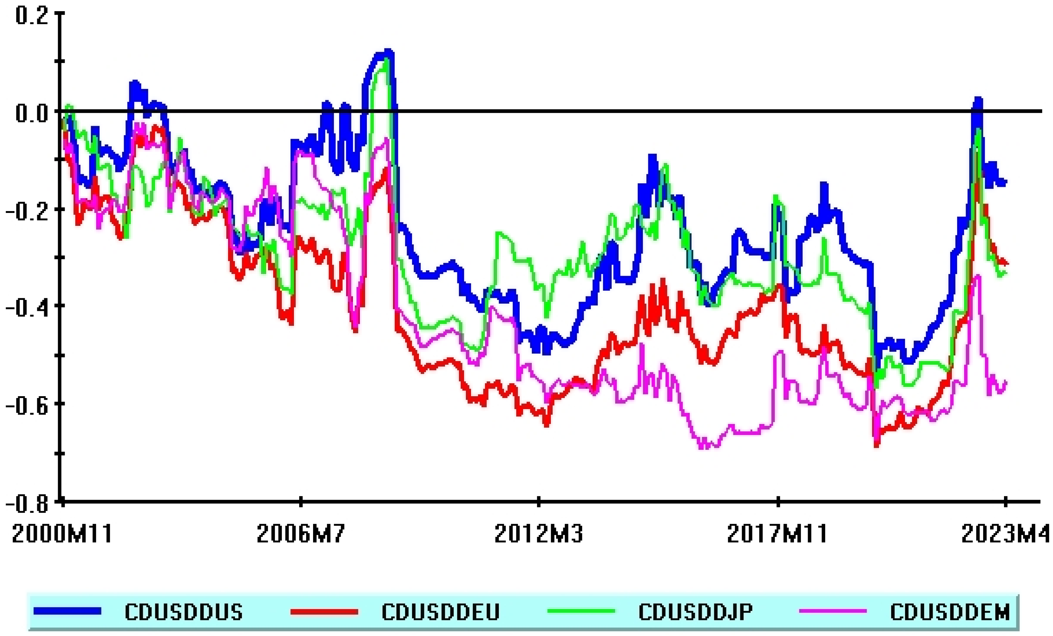
Figure 2.
Conditional correlations between US Dollar returns and stock returns. Actual values versus recursive forecasts. Monthly data: May 2001–April 2023.
Figure 2.
Conditional correlations between US Dollar returns and stock returns. Actual values versus recursive forecasts. Monthly data: May 2001–April 2023.

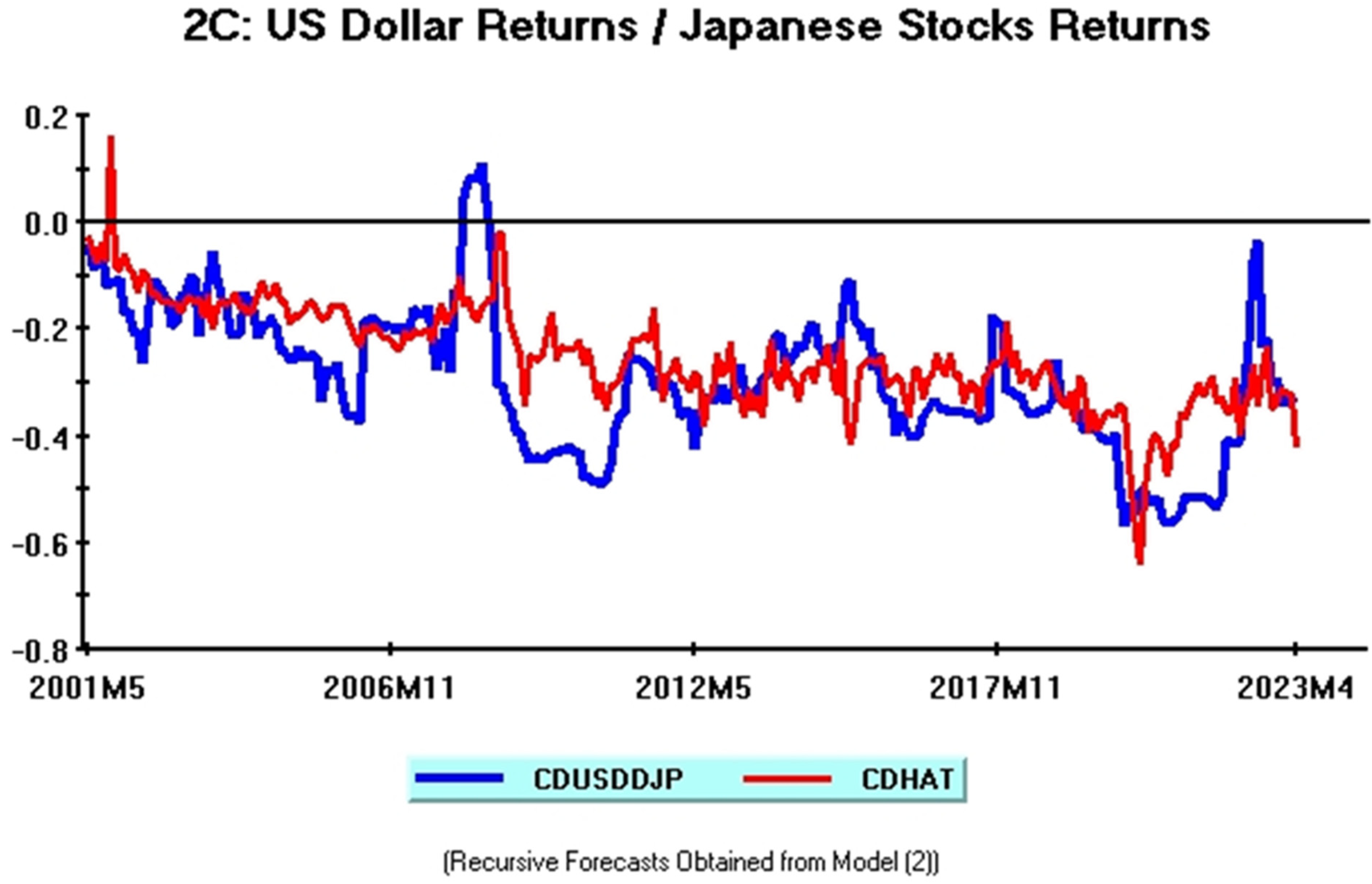
Figure 3.
Time-varying effects of lagged US Expected Inflation coefficients on conditional correlations: a comparison.
Figure 3.
Time-varying effects of lagged US Expected Inflation coefficients on conditional correlations: a comparison.
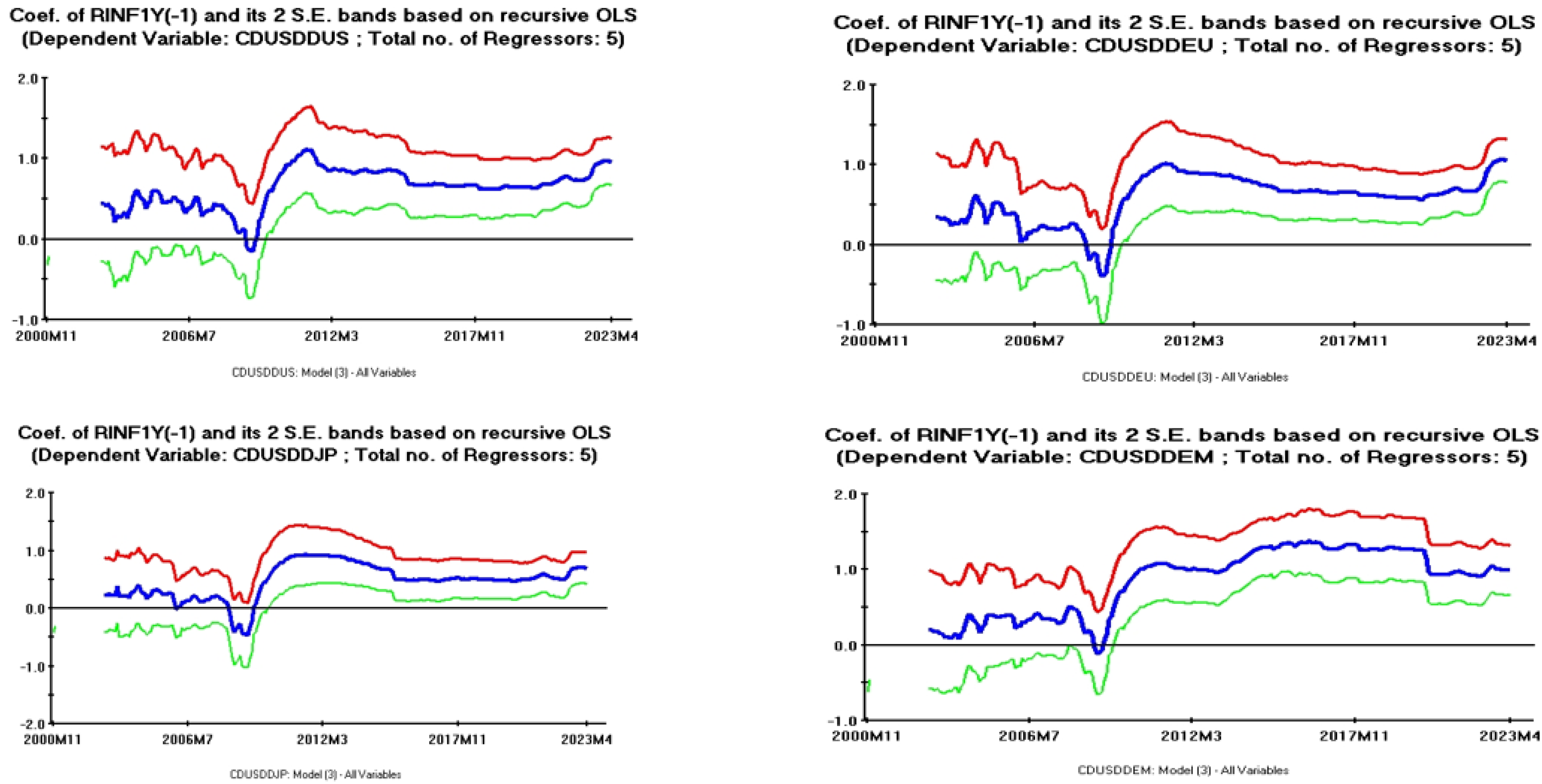
Figure 4.
Time-varying effects of lagged World Economic Policy Uncertainty coefficients on conditional correlations: a comparison.
Figure 4.
Time-varying effects of lagged World Economic Policy Uncertainty coefficients on conditional correlations: a comparison.
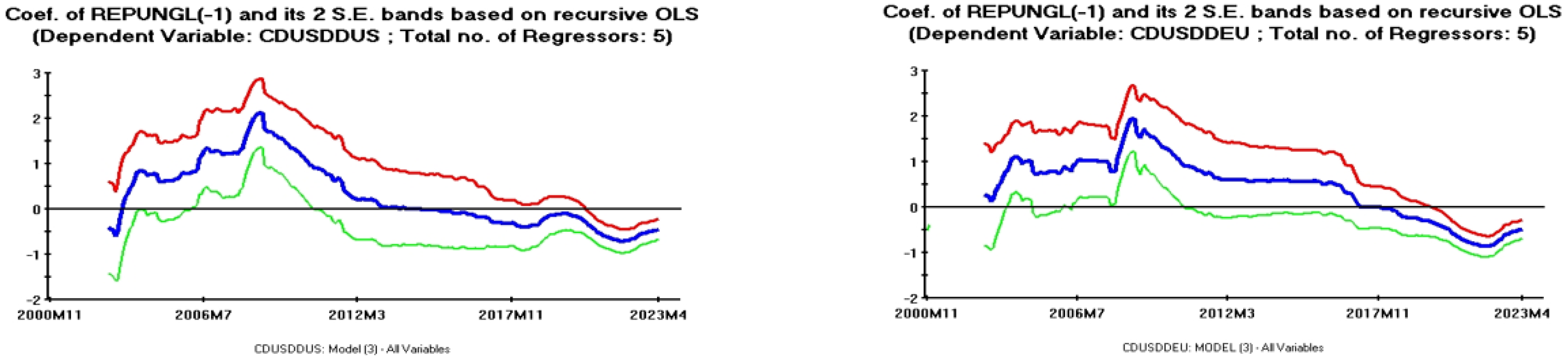
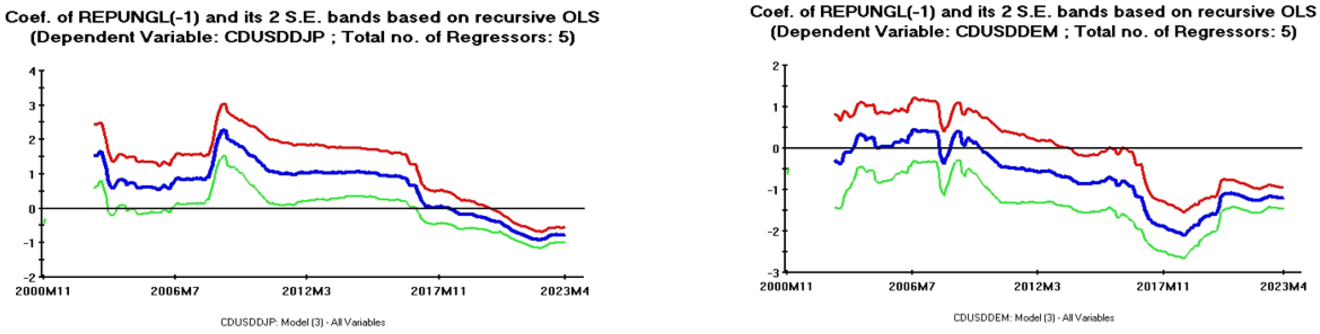
Figure 5.
Time-varying effects of lagged World Equity Risk Premium coefficients on conditional correlations: a comparison.
Figure 5.
Time-varying effects of lagged World Equity Risk Premium coefficients on conditional correlations: a comparison.


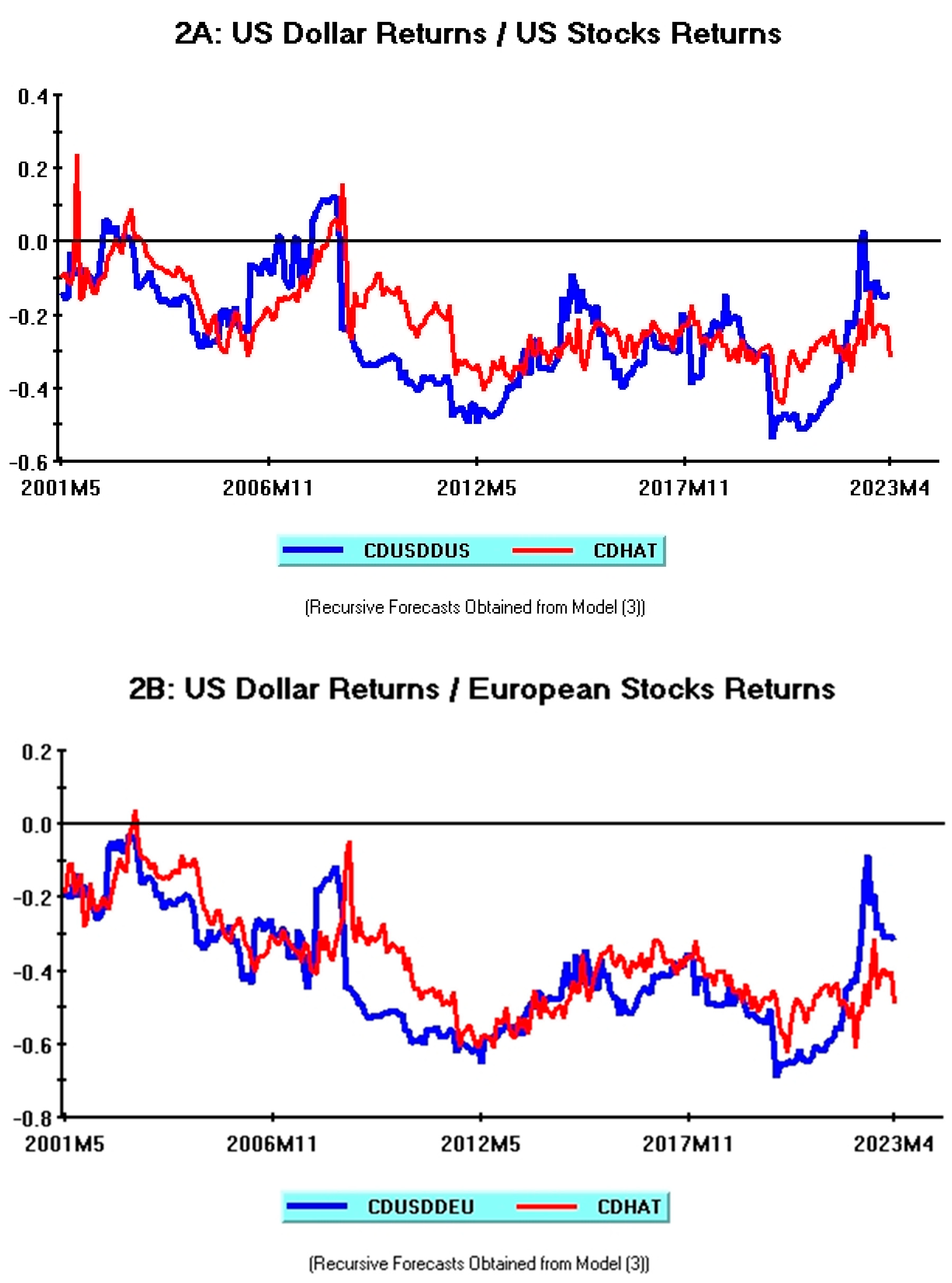
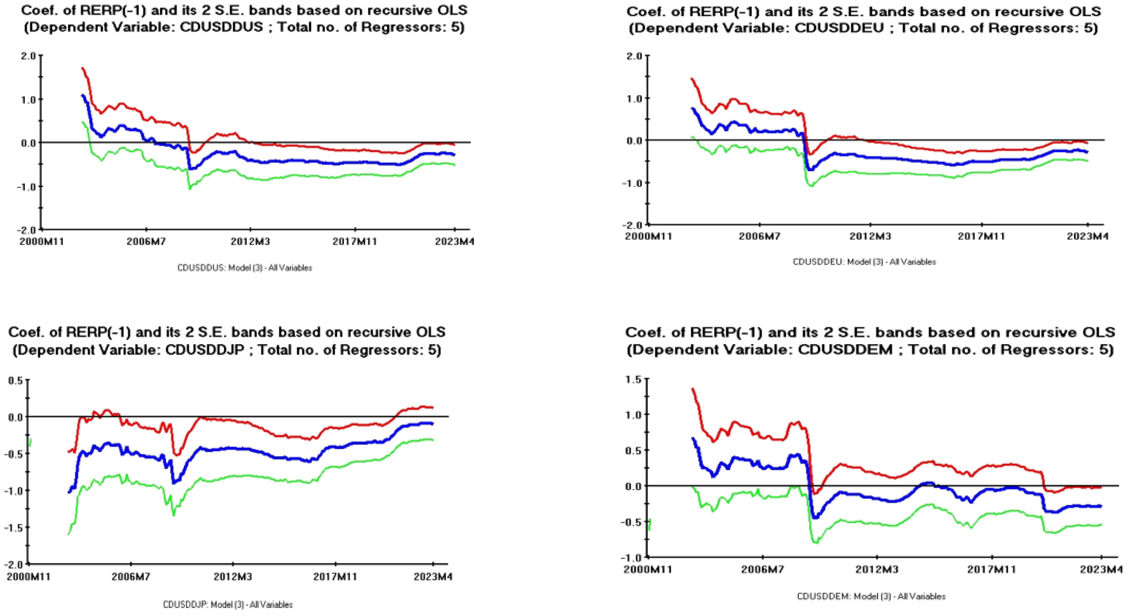
Table 1.
Effects of Single Macroeconomic and Financial Variables on Returns Correlations. Monthly Data: November 2000–April 2023 (270 Obs.).
Table 1.
Effects of Single Macroeconomic and Financial Variables on Returns Correlations. Monthly Data: November 2000–April 2023 (270 Obs.).
| Variables | USD/European Stocks | USD/US Stocks | USD/Em. Mark. Stocks | USD/Japanese Stocks | ||||
|---|---|---|---|---|---|---|---|---|
| α | R2 | α | R2 | α | R2 | α | R2 | |
| CBOE VIX | 0.060 | 0.001 | 0.07 | 0.001 | 0.06 | 0.011 | −0.08 | 0.002 |
| (0.21) | (0.28) | (0.72) | (−0.40) | |||||
| Equity Market Volatility Tracker | 0.07 | 0.041 | 0.07 | 0.038 | 0.06 | 0.017 | 0.05 | 0.023 |
| (1.01) | (1.30) | (0.72) | (0.90) | |||||
| ECB Systemic Stress | −0.09 | 0.008 | 0.002 | 0.000 | 0.02 | 0.000 | −0.03 | 0.001 |
| (−0.63) | (0.12) | (0.70) | (−0.25) | |||||
| World Equity Risk Premium | −1.00 *** | 0.465 | −0.83 *** | 0.349 | −1.18 *** | 0.422 | −0.57 *** | 0.212 |
| (−7.59) | (−6.01) | (−5.22) | (−4.04) | |||||
| US 1-Year Expected Inflat. | 1.32 *** | 0.288 | 1.25 *** | 0.291 | 1.40 *** | 0.215 | 0.88 *** | 0.184 |
| (5.81) | (5.12) | (3.27) | (3.41) | |||||
| World Economic Pol. Uncertainty | −0.88 ** | 0.166 | −0.78 ** | 0.145 | −1.57 *** | 0.350 | −0.93 *** | 0.262 |
| (−2.76) | (−2.52) | (−5.40) | (−4.03) | |||||
| Oil Price | −0.22 ** | 0.169 | −0.13 | 0.063 | −0.22 * | 0.101 | −0.04 | 0.009 |
| (−2.14) | (−1.23) | (−1.78) | (−0.50) | |||||
| US Term Structure | 0.04 | 0.001 | −0.08 | 0.003 | 0.19 | 0.012 | 0.11 | 0.009 |
| (0.16) | (−0.38) | (0.58) | (0.58) | |||||
| US Consumer Confidence | 1.08 | 0.027 | 0.93 | 0.022 | −0.67 | 0.006 | 0.04 | 0.000 |
| (1.02) | (0.94) | (−0.59) | (0.04) | |||||
Notes: Estimated equations have the following specification ⍴USD,j,t = c + αvt + εt, where ⍴USD,j,t: conditional correlation between the defensive asset (US Dollar) and stock price (j: European Stocks; US Stocks; Emerging Markets Stocks; Japanese Stocks) returns at time (t). c: constant term; vt: single macroeconomic or financial indicator at time (t); εt: error term. Newey and West (1987) heteroscedasticity and autocorrelation consistent estimates. t-statistics in parentheses below parameters estimates. ***: significant at a 1% level; **: significant at a 5% level; *: significant at a 10% level.
Table 2.
Multiple regressions: Effects of Selected Macroeconomic and Financial Variables on Returns Correlations. Monthly Data: November 2000–April 2023 (270 Obs.).
Table 2.
Multiple regressions: Effects of Selected Macroeconomic and Financial Variables on Returns Correlations. Monthly Data: November 2000–April 2023 (270 Obs.).
| Estimated Coefficients | USD/European Stocks | USD/US Stocks | USD/Em. Mark. Stocks | USD/Japanese Stocks | ||||
|---|---|---|---|---|---|---|---|---|
| c | −0.30 *** | (−3.47) | −0.19 ** | (−2.24) | −0.21 ** | (−2.43) | −0.26 *** | (−2.96) |
| β1 | −0.48 * | (−1.77) | −0.44 | (−1.57) | −1.18 *** | (−4.35) | −0.75 *** | (−3.53) |
| β2 | −0.29 * | (−1.67) | −0.29 | (−1.27) | −0.28 | (−1.04) | −0.10 | (−0.55) |
| β3 | −0.17 ** | (−2.34) | −0.07 | (−0.98) | −0.16 | (−1.56) | −0.01 | (−0.20) |
| β4 | 1.04 *** | (4.26) | 0.96 *** | (4.54) | 0.98 *** | (4.09) | 0.69 *** | (2.89) |
| Overall Regression Fit, Regression Standard Errors, F-Statistic | ||||||||
| R2 | 0.590 | 0.476 | 0.598 | 0.402 | ||||
| S.E. | 0.104 | 0.112 | 0.128 | 0.106 | ||||
| F-Stat. | 95.6 *** | 60.4 *** | 98.7 *** | 44.5 *** | ||||
Notes: Estimated equations have the following specification: ⍴USD, j, t = c + β1 (Repungl)t−1 + β2 (Rerp)t−1 + β3 (Roil)t−1 + β4 (Rinf1Y)t−1 + εt, where: ⍴USD,j,t: conditional correlation between the defensive asset (USD: US Dollar) and stock price (j: European Stocks; US Stocks; Emerging Markets Stocks; Japanese Stocks) returns at time (t); c: constant term; Repungl: World Economic Policy Uncertainty Index (rescaled by/1000); Rerp: World Equity Risk Premium (rescaled by/10); Roil: Oil Price (rescaled by/100); Rinf1Y: US 1-year Expected Inflation (rescaled by/10); εt: error term. Newey and West (1987) heteroscedasticity and autocorrelation consistent estimates. t-statistics in parentheses below parameters estimates. ***: significant at a 1% level; **: significant at a 5% level; *: significant at a 10% level.
Table 3.
Forecasting Performance of Alternative Models. Monthly Data: May 2001–April 2023 (264 observations).
Table 3.
Forecasting Performance of Alternative Models. Monthly Data: May 2001–April 2023 (264 observations).
| Models | CDUSDDEU | CDUSDDUS | CDUSDDEM | CDUSDDJP | ||||
|---|---|---|---|---|---|---|---|---|
| MODEL 1 (Rinf1y)t−1 | MAE: | 0.115 | MAE: | 0.107 | MAE: | 0.132 | MAE: | 0.099 |
| RMSE: | 0.139 | RMSE: | 0.130 | RMSE: | 0.179 | RMSE: | 0.124 | |
| PT TEST: | n.a. | PT TEST: | 2.097 ** | PT TEST: | n.a. | PT TEST: | n.a. | |
| MODEL 2 (Rinf1y)t−1; (Repungl)t−1 | MAE: | 0.099 | MAE: | 0.101 | MAE: | 0.120 | MAE: | 0.085 |
| RMSE: | 0.129 | RMSE: | 0.122 | RMSE: | 0.146 | RMSE: | 0.110 | |
| PT TEST: | n.a. | PT TEST: | −0.536 | PT TEST: | n.a. | PT TEST: | −0.152 | |
| MODEL 3 (All Variables)t−1 | MAE: | 0.087 | MAE: | 0.097 | MAE: | 0.107 | MAE: | 0.087 |
| RMSE: | 0.111 | RMSE: | 0.118 | RMSE: | 0.133 | RMSE: | 0.112 | |
| PT TEST: | n.a. | PT TEST: | 6.322 *** | PT TEST: | n.a. | PT TEST: | −0.153 | |
Notes: CDUSDDEU: Conditional Correlation US Dollar/European Stocks returns; CDUSDDUS: Conditional Correlation US Dollar/US Stocks returns; CDUSDDEM: Conditional Correlation US Dollar/Emerging Markets Stocks returns; CDUSDDJP: Conditional Correlation US Dollar/Japanese Stocks returns. Model 1: Estimated Equation: ⍴USD,j,t = c + β4 (Rinf1Y)t−1 + εt (Lagged US inflationary expectations only). Model 2: Estimated Equation: ⍴USD,j,t = c + β1 (Repungl)t−1 + β4 (Rinf1Y)t−1 + εt (Lagged US inflationary expectations; Lagged World Economic Policy Uncertainty). Model 3: Estimated Equation: ⍴USD,j,t = c + β1 (Repungl)t−1 + β2 (Rerp)t−1 + β3 (Roil)t−1 + β4 (Rinf1Y)t−1 + εt (All Lagged Variables). See notes in Table 2 for the meaning of all symbols appearing in estimated equations.
Disclaimer/Publisher’s Note: The statements, opinions and data contained in all publications are solely those of the individual author(s) and contributor(s) and not of MDPI and/or the editor(s). MDPI and/or the editor(s) disclaim responsibility for any injury to people or property resulting from any ideas, methods, instructions or products referred to in the content. |
© 2024 by the author. Licensee MDPI, Basel, Switzerland. This article is an open access article distributed under the terms and conditions of the Creative Commons Attribution (CC BY) license (https://creativecommons.org/licenses/by/4.0/).
Share and Cite
MDPI and ACS Style
Tronzano, M. What Drives Asset Returns Comovements? Some Empirical Evidence from US Dollar and Global Stock Returns (2000–2023). J. Risk Financial Manag. 2024, 17, 167. https://doi.org/10.3390/jrfm17040167
AMA Style
Tronzano M. What Drives Asset Returns Comovements? Some Empirical Evidence from US Dollar and Global Stock Returns (2000–2023). Journal of Risk and Financial Management. 2024; 17(4):167. https://doi.org/10.3390/jrfm17040167
Chicago/Turabian StyleTronzano, Marco. 2024. "What Drives Asset Returns Comovements? Some Empirical Evidence from US Dollar and Global Stock Returns (2000–2023)" Journal of Risk and Financial Management 17, no. 4: 167. https://doi.org/10.3390/jrfm17040167